Optimal vaccination program for two infectious diseases with cross immunity
Abstract
There are often multiple diseases with cross immunity competing for vaccination resources. Here we investigate the optimal vaccination program in a two-layer Susceptible-Infected-Removed (SIR) model, where two diseases with cross immunity spread in the same population, and vaccines for both diseases are available. We identify three scenarios of the optimal vaccination program, which prevents the outbreaks of both diseases at the minimum cost. We analytically derive a criterion to specify the optimal program based on the costs for different vaccines.
Vaccination is an effective method of preventing epidemics like COVID-19, diphtheria, influenza, and measles Andre et al. (2008); Bonanni (1999); Le et al. (2020). Mathematical models have been commonly used to examine the effect of vaccination on epidemic control and prevention Wang et al. (2016); Dykman et al. (2008); Khanjanianpak et al. (2020). Vaccines help the human body’s natural defense systems to develop antibodies to pathogens. Generally, antibodies to one pathogen do not provide protection to another pathogen. However, there is increasing evidence of cross immunity between diseases, where exposure to one pathogen may help protect against other pathogens. Wu et al. (2020); Schultz-Cherry (2015); Balmer and Tanner (2011); Laurie et al. (2015, 2018). Cross immunity is a common outcome when some diseases caused by related pathogens spread in the same population. There is rich previous epidemiological research on the interactions pathogens with cross immunity from the perspectives of age, gender, and population structure Andreasen et al. (1997); Castillo-Chavez et al. (1989, 1996); Li et al. (2003); Webb et al. (2013); Leventhal et al. (2015); Darabi Sahneh and Scoglio (2014); Azimi-Tafreshi (2016). Some physical literature provides analytic calculations of the expected final epidemic sizes of multiple diseases coexisting in the same population Karrer and Newman (2011); Newman (2005). It is needed to take into account the effect of cross immunity while developing disease prevention strategies. Some studies gave simulation and optimization frameworks to identify the effective resource allocation to control several competitive diseases in the susceptible-infected-susceptible (SIS) model Watkins et al. (2016); Chen and Preciado (2014). However, the identification of the optimal vaccination programs to control competitive diseases with cross immunity in the susceptible-infected-recovered (SIR) model is under-researched and critically-needed, particularly when the world is expecting to face the challenge of allocating COVID-19 vaccines in the coming years.
In this letter, we assume that there are two vaccines for two SIR type diseases with varying cost. A vaccination program specifies the fractions of individuals that should be vaccinated for each vaccine. We define that the optimal vaccination program can control the outbreak of both diseases at the minimum cost. The microscopic Markov chain approach (MMCA) is adopted to derive the conditions guaranteeing that both diseases can be contained in the population. An optimization framework is proposed to analytically derive the optimal vaccination program. We identify three scenarios of the optimal vaccination program, and derive a criterion to specify the optimal program based on the costs for different vaccines.
Here, we consider a two-layer network with the same topological structure, which represents the transmission channels for both diseases, , which propagate through different layers. Nodes represent individuals, which are susceptible (), infected (), or recovered () for disease . A susceptible node can be infected by an infected node with an infection rate . An infected node has a transition rate to become recovered and immune to disease . The susceptibility to disease () of individuals recovered from disease is reduced by a factor (i.e., the actual infection rate for disease becomes ). quantifies the level of cross immunity. In the extreme case, corresponds to complete cross immunity, and corresponds to a simpler problem without cross immunity. An individual can be simultaneously infected by both diseases. Before the occurrence of the first node infected with disease , a fraction of nodes are provided with vaccines for disease . We assume that vaccine-induced immunity is equivalent to the natural immunity obtained from actual infection. Thus, vaccines for disease directly transfer the node state from to without causing illness. Nodes vaccinated with vaccines for disease are also immune to disease and have a susceptibility to disease () reduced by a factor . After vaccination, a small fraction of unvaccinated nodes become initially infected for both diseases.
According to this scheme, every node can be in nine different states at each time: , , , , , , , , and . Note that the character order does not affect the state (e.g., is equivalent to ). Every node has a certain probability of being in one of the nine states at time denoted by , , , , , , , , and . . For disease at time , node has a certain probability of being in one of three states , , or , denoted by
| (1) | ||||
where . due to the effect of vaccination. If node is recovered from disease , the probability of not being infected for disease () is
| (2) |
where is the adjacency matrix on both layers. If node is not recovered from disease , the probability is
| (3) |
We develop the microscopic Markov chain approach to analyze the state transitions for each node as
| (4) |
The fractions of susceptible, infected, and recovered nodes at time for disease is denoted by , , and , respectively.
| (5) | |||
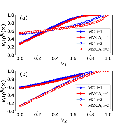
Here is the number of nodes on the network. The fraction of uninfected nodes at the stationary state (when ) is for disease . We perform extensive Monte Carlo simulations (MC) to validate the MMCA results obtained by Eqs. (4). We adopt the synchronous updating method in MC simulations. All nodes update their states simultaneously in each time step, which is set as 1. We consider a network of 2000 nodes with a Poisson degree distribution, where the mean degree is 20. The initial fraction of infected nodes is for diseases if . Each point in Fig. 1 is obtained by averaging 1000 MC simulations. The average is 0.96, indicating a high agreement between MMCA and MC simulation results.
Next, we explore the conditions preventing the outbreaks of both diseases. Specifically, the outbreak of disease can be prevented when
| (6) |
| (7) |
According to Eq. (1) and Eq. (4),
| (8) |
Thus,
| (9) |
If , , , and . Thus, , , and . If is large enough, , consequently, from Eq. (2) and Eq. (3), we obtain
| (10) |
where is the degree of node . Thus,
| (11) |
where is the mean degree of the network. To ensure the failure of outbreaks for both diseases, the right-hand side of Eq. (11) should be less or equal to 0, because it is slightly larger than the left-hand side. Therefore, the following conditions should be met
| (12) | ||||
where and . and are the basic reproduction numbers for disease 1 and disease 2, respectively. If , , disease can never spread out and Eqs. (12) still hold. Here is the expected number of infections caused by an individual infected with disease when the fractions of vaccinated individuals are and at the beginning. Note that this corresponds to for . According to Eqs. (12), in order to prevent the outbreaks of both diseases, the following conditions should be met
| (13) | ||||
From Eqs. (13), we observe that fewer vaccines for disease are needed to prevent the outbreak of disease if more nodes are vaccinated for disease (). When (all nodes are vaccinated for disease ), , indicating that the minimum fraction of nodes that should be vaccinated for disease to prevent the outbreak of disease is . We define this value as
| (14) |
In the following, we consider the common scenario when and . The results can be easily extended to other scenarios.
Now we plot the full phase diagram of the outbreak conditions for both diseases in Fig. 2. We adopt the same two-layer network setting as Fig. 1. As illustrated in Fig. 2, only points of () in region II can prevent the outbreaks of both diseases. The intersection satisfies that
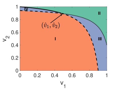
| (15) | ||||
Denote ,
| (16) |
Next, we aim to identify the minimum vaccination cost that can prevent the outbreaks of both diseases. Denote and as the costs of vaccination per capita for disease 1 and disease 2, respectively. and are positive. The total vaccination cost is . Then, we formulate the following optimization problem
| minimize | (17) | |||||
| subject to | ||||||
Since the slopes for and are both positive, the optimal vaccination program (, ) is on the boundary of region II in Fig. 2.
On the solid line (the boundary between region II and region IV),
and , thus,
| (18) |
| (19) |
Therefore, is a concave function of . The optimal vaccination program (, ) is either or . Similarly, on the dotted line (the boundary between region II and region III), the optimal vaccination program (, ) is either or . Overall, there are three potential scenarios of the optimal vaccination program: (1, ), (, 1), and ().
Comparing the values of on these points, we find that the value of is determined by the following four nonnegative parameters:
| (20) | ||||||
| (21) |
If , we have
thus,
| (22) |
If , we have
thus,
| (23) |
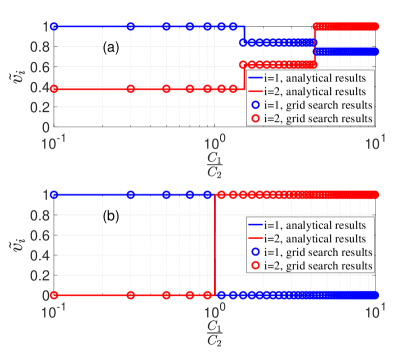
According to the criterion above, we can analytically derive the optimal vaccination program by substituting and to Eq. (22) and Eq. (23). In Fig. 3, the optimal vaccination programs derived by analytical results are compared with the grid search with respect to different vaccine cost ratios for different diseases. The agreement is high. In Fig. 3(a), , , , , so . As a result, there are three scenarios according to the vaccine cost ratio. In Fig. 3(b), , , , , so . As a result, there are two scenarios according to the vaccine cost ratio.
In summary, we investigate the optimal vaccination program that can prevent the outbreaks of two SIR type diseases with cross immunity at the minimum cost. We adopt MMCA to develop an optimization framework to identify the optimal vaccination programs in various epidemiological parameter settings. We analytically derive the optimal solutions and validate the results with MC simulations and grid search. This study provides clues to design effective and efficient vaccination programs where the cross immunity between multiple diseases exists. In particular, the world is facing critical challenges in confronting the coexistence of both the novel coronavirus (COVID-19) pandemic and other major infectious diseases Mateus et al. (2020). With limited resources, it is important to inform the model-driven vaccination programs that can contain multiple epidemics efficiently.
References
- Andre et al. (2008) F. E. Andre, R. Booy, H. L. Bock, J. Clemens, S. K. Datta, T. J. John, B. W. Lee, S. Lolekha, H. Peltola, T. Ruff, et al., Bulletin of the World health organization 86, 140 (2008).
- Bonanni (1999) P. Bonanni, Vaccine 17, S120 (1999).
- Le et al. (2020) T. T. Le, Z. Andreadakis, A. Kumar, R. G. Roman, S. Tollefsen, M. Saville, and S. Mayhew, Nat Rev Drug Discov 19, 305 (2020).
- Wang et al. (2016) Z. Wang, C. T. Bauch, S. Bhattacharyya, A. d’Onofrio, P. Manfredi, M. Perc, N. Perra, M. Salathé, and D. Zhao, Physics Reports 664, 1 (2016).
- Dykman et al. (2008) M. I. Dykman, I. B. Schwartz, and A. S. Landsman, Phys. Rev. Lett. 101, 078101 (2008).
- Khanjanianpak et al. (2020) M. Khanjanianpak, N. Azimi-Tafreshi, and C. Castellano, Phys. Rev. E 101, 062306 (2020).
- Wu et al. (2020) A. Wu, V. T. Mihaylova, M. L. Landry, and E. F. Foxman, The Lancet Microbe 1, e254 (2020).
- Schultz-Cherry (2015) S. Schultz-Cherry, “Viral interference: the case of influenza viruses,” (2015).
- Balmer and Tanner (2011) O. Balmer and M. Tanner, The Lancet Infectious Diseases 11, 868 (2011).
- Laurie et al. (2015) K. L. Laurie, T. A. Guarnaccia, L. A. Carolan, A. W. Yan, M. Aban, S. Petrie, P. Cao, J. M. Heffernan, J. McVernon, J. Mosse, et al., The Journal of infectious diseases 212, 1701 (2015).
- Laurie et al. (2018) K. L. Laurie, W. Horman, L. A. Carolan, K. F. Chan, D. Layton, A. Bean, D. Vijaykrishna, P. C. Reading, J. M. McCaw, and I. G. Barr, The Journal of infectious diseases 217, 548 (2018).
- Andreasen et al. (1997) V. Andreasen, J. Lin, and S. A. Levin, Journal of mathematical biology 35, 825 (1997).
- Castillo-Chavez et al. (1989) C. Castillo-Chavez, H. W. Hethcote, V. Andreasen, S. A. Levin, and W. M. Liu, Journal of mathematical biology 27, 233 (1989).
- Castillo-Chavez et al. (1996) C. Castillo-Chavez, W. Huang, and J. Li, SIAM Journal on Applied Mathematics 56, 494 (1996).
- Li et al. (2003) J. Li, Z. Ma, S. P. Blythe, and C. Castillo-Chavez, Journal of mathematical biology 47, 547 (2003).
- Webb et al. (2013) S. D. Webb, M. J. Keeling, and M. Boots, Journal of theoretical biology 324, 21 (2013).
- Leventhal et al. (2015) G. E. Leventhal, A. L. Hill, M. A. Nowak, and S. Bonhoeffer, Nature communications 6, 6101 (2015).
- Darabi Sahneh and Scoglio (2014) F. Darabi Sahneh and C. Scoglio, Phys. Rev. E 89, 062817 (2014).
- Azimi-Tafreshi (2016) N. Azimi-Tafreshi, Phys. Rev. E 93, 042303 (2016).
- Karrer and Newman (2011) B. Karrer and M. E. J. Newman, Phys. Rev. E 84, 036106 (2011).
- Newman (2005) M. E. J. Newman, Phys. Rev. Lett. 95, 108701 (2005).
- Watkins et al. (2016) N. J. Watkins, C. Nowzari, V. M. Preciado, and G. J. Pappas, IEEE Transactions on Control of Network Systems 5, 298 (2016).
- Chen and Preciado (2014) X. Chen and V. M. Preciado, in 53rd IEEE Conference on Decision and Control (2014) pp. 6209–6214.
- Mateus et al. (2020) J. Mateus, A. Grifoni, A. Tarke, J. Sidney, S. I. Ramirez, J. M. Dan, Z. C. Burger, S. A. Rawlings, D. M. Smith, E. Phillips, et al., Science 370, 89 (2020).