Optimal Sensor and Actuator Selection for Factored Markov Decision Processes: Complexity, Approximability and Algorithms
Abstract
Factored Markov Decision Processes (fMDPs) are a class of Markov Decision Processes (MDPs) in which the states (and actions) can be factored into a set of state (and action) variables. The state space, action space and reward function of a fMDP can be encoded compactly using a factored representation. In this paper, we consider the setting where we have a set of potential sensors to select for the fMDP (at design-time), where each sensor measures a certain state variable and has a selection cost. We formulate the problem of selecting an optimal set of sensors for fMDPs (subject to certain budget constraints) to maximize the expected infinite-horizon discounted return provided by the optimal control policy. We show the fundamental result that it is NP-hard to approximate this optimization problem to within any non-trivial factor. We then study the dual problem of budgeted actuator selection (at design-time) to maximize the expected return under the optimal policy. Again, we show that it is NP-hard to approximate this optimization problem to within any non-trivial factor. Furthermore, with explicit examples, we show the failure of greedy algorithms for both the sensor and actuator selection problems and provide insights into the factors that cause these problems to be challenging. Despite the inapproximability results, through extensive simulations, we show that the greedy algorithm may provide near-optimal performance for actuator and sensor selection in many real-world and randomly generated fMDP instances.111This material is based upon work supported by the Office of Naval Research (ONR) via Contract No. N00014-23-C-1016 and under subcontract to Saab, Inc. as part of the TSUNOMI project. Any opinions, findings and conclusions or recommendations expressed in this material are those of the author(s) and do not necessarily reflect the views of ONR, the U.S. Government, or Saab, Inc.
The authors are with the Elmore Family School of Electrical and Computer Engineering, Purdue University, West Lafayette IN 47907 USA. Email addresses: {jbhargav, mahsa, sundara2}@purdue.edu
Keywords: Computational complexity, Greedy algorithms, Markov Decision Processes, Optimization, State estimation, Sensor and Actuator selection.
1 Introduction
Markov Decision Processes (MDPs) have been widely used to model systems in decision-making problems such as autonomous driving, multi-agent robotic task execution, large data center operation and machine maintenance [1, 2]. In the MDP framework, the states of the system evolve stochastically owing to a probabilistic state transition function. In many real-world sequential decision-making problems, the state space is quite large (growing exponentially with the number of state variables). However, many large MDPs often admit significant internal structure, which can be exploited to model and represent them compactly. The idea of compactly representing a large structured MDP using a factored model was first proposed in [3]. In this framework, the state of a large MDP is factored into a set of state variables, each taking values from their respective domains. Then, a dynamic Bayesian network (DBN) can be used to represent the transition model. Assuming that the transition of a state variable only depends on a small subset of all the state variables, a DBN can capture this dependence in a very compact manner. Furthermore, the reward function can also be factored into a sum of rewards related to individual variables or a small subset of variables.
Factored MDPs exploit both additive and context-specific structures in large scale systems. However, a factored representation may still result in the intractability of exactly solving such large fMDPs. A significant amount of work has focused on solving for the optimal policy in fMDPs [4, 5] and its variants like Partially Observable MDPs (POMDPs) [6, 7] and Mixed-Observable MDPs (MOMDPs) [8]. However, these algorithms primarily focus on reducing the computational time required for solving large state space MDPs and its variants, but do not study the problem of sensor and actuator set selection for such systems in order to achieve optimal performance. While the problem of sensor and actuator selection has been well studied for other classes of systems (e.g., linear systems) [9, 10, 11], there has been no prior work on optimal sensor/actuator selection for fMDPs.
1.1 Motivation
Many applications in large-scale networks like congestion control [12, 13], load-balancing [14, 15] and energy optimization in large data-centers [1, 2] suffer from limited sensing and actuating resources. In many autonomous systems, the number of sensors or actuators that can be installed is limited by a certain budget and system design constraints [16]. In robotics applications, system designers often face the challenge of achieving certain design objectives such as maximizing observability and performance of the robot [16] [17][18], under limited sensing or actuating resources.
Scenario 1: Consider a task where a team of mobile robots have to simultaneously localize themselves (i.e., estimate their state) and perform tasks in an environment (see Figure 1). The robots can communicate with sensors deployed in the environment to localize themselves. Each robot has an underlying MDP and receives rewards for successfully completing tasks. Due to limited budget, a central designer can only deploy a limited number of sensors in the environment. The designer has to select an optimal subset of sensors to be placed in order to localize (i.e., estimate the states of) the robots, which can maximize the overall reward obtained by the team of robots.

Scenario 2: Consider a complex electric distribution network consisting of interconnected micro-grid systems, each containing generation stations, substations, transmission lines and electric loads, as shown in Figure 2. Each node in the network is prone to electric faults (e.g., generator faults, short circuit faults in the load). Faults in a node can potentially cascade, and cause a catastrophic power blackout in the entire network. Due to limited budget, a grid safety designer has to select only a subset of nodes where sensors and actuators can be installed, which can help minimize fault percolation in the network, by identifying and isolating (known as islanding) certain critical nodes.
The multi-agent systems described above can be modelled as MDPs, and often have exponentially large state and action spaces in practice (e.g., a large number of nodes in the network). In such cases, one can leverage the internal structure of such systems and model them as fMDPs. If one can only measure a subset of state variables using a limited number of sensors or can only influence transitions of a subset of state variables using a limited number of actuators, one is faced with the problem of selecting the optimal set of sensors (or actuators) that can result in better performance of such systems (fMDPs), which has not been well studied in the literature.
In this paper, we focus on two problems related to fMDPs: (i) selecting the best set of sensors at design-time (under some budget constraints) for a fMDP which can maximize the optimal expected infinite-horizon return for the resulting optimal policy and (ii) selecting the best set of actuators at design-time (under some budget constraints) for a fMDP which can maximize the optimal expected infinite-horizon return provided by the optimal policy.

1.2 Related Work
Sequential sensor placement/selection has been studied in the context of MDPs and its variants like POMDPs. In [20], the authors consider active perception under a limited budget for POMDPs to selectively gather information at runtime. However, in our problem, we consider design-time sensor/actuator selection for fMDPs, where the sensor/actuator set is not allowed to dynamically change at runtime. A body of literature considers the problem of sensor scheduling for sequential decision-making tasks and model the task of sensor placement itself as a POMDP [21, 22]. However, we consider the problem of selecting the optimal set of sensors (or actuators) a priori (at design-time) for an fMDP, and not sequentially.
The problem of selecting an optimal subset of sensors has also been very well studied for linear systems. In [9] and [10], the authors study the sensor selection and sensor attack problems for Kalman filtering of linear dynamical systems, where the objective is to reduce the trace of the steady-state error covariance of the filter. The authors of [10] show that these problems are NP-Hard and there exists no polynomial-time constant-factor approximation algorithms for such class of problems. In [23], the authors propose balanced model reduction and greedy optimization technique to efficiently determine sensor and actuator selections that optimize observability and controllability for linear systems. In [24], the authors show that the mapping from subsets of possible actuator/sensor placements to any linear function of the associated controllability or observability Gramian is a modular set function. This strong property of the function allows efficient global optimization.
Many works have considered the problem of actuator selection for controlling and stabilizing large scale power grids. The authors of [25] consider the problem of optimal placement of High Voltage Direct Current (HVDC) links in a power system. HVDC links are actuators which are used to stabilize a power grid from oscillations. They propose a performance measure that can be used to rank different candidate actuators according to their behavior after a disturbance, which is computed using Linear Matrix Inequalities (LMIs). In [26], the authors propose an algorithm using Semi-Definite Programming (SDP) for placement of HVDC links, which can optimize the LMI-based performance measure proposed in [25]. The authors of [26] state that this technique can be applied to other actuator selection problems, such as Flexible AC Transmission (FACTS) controllers and Power System Stabilizers (PSS). However, these techniques use a linearized state-space model of the power system around the current operating point, whereas in this paper, we consider fMDP models which may not necessarily have a linear structure.
For combinatorially-hard sensor or actuator selection problems, various approximation algorithms have proven to produce near-optimal solutions [27][28]. In [29], the authors leverage the adaptive submodularity property of the sensor area coverage metric to learn an adaptive greedy policy for sequential sensor placement with provable performance guarantees. However, we consider the design-time sensor selection problem for fMDPs. The authors of [30] exploit the weak-submodularity property of the objective function and provide near-optimal greedy algorithms for sensor selection. In contrast to these results, we present worst-case in-approximability results and demonstrate how greedy algorithms for both sensor and actuator selection in fMDPs can perform arbitrarily poorly, and that the value function of a fMDP is not generally submodular in the set of sensors (or actuators) selected.
1.3 Contributions
Our contributions are as follows. Firstly, we show that the problem of selecting an optimal subset of sensors at design-time for a general class of factored MDPs is NP-hard, and there is no polynomial time algorithm that can approximate this problem to within a factor of of the optimal solution, for any , even when one has access to an oracle that can compute the optimal policy for any given instance (which itself is known to be PSPACE-hard [31]). Second, we show that the same inapproximability results hold for the problem of selecting an optimal subset of actuators at design-time for a general class of factored MDPs. Our inapproximability results directly imply that greedy algorithms cannot provide constant-factor guarantees for our problems, and that the value function of the fMDP is not submodular (in general) in the set of sensors (resp. actuators) selected. Our third contribution is to explicitly show how greedy algorithms can provide arbitrarily poor performance for fMDP-SS (resp. fMDP-AS) problems. Finally, through empirical results, we show that the greedy algorithm may provide near-optimal solutions for many instances in practice, despite the inapproximability results.
We considered the problem of optimal sensor selection for Mixed-Observable MDPs (MOMDPs) in the conference paper [32]. We proved its NP-hardness and provided insights into the lack of submodularity of the value function. However, in this paper, we present stronger inapproximability results for both sensor and actuator selection for a general class of factored MDPs, of which MOMDPs are a special case.
2 Problem Formulation
In this section, we formally state the sensor and actuator selection problems we consider in this paper. A general factored MDP is defined by the following tuple: , where is the state space decomposed into finite sub-spaces , each corresponding to a state-variable (which takes values from ), is the action space decomposed into finite sub-spaces , each corresponding to an action (which takes values from ), is the probabilistic state transition model, is the reward function and is the discount factor. The state transition model is usually represented using a DBN, which consists of a directed acyclic transition graph , that captures the relationship between state transitions of the variables . The reward function , is a scalar function of the factored state variables and actions . In many applications, the overall reward function is the sum of local rewards which depend on the local state-action pair .
2.1 The Sensor Selection Problem
Consider the scenario where there are no sensors installed initially, and the agent does not have observability of the state variables of the f-MDP. Instead, the agent has to select a subset of sensors to install. Define to be a collection of sensors, where the sensor measures exactly the state variable . Let be the cost we pay to measure state by placing the sensor , and let denote the total budget for the sensor placement. Let be the subset of sensors selected (at design-time) that generates observations . At time , the agent has the following information: observations , joint actions and rewards . Since the agent does not have complete observability, it maintains a belief over the states of the fMDP, , where is the belief space, which is the set of probability distributions over the states in .
In this case, the expected reward is belief-based, denoted as , and is given by , where is the belief over the state , is the action and is the reward obtained for taking action in the state . For any given choice of sensors, the agent seeks to maximize the expected infinite-horizon reward, given the initial belief , by finding an optimal policy satisfying with , where is the reward obtained at time . The policy belongs to a class of policies which map the history of observations, actions, and rewards to the next action. The value function under the policy can be computed using the value iteration algorithm with , and (as in [8]).
Let denote the set containing all the information the agent has until time . Define to be a class of history-dependent policies that map from a set containing all the information known to the agent until time to the action which the agent takes at time . The goal is to find an optimal subset of sensors , under the budget constraint, that can maximize the expected value of the infinite-horizon discounted return obtained by the agent under the optimal policy for the resulting POMDP. Specifically, we aim to solve the optimization problem:
We now define the decision version for the above optimization problem as the Factored Markov Decision Process Sensor Selection Problem (fMDP-SS Problem).
Problem 1 (fMDP-SS Problem).
Consider a fMDP and a set of sensors , where each sensor is associated with a cost . For a value and sensor budget , is there a subset of sensors , such that the expected return for the optimal policy in satisfies and the total cost of the sensors satisfies ?
2.2 The Actuator Selection Problem
Consider the scenario where there are no actuators installed initially, and the agent cannot influence the transitions of state variables of the fMDP. However, the agent has complete observability of the state variables . In this case, the agent has to select a subset of actuators to install. Define to be a collection of actuators, where the actuator provides a set of actions , and action can influence the state transition of . Let be the cost we pay to install the actuator , and let denote the total budget for the actuator placement. Let be the subset of actuators selected (at design-time).
Let denote the joint action space available to the agent generated by selecting the actuator set . If an actuator is not selected, then the agent has a default action , and by taking this action, the agent stays in its current state with probability 1. As the agent has complete observability of the state, the rewards depend on the joint state-action pairs, i.e., is the reward obtained by the agent for taking the joint action in state . Define to be a class of history-dependent policies that map from a set containing all the information known to the agent until time to action, which the agent takes at time .
The goal of the agent is to choose the best actuator set which can maximize the expected infinite-horizon discounted return under the optimal policy of the resulting MDP. The expected infinite-horizon discounted return is computed for the optimal policy satisfying with , where is the reward obtained at time . Let denote the expected infinite-horizon discounted return under the optimal policy for the actuator set . We aim to solve the optimization problem:
We now define the decision version of the above optimization problem as the Factored Markov Decision Process Actuator Selection Problem (fMDP-AS Problem).
Problem 2 (fMDP-AS Problem).
Consider a fMDP and a set of actuators , where each actuator is associated with a cost . For a value and actuator budget , is there a subset of actuators , such that the expected return for the optimal policy in satisfies and the total cost of the actuators selected satisfies ?
3 Complexity and Approximability Analysis
In this section, we analyze the approximability of the fMDP-SS and fMDP-AS problems. We will start with a brief overview of some relevant concepts from the field of computational complexity, and then provide some preliminary lemmas that we will use in proving our results. That will lead to our characterizations of the complexity of fMDP-SS and fMDP-AS.
3.1 Review of Complexity Theory
We first review the following fundamental concepts from complexity theory [33].
Definition 1.
A polynomial-time algorithm for a problem is an algorithm that returns a solution to the problem in a polynomial (in the size of the problem) number of computations.
Definition 2.
A decision problem is a problem whose answer is “yes” or “no”. The set P contains those decision problems that can be solved by a polynomial-time algorithm. The set NP contains those decision problems whose “yes” answer can be verified using a polynomial-time algorithm.
Definition 3.
An optimization problem is a problem whose objective is to maximize or minimize a certain quantity, possibly subject to constraints.
Definition 4.
A problem is NP-complete if (a) and (b) for any problem in NP, there exists a polynomial time algorithm that converts (or “reduces”) any instance of to an instance of such that the answer to the constructed instance of provides the answer to the instance of . is NP-hard if it satisfies (b), but not necessarily (a).
The above definition indicates that if one had a polynomial time algorithm for an NP-complete (or NP-hard) problem, then one could solve every problem in NP in polynomial time. Specifically, suppose we had a polynomial-time algorithm to solve an NP-hard problem . Then, given any problem in , one could first reduce any instance of to an instance of in polynomial time (such that the answer to the constructed instance of provides the answer to the given instance of ), and then use the polynomial-time algorithm for to obtain the answer to .
The above discussion also reveals that to show that a given problem is NP-hard, one simply needs to show that any instance of some other NP-hard (or NP-complete) problem can be reduced to an instance of in polynomial time.
For NP-hard optimization problems, polynomial-time approximation algorithms are of particular interest. A constant factor approximation algorithm is defined as follows.
Definition 5.
A constant-factor approximation algorithm for an optimization problem is an algorithm that always returns a solution within a constant (system-independent) factor of the optimal solution.
In [32], we showed that the problem of selecting sensors for MOMDPs (which are a special class of POMDPs and fMDPs) is NP-hard. In this paper, we show a stronger result that there is no polynomial-time algorithm that can approximate the fMDP-SS (resp., fMDP-AS) Problem to within a factor of for any , even when all the sensors (resp. actuators) have the same selection cost. Specifically, we consider a well-known NP-complete problem, and show how to reduce it to certain instances of fMDP-SS (resp., fMDP-AS) in polynomial time such that hypothetical polynomial-time approximation algorithms for the latter problems can be used to solve the known NP-complete problem. In particular, inspired by the reductions from Set Cover problem to the influence maximization problems in social networks presented in [34] and [35], we use the Set Cover problem and provide polynomial-time reductions to the fMDP-SS and fMDP-AS problems in order to establish our inapproximability results.
3.2 Set Cover Problem
The Set Cover Problem is a classical question in combinatorics and complexity theory. Given a set of elements called the universe and a collection of subsets , where each subset is associated with a cost and the union of these subsets equals the universe , the set cover problem is to identify the collection of subsets in with minimum cost, whose union contains all the elements of the universe. Let denote the collection of subsets selected. We wish to solve the following optimization problem:
We will now define the decision version of this problem, under uniform set selection costs, as the SetCover Problem.
Problem 3 (SetCover Problem).
Consider a universal set of elements and a collection of subsets . For a positive integer , is there a collection of at most subsets in such that ?
The SetCover Problem is NP-Complete [36].
3.3 Inapproximability of Sensor Selection Problem
In this section, we present the inapproximability results for fMDP sensor selection by reducing an instance of the SetCover problem to the fMDP-SS problem. We first present a preliminary lemma, which we will use to characterize the complexity of fMDP-SS.
Example 1: Consider an MDP with state space , actions , transition function for , and , respectively, reward function with , discount factor and initial distribution . Fig. 3 describes state-action transitions along with their probabilities. The state space of this MDP corresponds to only one state variable and the agent can measure this by selecting a noiseless sensor . The initial state of the MDP at is either or , with equal probability.

Lemma 1.
For the MDP defined in Example 1, the following holds for any :
-
(i)
If the state of is measured (or observable) using the sensor , the infinite-horizon expected return under the optimal policy is and the optimal policy ensures that the state of the MDP is , for all .
-
(ii)
If the state of is not measured i.e., there is no sensor installed and the agent only has access to the sequence of actions and rewards, but not the current state , then the infinite-horizon expected reward beginning at belief , under the optimal policy is and the optimal policy ensures that the state of the MDP is , for all .
Proof.
We will prove both and as follows.
Case (i): Consider the case when state of the fMDP is measured using sensor . Based on the specified reward function, we can see that the agent can obtain the maximum reward () at each time-step by taking action if , action if and any action if or . This yields .
Case (ii): Consider the case when the state of the fMDP is not measured (i.e., the sensor is not selected and as a result the agent does not know the current state but only has access to the sequence of actions and rewards).
Due to uncertainty in the state, the agent maintains a belief . The agent performs a Bayesian update of its belief at each time step using the information it has (i.e., the history of actions and observations) [6]. Consider the initial belief for the agent. One can easily verify the following claim: since the agent has an equal probability of being in either state A or state B, it is not optimal for the agent to take either of the actions or , since they may lead to a large negative reward of by reaching the absorbing state D. The optimal policy is to always take action . Thus, the state of the fMDP will always be either A or B with equal probability and as a result, the belief of the fMDP will always remain for all . Since taking action in both state A and B gives a reward of , the expected infinite-horizon reward under the optimal policy is thus . ∎
We are now in place to provide the following result characterizing the complexity of the fMDP-SS problem.
Theorem 1.
Unless , there is no polynomial-time algorithm that can approximate the fMDP-SS Problem, in general, to within a factor of , for any .
Proof.
We consider an instance of the SetCover Problem with a collection of sets over elements of the universe and reduce it to an instance of the fMDP-SS Problem, similar to the reduction presented in [34] and [35]. We construct an fMDP consisting of identical MDPs , where , for some large (see Figure 4). Each MDP is similar to the MDP defined in Example 1, except for the reward function, which we will define below. The state of fMDP has state variables and the joint action consists of actions, each corresponding to an MDP and can be defined as the following tuple: . The states of the MDPs are independent of each other, however the reward function for each MDP is a function of its own state as well as the states of the other MDPs. We will now explicitly define the state space, action space, transition function, reward function and discount factor as follows.
State Space : The state space corresponds to the MDP as defined in Example 1. We define the state space of the -state fMDP as The state variable corresponding to the MDP can be one-hot encoded in bits, i.e., and . The complete state of the fMDP can be represented in bits, where .
Action Space : The action space corresponds to the MDP as defined in Example 1. We define the action space of the -state fMDP as
Transition Function : The overall transition function of the fMDP is defined by a collection of transition functions, , where is the transition function of MDP as described in Example 1. The state transition probability of the fMDP can be computed as follows:
where is the joint state, is the joint action and is as defined in the transition function of the ’th state variable with respect to the ’th action variable.
Discount Factor : Let the discount factors ’s of all MDP’s be equal to each other,
| (1) |
Reward Function :
We first define the structure of the fMDP which captures the influence that the states of individual MDPs have over the reward functions of the other MDPs.
The reward functions of the MDPs are independent of each other, and are as defined in Example 1.
For MDP , where , the reward function is a function of the states of the first MDPs, i.e., . Define for , where is a bit-wise Boolean OR operation 222The bit-wise Boolean OR operation over two n-bit Boolean strings X and Y is a n-bit Boolean string Z, where the ’th bit of Z is obtained by applying the Boolean OR operation to the ’th bit of X and ’th bit of Y. and is a bit-wise Boolean AND operation 333The bit-wise Boolean AND operation over two n-bit Boolean strings X and Y is a n-bit Boolean string Z, where the ’th bit of Z is obtained by applying the Boolean AND operation to the ’th bit of X and ’th bit of Y. over the states. The reward function for is given by
| (2) |
The above reward function means that the reward of an MDP , where is if the state of MDP is (or ) for any such that in the SetCover instance. The reward function for is given by
| (3) |
According to the above reward function, the reward of an MDP for is only if all ’s are equal to .
The overall reward function of the fMDP is given by
| (4) |

Figure 4 shows the dependence of the rewards of each MDP in the fMDP on the states of all the MDPs derived using the SetCover instance. The rewards of MDPs in Layer 1 are independent of each other. The reward of MDPs in Layers 2 and 3 depend on the states of all MDPs in Layer 1.
Note that the reward function takes as an input the joint state of the fMDP and computes the reward using bit-wise Boolean operations over at most bits, the complexity of which is polynomial in and .
Let the sensor budget be , where k is the maximum number of sets one can select in the SetCover Problem. Let denote the set of sensors, where each sensor has a selection cost , and corresponds to the MDP , where . Let for and for . Let the value function threshold for the fMDP be .
Note that for the specified sensor budget and sensor costs, only a subset of sensors corresponding to MDPs can be selected.
We now have an instance of the fMDP-SS Problem, obtained by reducing an instance of the SetCover Problem.
If the answer to the SetCover Problem is True, there is a full set cover of size which satisfies . By deploying sensors on MDPs corresponding to sets in , where , we have from Lemma 1 that these MDPs will be in state for and have an infinite-horizon expected return of under the optimal policy. For , evaluates to . Thus, according to the specified reward function, each MDP for has an infinite-horizon expected return of . It also follows that each MDP for has an infinite-horizon expected return of . The total infinite horizon expected return of the fMDP is . Thus, the answer to the fMDP-SS instance is also True.
Conversely, if the answer to fMDP-SS Problem is True, there is a sensor set with sensors, installed on at most MDPs where and . It follows from the specified reward function and the infinite-horizon return obtained in the fMDP that the collection of subsets which correspond to the MDPs in the fMDP on which sensors are installed, collectively cover all the elements of the universe in the SetCover instance. Thus, the answer to the SetCover instance is True.
If the answer to the SetCover Problem is False, then there is no set cover of size that covers all the elements of the universe . In this case, the maximum number of elements that can be covered by any Set Cover is . This means that, by deploying sensors on the corresponding MDPs, at most MDPs in Layer 1 can have an expected infinite-horizon return of and at most MDPs in Layer 2 can have an expected infinite-horizon return of . The maximum value of the expected return would be . Define the ratio as follows:
| (5) |
For sufficiently large , the ratio will be close to and arbitrarily small. Thus, if an algorithm could approximate the problem to a factor of for any , then it could distinguish between the cases of MDPs with an infinite-horizon return of at least and where fewer than MDPs have an infinite-horizon return of at least in fMDP-SS. However, this would solve the underlying instance of the SetCover problem, and therefore is impossible unless . Therefore, the fMDP-SS problem is not only NP-hard, but there is no polynomial-time algorithm that can approximate it to within any non-trivial factor (specifically to a factor of , for any ) of the optimal solution. ∎
3.4 Inapproximability of Actuator Selection Problem
In this section, we present the inapproximability results for fMDP actuator selection by reducing an instance of the SetCover problem to the fMDP-AS problem. We first present a preliminary lemma, which we will use to characterize the complexity of fMDP-AS.
Example 2: Consider an MDP given by . The state space is given by . If there is no actuator, the agent can only take the default action , i.e., the action space is and if there is an actuator installed, then the agent can take one of three actions 0,1, or 2, i.e., the action space is . The transition function and reward function are as defined in Example 1. Note that this MDP is similar to the MDP defined in Example 1, but only differs in its action space.
Lemma 2.
For the MDP defined in Example 2, the following holds for any :
-
(i)
If an actuator is installed for , the infinite-horizon expected reward under the optimal policy is and the optimal policy ensures that the state of the MDP is , for all .
-
(ii)
If no actuator is installed for , the infinite-horizon expected reward under the optimal policy is and the optimal policy ensures that the state of the MDP is , for all .
Proof.
We will prove both and as follows.
Case (i): Consider the case when there is an actuator installed on . Based on the specified reward function, we can see that the agent can obtain the maximum reward () at each time-step by taking action if , action if and any action if . This yields .
Case (ii): Consider the case when there is no actuator installed on .
The optimal policy is to always take the only available action for all . Since taking action in both state A and B gives a reward of , the expected infinite-horizon reward under the optimal policy is thus
.
∎
We have the following result characterizing the complexity of the fMDP-AS problem.
Theorem 2.
Unless , there is no polynomial-time algorithm that can approximate the fMDP-AS Problem to within a factor of , for any .
Proof.
We construct an instance of the fMDP-AS problem using an instance of the SetCover Problem similar to the reduction presented in the proof of Theorem 1, but in this case, each of the MDPs in the fMDP are defined as in Example 2, except for the reward functions. The effect of selecting a sensor for the ’th MDP as in Example 1 (see Lemma 1) is the same as that of selecting an actuator for the ’th MDP as in Example 2 (see Lemma 2), for . The reward function for each of the MDPs and the overall fMDP are defined as in Theorem 1.
Similar to the arguments made in the proof of Theorem 1, if there is a full set cover of size which satisfies , then deploying actuators on MDPs corresponding sets , where , would ensure that the infinite-horizon expected returns of all MDPs will be . The total infinite horizon expected return in this case is . Conversely, if there is no full set cover of size that covers all the elements of the universe , there are at most MDPs in with an infinite-horizon return of and fewer than MDPs in with an expected infinite-horizon return of . The maximum value of the total expected return would be . The approximation ratio is thus the same as the one obtained in Theorem 1, i.e., as in Equation 5. Therefore, it is NP-hard to approximate the fMDP-AS problem to within a factor of for any . ∎
4 Greedy Algorithms
Greedy algorithms, which iteratively and myopically choose items that provide the largest immediate benefit, provide computationally tractable and near-optimal solutions to many combinatorial optimization problems [28, 37, 38]. In this section, we present greedy algorithms for the fMDP-SS and fMDP-AS problems with uniform sensor/actuator costs to output a subset of sensors/actuators to be selected in order to maximize the infinite-horizon reward. According to the results presented in the previous section, greedy algorithms are not expected to perform well for all possible instances of the fMDP-SS and fMDP-AS problems. With explicit examples, we show how greedy algorithms can perform arbitrarily poorly for these problems and provide insights into the factors which could lead to such poor performance.
Algorithm 1 is a greedy algorithm that takes an instance of the fMDP-SS (or fMDP-AS) problem and returns a sensor (or actuator) set satisfying the specified budget constraints.
4.1 Failure of Greedy Algorithm for fMDP-SS
Consider the following instance of the fMDP-SS problem.
Example 3: An fMDP consists of 4 MDPs . Each of these are the single-state variable MDPs as defined in Example 1, except for their reward functions. We will now explicitly define the elements on the tuple
State Space : The state space of the fMDP is the product of the state-spaces of the MDPs , i.e., . The state of fMDP consists of 4 independently evolving state variables and is given by , where each state variable is as defined in Example 1. We encode the states into a binary representation over bits as follows: ;
Action Space : The action space of the fMDP is the product of the action-spaces of the MDPs , i.e., ;
Transition Function : The probabilistic transition function of the fMDP is a collection of the individual transition functions for respectively, where each is as defined in Example 1;
Reward Function : The reward functions of are independent of each other and are as defined in Example 1 with for , for and for respectively. The reward function of depends on the states and and is defined as:
| (6) |
Let and for an arbitrarily small . Let the value of in the individual reward functions for each MDP be such that . The overall reward function for the fMDP is given by
| (7) |
Discount Factor : Let the discount factors of all be equal to each other and that of , i.e., .
Let be the set of sensors which can measure states, respectively. Let the cost of the sensors be and the sensor budget be . Assume uniform initial beliefs () for all the fMDPs and . Since , we apply the greedy algorithm described in Algorithm 1 to this instance of the fMDP-SS with and . Let the output set . For any such instance of fMDP-SS, define , where and are the infinite-horizon expected return obtained by the greedy algorithm and the optimal infinite-horizon expected return, respectively. Define .
Proposition 1.
For the instance of fMDP-SS problem described in Example 3, the ratio satisfies
Proof.
We first note that the specified reward function ensures each MDP follows the optimal policy as in Lemma 1 in order to obtain the optimal expected return for the fMDP . The overall reward of the fMDP depends on the individual reward terms , and . In the first iteration, the greedy algorithm will pick , because by . In the second iteration, greedy would pick (because ) and terminate due to the budget constraint. Therefore, the sensor subset selected by the greedy algorithm is . By Lemma 1, it follows that the infinite-horizon expected reward of the greedy algorithm is
| (8) |
Consider the following selection of sensors for the fMDP-SS instance: . By selecting sensors and , the states and can be measured. By Lemma 1, it follows that the states and are both in or at all , and thus the optimal infinite-horizon expected return is
| (9) |
Thus, we have
| (10) |
∎
Remark 1: Proposition 1 means that if we make arbitrarily larger than , and slightly larger than , the expected return obtained by the greedy algorithm can get arbitrarily small compared to the expected value obtained by the optimal selection of sensors. This is because greedy picks sensors and due to its myopic behavior. It does not consider the fact that, in spite of being the least reward, selecting in combination with would eventually lead to the highest reward . An expected consequence of the arbitrarily poor performance of the greedy algorithm is that the optimal value function of the fMDP is not necessarily submodular in the set of sensors selected.
4.2 Failure of Greedy Algorithm for fMDP-AS
Consider the following instance of fMDP-AS.
Example 4: An fMDP consists of 4 MDPs . Each of these are the single-state variable MDPs as defined in Example 2, except for their reward functions. We will now explicitly define the elements on the tuple .
State Space : The state space of the fMDP is the
same as that in Example 3;
Action Space : The action space of the fMDP is the product of the action-spaces of the MDPs , i.e., . The action spaces depend on the placement of actuators, as detailed in Example 2;
Transition Function : The probabilistic transition function of the fMDP is a collection of the individual transition functions for respectively, where each is as defined in Example 2;
Reward Function : The reward function of the fMDP is the same as that in Example 3 (see Equation 7);
Discount Factor : Let the discount factors of be equal to the discount factor of i.e., .
Let be the set of actuators with costs , that can influence the transitions of states, respectively. Let the actuator selection budget be . Since , we apply the greedy algorithm described in Algorithm 1 to this instance of the fMDP-AS with and . Let the output set . For any such instance of fMDP-AS, define , where and are the infinite-horizon expected return obtained by the greedy algorithm and the optimal infinite-horizon expected return respectively. Define .
Proposition 2.
For the instance of fMDP-AS problem described in Example 4, the ratio satisfies
Proof.
The construction of the proof and arguments are similar to Proposition 1. ∎
Remark 2: Proposition 2 means that if we make arbitrarily larger than , and almost equal to , the expected return obtained by greedy can get arbitrarily small compared to the expected value obtained by optimal selection of actuators. This is because greedy picks actuators and due to its myopic behavior. It does not consider the fact that, in spite of being the least reward, selecting would eventually lead to the highest reward . An expected consequence of the arbitrarily poor performance of the greedy algorithm is that the optimal value function of the fMDP is not necessarily submodular in the set of actuators selected.
5 Empirical Evaluation of Greedy Algorithm
Previously, we showed that the greedy algorithm for fMDP-SS and fMDP-AS can perform arbitrarily poorly. However, this arbitrary poor performance was for specific instances of those problems, and in general, greedy might not actually perform poorly for all instances. In this section, we provide some experimental results for the greedy sensor and actuator selection and discuss the empirical performance.
5.1 Actuator Selection in Electric Networks
We consider the problem of selecting an optimal subset of actuators which can minimize fault percolation in an electric network, which we will refer to as the Actuator Selection in Electric Networks (ASEN) Problem. Consider a distributed micro-grid network (e.g., see Figure 2) represented by a graph , where each node represents a micro-grid system and each edge is a link between nodes (or micro-grids) and in the electric network. The state of each micro-grid system (or node) is represented by the variable . If a particular node is faulty, a neighboring node , where represents the non-inclusive neighborhood of the node , will become faulty with a certain probability . This is known as the Independent-Cascade diffusion process in networks, and has been well-studied in the network science literature. Given an initial set of faulty nodes , as the diffusion/spread process unfolds, more nodes in the network will become faulty. In large-scale distributed micro-grid networks, a central grid controller can perform active islanding of micro-grids (or nodes) using islanding switches (or actuators), in order to prevent percolation of faults in the network. Given that only a limited number of islanding switches can be installed, the goal is to determine the optimal placement locations (nodes) in the distributed micro-grid, which can minimize the fault percolation. This problem is similar to the problem of minimizing influence of rumors in social networks studied in [39]. Similar to [39], we wish to identify a blocker set, i.e., a set of nodes which can be disconnected (islanded) from the network, which can minimize the total number of faulty nodes.
Given a budget , the problem of selecting the optimal subset of nodes on which actuators, i.e., islanding switches, can be installed, which can maximize the number of healthy nodes in the network (i.e., minimize the spread of faults) is an instance of the fMDP-AS problem presented in this paper. Each node corresponds to an MDP with state . The state transition of a node depends on the state transitions of its neighboring nodes and is governed by the influence probabilities , for each pair of nodes . Thus, the overall state of the fMDP can be factored into state variables. If a node is in healthy state, it receives a reward of , and if it is in faulty state, it receives a reward of . The overall reward of the fMDP at any time step is the sum of the rewards of each node. If an actuator is installed on a particular node , it can perform active islanding to disconnect from the network, and this is denoted by the factored action space . In case of no actuator on a node , it has a default action (do nothing), and this is denoted by the factored action space . The action space of the fMDP is the product of the action spaces of the MDPs corresponding to each node.
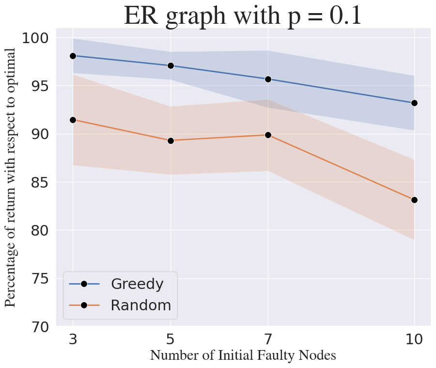
We set the discount factor and for all node pairs , and compute the infinite-horizon discounted return for the fMDP (electric network) as the fault percolation process unfolds over the network, according to the independent cascade model. We use a greedy influence maximization (IM) algorithm under the independent cascade model to identify the initial set of faulty nodes with maximum influence for fault propagation. We consider two types of random graph models to generate instances of the electric network: (i) Erdős-Rényi (ER) random graph denoted by , where represents the number of nodes and represents the edge-probability and (ii) Barabási-Albert (BA) random graph denoted by , where represents the number of nodes. We perform the following experiments to evaluate the greedy algorithm and plot the performance of greedy with respect to optimal (computed using brute-force search) along with the performance of random selection with respect to optimal in Figure 5.


Random Instances: We generate random ER networks with and set the initial number of faulty nodes to and the selection budget and run the greedy algorithm. It can be seen from Fig. 5(a) that greedy shows near-optimal performance for many instances, with an average of of the optimal.
Varying Actuator Budget: We generate random ER networks ( and ) and BA networks (). We set the initial number of faulty nodes to and run greedy for varying budgets for ER networks and for BA networks. The comparison of greedy and random selection with respect to optimal as the selection budget increases is shown in Figures 5(d), 5(g) and 5(i). It can be observed that greedy clearly outperforms random selection for both ER and BA networks, with near-optimal performance.
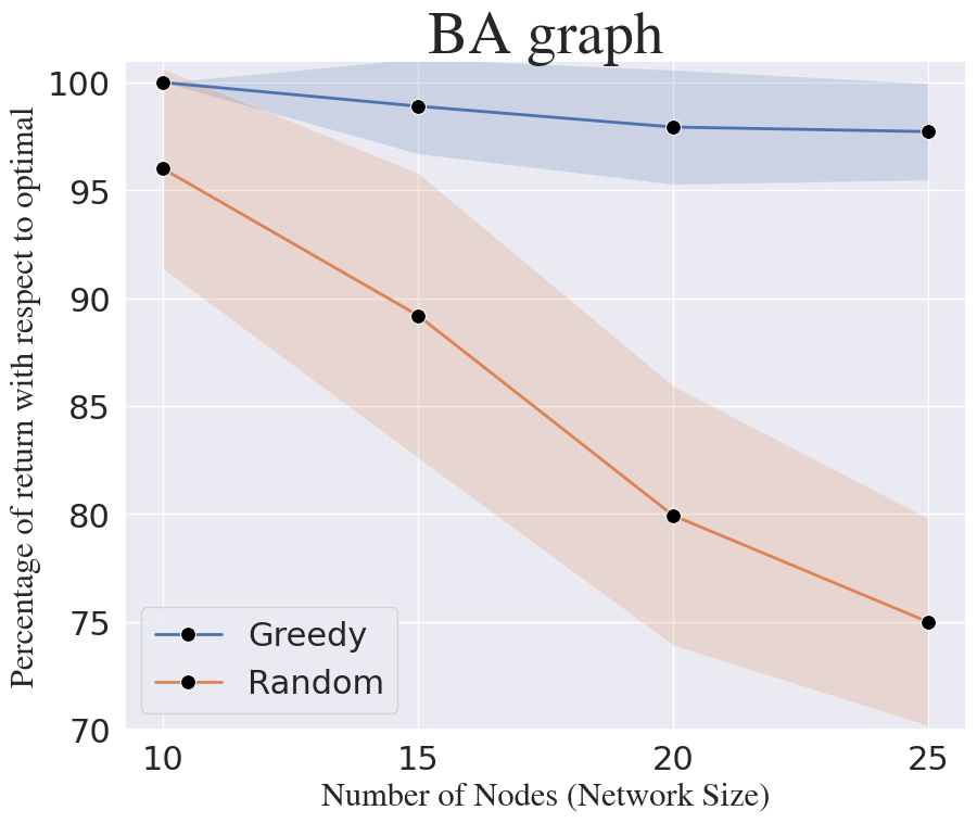
Varying Network Size: We generate random ER networks ( and ) and BA networks (). with varying network sizes, i.e., . We set the initial number of faulty nodes to and actuator selection budget to . The comparison of greedy and random selection with respect to optimal as the network size increases is shown in Figures 5(e), 5(h) and 5(k). It can be observed that greedy provides near-optimal performance for both ER and BA networks as the network size increases, while random selection performs poorly compared to greedy as the network size increases.
Varying Number of Faulty Nodes: We generate random ER networks ( and ) and BA networks (). We vary the initial number of faulty nodes and set the selection budget to . The comparison of greedy and random selection with respect to optimal as the network size increases is shown in Figures 5(f), 5(i) and 5(l). It can be observed that greedy provides near-optimal performance and outperforms random selection for various network types and sizes.
In all the above cases, the greedy algorithm provides a performance of over of the optimal. We conclude that, though the fMDP-AS problem is inapproximable to within a non-trivial factor, the greedy algorithm can provide near-optimal solutions to many instances in practice.
5.2 Evaluation on Random Instances
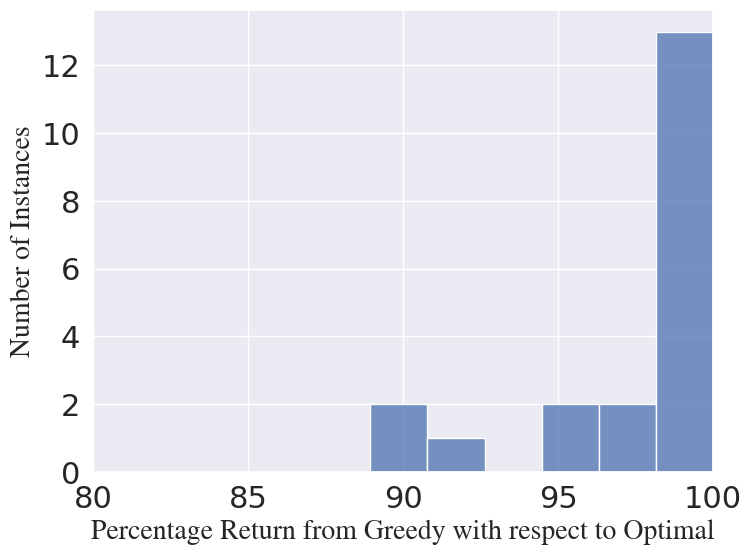
First, we evaluate the greedy algorithm for several randomly generated instances of fMDP-SS. Note that any instance of the fMDP-SS problem can be represented as a Partially Observable MDP (POMDP) to solve for the optimal policy. Hence, we use the SolvePOMDP software package [40], a Java program that can solve partially observable Markov decision processes optimally using incremental pruning [41] combined with state-of-the-art vector pruning methods [42]. We run the exact algorithm in this package to compute the optimal solution for infinite-horizon cases by setting a value function tolerance as a stopping criterion. We generate 20 instances of fMDP-SS with each instance having states ( binary state variables) and actions. The transition function for each starting state , action and ending state is a point on a probability simplex is randomly selected. The rewards for each state-action pair are randomly sampled from , with . We consider a set of 4 noise-less sensors , which can measure the states , respectively. We consider uniform sensor costs and a sensor budget of . We apply a brute-force technique by generating all possible sensor subsets of size , to compute the optimal set of sensors and compute the optimal return using the solver. We run Algorithm 1 for each of these instances to compute the return . It can be seen from Fig. 5(b) that greedy shows near-optimal performance, with an average of of the optimal.
Next, we evaluate the performance of the greedy algorithm over randomly generated instances of the fMDP-AS problem. Note that any instance of the fMDP-AS problem can be solved to find the optimal policy using an MDP solver. We apply the policy iteration algorithm to find the optimal policy and the corresponding infinite-horizon expected return using the MDPToolbox package in Python [43]. We generate 20 instances of fMDP-AS with each instance having states. We consider a set of 10 actuators with uniform selection costs and a budget of . The action space is given by , where is the joint action space corresponding to the selected actuator set. By default, there are two actions available to the agent, i.e., . Each new actuator selected corresponds to a new action variable in the joint action . The transition function for each starting state , action and ending state is a value randomly sampled over a probability simplex . The rewards for each tuple are randomly sampled from , with . We apply a brute-force technique to obtain the optimal set of actuators and compute the optimal return . We run Algorithm 1 for these instances to compute the return . It can be seen from Fig. 5(c) that greedy shows near-optimal performance, with an average of of the optimal.
6 Conclusions
In this paper, we studied the budgeted (and design-time) sensor and actuator selection problems for fMDPs, and proved that they are NP-hard in general, and there is no polynomial-time algorithm that can approximate them to any non-trivial factor of the optimal solution. Our inapproximability results directly imply that greedy algorithms cannot provide constant-factor guarantees for our problems, and that the value function of the fMDP is not submodular in the set of sensors (or actuators) selected. We explicitly show how greedy algorithms can provide arbitrarily poor performance even for very small instances of the fMDP-SS (or fMDP-AS) problems. With these results, we conclude that these problems are more difficult than other variants of sensor and actuator selection problems that have submodular objectives. Finally, we demonstrated the empirical performance of the greedy algorithm for actuator selection in electric networks and several randomly generated fMDP-SS and fMDP-AS instances and concluded that although greedy performed arbitrarily poorly for some instances, it can provide near-optimal solutions in practice. Future works on extending the results to fMDPs over finite time horizons, and identifying classes of systems that admit near-optimal approximation guarantees are of interest.
References
- [1] Chen Tessler, Yuval Shpigelman, Gal Dalal, Amit Mandelbaum, Doron Haritan Kazakov, Benjamin Fuhrer, Gal Chechik, and Shie Mannor. Reinforcement learning for datacenter congestion control. ACM SIGMETRICS Performance Evaluation Review, 49(2):43–46, 2022.
- [2] Qinghui Tang, Sandeep Kumar S Gupta, and Georgios Varsamopoulos. Energy-efficient thermal-aware task scheduling for homogeneous high-performance computing data centers: A cyber-physical approach. IEEE Transactions on Parallel and Distributed Systems, 19(11):1458–1472, 2008.
- [3] Craig Boutilier, Richard Dearden, Moisés Goldszmidt, et al. Exploiting structure in policy construction. In IJCAI, volume 14, pages 1104–1113, 1995.
- [4] Carlos Guestrin, Daphne Koller, Ronald Parr, and Shobha Venkataraman. Efficient solution algorithms for factored MDPs. Journal of Artificial Intelligence Research, 19:399–468, 2003.
- [5] Carlos Guestrin, Daphne Koller, and Ronald Parr. Multiagent planning with factored MDPs. Advances in neural information processing systems, 14, 2001.
- [6] Joelle Pineau, Geoff Gordon, and Sebastian Thrun. Point-based value iteration: An anytime algorithm for POMDPs. In IJCAI, volume 3, 2003.
- [7] Hanna Kurniawati, David Hsu, and Wee Sun Lee. SARSOP: Efficient point-based POMDP planning by approximating optimally reachable belief spaces. In Robotics: Science and systems, 2008.
- [8] Mauricio Araya-López, Vincent Thomas, Olivier Buffet, and François Charpillet. A closer look at MOMDPs. In 22nd International Conference on Tools with Artificial Intelligence, volume 2, pages 197–204. IEEE, 2010.
- [9] Haotian Zhang, Raid Ayoub, and Shreyas Sundaram. Sensor selection for Kalman filtering of linear dynamical systems: Complexity, limitations and greedy algorithms. Automatica, 78:202–210, 2017.
- [10] Lintao Ye, Nathaniel Woodford, Sandip Roy, and Shreyas Sundaram. On the complexity and approximability of optimal sensor selection and attack for Kalman filtering. IEEE Transactions on Automatic Control, 66(5):2146–2161, 2020.
- [11] Vasileios Tzoumas, Mohammad Amin Rahimian, George J Pappas, and Ali Jadbabaie. Minimal actuator placement with bounds on control effort. IEEE Transactions on Control of Network Systems, 3(1):67–78, 2015.
- [12] Wei Li, Fan Zhou, Kaushik Roy Chowdhury, and Waleed Meleis. Qtcp: Adaptive congestion control with reinforcement learning. IEEE Transactions on Network Science and Engineering, 6(3):445–458, 2018.
- [13] Hosam Rowaihy, Matthew P Johnson, Sharanya Eswaran, Diego Pizzocaro, Amotz Bar-Noy, Thomas La Porta, Archan Misra, and Alun Preece. Utility-based joint sensor selection and congestion control for task-oriented wsns. In 2008 42nd Asilomar Conference on Signals, Systems and Computers, pages 1165–1169. IEEE, 2008.
- [14] Martin Duggan, Kieran Flesk, Jim Duggan, Enda Howley, and Enda Barrett. A reinforcement learning approach for dynamic selection of virtual machines in cloud data centres. In International Conference on Innovative Computing Technology (INTECH), pages 92–97. IEEE, 2016.
- [15] Farshid Hassani Bijarbooneh, Wei Du, Edith C-H Ngai, Xiaoming Fu, and Jiangchuan Liu. Cloud-assisted data fusion and sensor selection for internet of things. IEEE Internet of Things Journal, 3(3):257–268, 2015.
- [16] Chase St Laurent and Raghvendra V Cowlagi. Coupled sensor configuration and path-planning in unknown static environments. In American Control Conference (ACC), pages 1535–1540. IEEE, 2021.
- [17] Arthur W Mahoney, Trevor L Bruns, Philip J Swaney, and Robert J Webster. On the inseparable nature of sensor selection, sensor placement, and state estimation for continuum robots or “where to put your sensors and how to use them”. In 2016 IEEE International Conference on Robotics and Automation (ICRA), pages 4472–4478, 2016.
- [18] Han-Pang Chiu, Xun S Zhou, Luca Carlone, Frank Dellaert, Supun Samarasekera, and Rakesh Kumar. Constrained optimal selection for multi-sensor robot navigation using plug-and-play factor graphs. In IEEE International Conference on Robotics and Automation (ICRA), pages 663–670, 2014.
- [19] Circuit Globe: Electric Grid. https://circuitglobe.com/electrical-grid.html.
- [20] Mahsa Ghasemi and Ufuk Topcu. Online active perception for partially observable Markov decision processes with limited budget. In Conference on Decision and Control (CDC), pages 6169–6174. IEEE, 2019.
- [21] Vikram Krishnamurthy and Dejan V Djonin. Structured threshold policies for dynamic sensor scheduling—a partially observed Markov decision process approach. IEEE Transactions on Signal Processing, 55(10):4938–4957, 2007.
- [22] Shihao Ji, Ronald Parr, and Lawrence Carin. Nonmyopic multiaspect sensing with partially observable Markov decision processes. IEEE Transactions on Signal Processing, 55(6):2720–2730, 2007.
- [23] Krithika Manohar, J Nathan Kutz, and Steven L Brunton. Optimal sensor and actuator selection using balanced model reduction. IEEE Transactions on Automatic Control, 67(4):2108–2115, 2021.
- [24] Tyler H Summers and John Lygeros. Optimal sensor and actuator placement in complex dynamical networks. IFAC Proceedings Volumes, 47(3):3784–3789, 2014.
- [25] Alexander Fuchs and Manfred Morari. Actuator performance evaluation using lmis for optimal hvdc placement. In 2013 European Control Conference (ECC), pages 1529–1534. IEEE, 2013.
- [26] A. Fuchs and M. Morari. Placement of HVDC links for power grid stabilization during transients. In 2013 IEEE Grenoble Conference, pages 1–6. IEEE, 2013.
- [27] Abolfazl Hashemi, Haris Vikalo, and Gustavo de Veciana. On the benefits of progressively increasing sampling sizes in stochastic greedy weak submodular maximization. IEEE Transactions on Signal Processing, 70:3978–3992, 2022.
- [28] Abolfazl Hashemi, Mahsa Ghasemi, Haris Vikalo, and Ufuk Topcu. Randomized greedy sensor selection: Leveraging weak submodularity. IEEE Transactions on Automatic Control, 66(1):199–212, 2020.
- [29] Daniel Golovin and Andreas Krause. Adaptive submodularity: Theory and applications in active learning and stochastic optimization. Journal of Artificial Intelligence Research, 42:427–486, 2011.
- [30] Rajiv Khanna, Ethan Elenberg, Alex Dimakis, Sahand Negahban, and Joydeep Ghosh. Scalable greedy feature selection via weak submodularity. In Artificial Intelligence and Statistics, pages 1560–1568. PMLR, 2017.
- [31] Christos H Papadimitriou and John N Tsitsiklis. The complexity of Markov decision processes. Mathematics of operations research, 12(3):441–450, 1987.
- [32] Jayanth Bhargav, Mahsa Ghasemi, and Shreyas Sundaram. On the Complexity and Approximability of Optimal Sensor Selection for Mixed-Observable Markov Decision Processes. In 2023 American Control Conference (ACC), pages 3332–3337. IEEE, 2023.
- [33] Michael R Garey. Computers and intractability: A guide to the theory of NP-Completeness. Fundamental, 1997.
- [34] David Kempe, Jon Kleinberg, and Éva Tardos. Maximizing the spread of influence through a social network. In Proceedings of the ninth ACM SIGKDD international conference on Knowledge discovery and data mining, pages 137–146, 2003.
- [35] Grant Schoenebeck and Biaoshuai Tao. Beyond worst-case (in) approximability of nonsubmodular influence maximization. ACM Transactions on Computation Theory (TOCT), 11(3):1–56.
- [36] Richard M Karp. Reducibility among combinatorial problems. Springer, 2010.
- [37] George L Nemhauser, Laurence A Wolsey, and Marshall L Fisher. An analysis of approximations for maximizing submodular set functions—i. Mathematical programming, 14(1):265–294.
- [38] Andreas Krause and Carlos Guestrin. Near-optimal observation selection using submodular functions. In AAAI, volume 7, pages 1650–1654, 2007.
- [39] Ruidong Yan, Deying Li, Weili Wu, Ding-Zhu Du, and Yongcai Wang. Minimizing influence of rumors by blockers on social networks: algorithms and analysis. IEEE Transactions on Network Science and Engineering, 7(3):1067–1078, 2019.
- [40] SolvePOMDP-a java program that solves Partially Observable Markov Decision Processes. https://www.erwinwalraven.nl/solvepomdp/.
- [41] Anthony R Cassandra, Michael L Littman, and Nevin Lianwen Zhang. Incremental pruning: A simple, fast, exact method for partially observable Markov decision processes. arXiv preprint arXiv:1302.1525, 2013.
- [42] Erwin Walraven and Matthijs Spaan. Accelerated vector pruning for optimal POMDP solvers. In Proceedings of the AAAI Conference on Artificial Intelligence, volume 31, 2017.
- [43] Markov Decision Process (MDP) Toolbox - a toolbox with classes and functions for the resolution of descrete-time Markov Decision Processes. https://pymdptoolbox.readthedocs.io/en/latest/api/mdptoolbox.html.