Optimal Regional Tracking Control of Time-Fractional Diffusion Systems
Abstract
In this paper, we aim to explore optimal regional trajectory tracking control problems of the anomalous subdiffusion processes governed by time-fractional diffusion systems under the Neumann boundary conditions. Using eigenvalue theory of the system operator and the semigroup theory, we explore the existence and some estimates of the mild solution to the considered system. An approach on finding solution to the optimal problem that minimizes the regional trajectory tracking error and the corresponding control cost over a finite space and time domain is then explored via the Hilbert uniqueness method (HUM). The obtained results not only can be directly used to investigate the systems that are not controllable on the whole domain, but also yield an explicit expression of the control signal in terms of the desired trajectory. Most importantly, it is worth noting that our results in this paper are still novel even for the special case when the order of fractional derivative is equal to one. Finally, we provide a numerical example to illustrate our theoretical results.
Index Terms:
Regional tracking control; Optimal Control; Time-fractional diffusion systems; Hilbert uniqueness method.I Introduction
During the past two decades, there is an increasing activity in the discussion of tracking problems for conventional reaction-diffusion dynamic systems, which can be divided into two steps: trajectory planning and tracking control (see e.g., the monographes [1, 2]). In these studies, the trajectory planning step attempts to generate a reference trajectory for the given desired function, while the tracking control focuses on system dynamics and hopes to design a sequence of inputs to track the pre-planned reference trajectory [3]. For the trajectory planning problems, we refer the reader to [4, 5, 6] where the flatness-based feedforward control strategies were presented or to [7] where the hardware and numerical illustrations were carried out. Moreover, to improve the accuracy in tracking control, various controller design techniques such as sliding-mode control [8], robust control [9], iterative learning control [10] and active disturbance rejection control (ADRC) [11] have been developed.
On the other hand, after the pioneering work given by Einstein in [12], it is confirmed that conventional diffusion system can well model the Brownian motion, whose mean-square displacement (MSD) is a linear function of time . However, there exist a great deal of extremely complex transport processes that is characterized by a power-law MSD relation i.e., MSD including the anomalous subdiffusion case with and the anomalous superdiffusion case with . In these anomalous situations, the usual physical laws would never be followed and the mathematical models will divert from the traditional integer-order systems to the fractional-order cases [13, 14, 15, 16]. Besides, we see that for anomalous subdiffusion process, time-fractional diffusion system has been confirmed as a powerful tool to model it [17, 18, 19]. Here the time-fractional diffusion system is a new extension model of conventional diffusion system by replacing the first order time derivative with a fractional-order derivative of order . This is due to the fact that fractional-order derivative is defined as a kind of convolution hence representing well the dynamics inheriting subdiffusive properties and moreover, the fractional-order derivative would recover the first-order derivative if it approaches to one [20]. Then, based on our previous work on trajectory planning problem of time-fractional reaction-diffusion systems [21], in this paper, we go on investigating the optimal trajectory tracking control problems of linear time-fractional diffusion systems with the Neumann boundary conditions. Further results on optimal tracking control of coupled nonlinear time-fractional diffusion systems under more general boundary conditions will be discussed in our forthcoming works.
Let be an open bounded subset of with Lipschitz continuous boundary and denote , with Herein, we consider the following time-fractional diffusion system with a Caputo fractional derivative of order :
| (1) |
where generates a strongly continuous semigroup on the Hilbert space , is a uniformly elliptic operator (see e.g., the Definition 9.2 of [22]), denotes the control inputs and represents the unit outside normal vector of the boundary . Here represents the usual Hilbert space endowed with the inner product and the norm . As cited in [23], system covers a great deal of real-world applications in a spatially inhomogeneous environment. Typical examples include the reheating processes of heterogeneous metal slabs [16] or the flow through porous media with varying sources or sinks [24] and so on.
Taking into account that not all the states of time-fractional diffusion systems are reachable in the whole domain of interest. To address this issue, regional control ideas such as regional controllability [25, 26], regional observability [27] and regional stability [28, 29] have been employed and well studied due to their advantages of offering potential to reduce computational requirements and being possible to study the systems that are not controllable on the whole domain. With these in mind, the novelty in this paper is promoting to study regional trajectory tracking control problem of the system . For this purpose, we focus on employing optimal control strategy to determine control signals by minimizing the proposed tracking cost functional. However, optimal control design for system is very challenging or even impossible due to the infinite dimensionality property of the problem. To overcome this limitation, the HUM provides an alternative approach [25, 30, 31]. In this method, dual system is selected to determine the explicit expression of optimal solution to the cost functional. To the best of our knowledge, no results are available on this topic. Most importantly, we claim that our results in this paper are still novel even for the special case when the order of fractional derivative in considered system is equal to one.
The rest of this paper is organized as follows. Some preliminary results that are useful for the study are given in Section 2. In Section 3, we present our main results on the HUM-based optimal regional trajectory tracking control strategy for time-fractional diffusion systems. This is illustrated in Section 4, where a numerical example is presented.
II Preliminaries
Definition 1
[20] Given a function , the Riemann-Liouville fractional integral of order for is as follows
| (2) |
Here
| (3) |
denotes the Euler gamma function and the right side of is pointwise defined on .
Definition 2
[20] Given a function , the Caputo fractional derivative of order for is
| (6) |
provided that the right side is pointwise defined on .
Recall that is a uniformly elliptic operator, by [32], under the Neumann boundary condition, the eigenvalue pairing with of the Sturm-Liouville problem
| (8) |
satisfies
and forms a orthonormal basis of . This is general. For example, when is a dimensional parallelepipedon, we refer the reader to Lemma 2 of [5] for a detailed expression of the corresponding eigenvalue pairing . With these, any can be expressed as
| (11) |
Then, the strongly continuous semigroup on generated by satisfies
| (14) |
Denote by and the usual Sobolev spaces (see e.g., [33]), now we are ready to give the following lemma.
Lemma 1
Let denote the solution of system for any given control . Choose a positive Lebesgue measure sub-region, we define as the corresponding Hilbert space on and set . Moreover, let be the characteristic function of given by
| (27) |
We have the following definition.
Definition 3
The considered optimal regional trajectory tracking control problem for system in at time concerns how to design controller such that starting from could reach the given target function in as close as possible along with the given trajectory within , i.e.,
| (29) |
The following lemma plays a key role for our later technical development.
III Optimal regional tracking control
The control objective of this article is the guidance of state trajectories of system along a given trajectory to reach the final target function in at time . The closer the controlled , follows the desired trajectory and the target , the better the control target is achieved.
Suppose that is an nonempty closed, convex subset of , in this section, we aim to find such that
| (38) |
where is the squared difference integrated performance functional given by
| (42) |
and , are three given constants. Here may be the equilibrium or any given target functions of system . For this purpose, since is a nonempty closed convex subset, the following lemma is necessary.
Lemma 3
Based on Lemma 3, we get that the unique solution of the optimization problem can be characterized by
| (46) |
and more precisely,
| (47) |
after a simple duality derivation. Here
| (51) |
denotes the adjoint operator of and . Further, to simplify above equation , let us introduce the following adjoint system
| (52) |
where is the adjoint operator of and is an operator given by as in property 2.7 of [36] satisfying
| (53) |
| (54) |
as a consequence of Eq. and Eq.. To establish the existence of a unique solution to system , it is supposed that the eigenvalue pairing of operator under the Neumann boundary conditions is , where also forms a orthonormal basis of . Recall from Lemma 1 and the Lemma 1 of [25], given any and , based on the property of operator , we have the following result.
Lemma 4
Given any and , if conditions of Lemma 1 are satisfied, then system admits a unique mild solution as follows
| (57) |
where
| (59) |
for any .
Proof:
In what follows, we proceed to simplify based on the adjoint system .
Indeed, for the first term of above equation , using Lemma 2, it yields that
Since is a uniformly elliptic operator, for any one has [22]
| (65) |
Then, using formula , we have
This, together with the boundary conditions of considered systems, yields that
Therefore, the optimality condition can be simplified to
| (69) |
for all
Now we summarize the following result and omit the detailed proof.
Theorem 1
Given any target trajectory and the target function , the optimal problem admits a unique optimal solution that is determined by the system and the adjoint system satisfying the variational inequality .
In particular, when , since holds true if
| (71) |
Furthermore, in order to obtain the optimal control in feedback form, according to Lemma 1, and , we have
Since for any given let . We have
| (74) |
where
and
Then, the iterative methods can be used to obtain the values of , . With this, we therefore, get that the unique optimal solution to system can be governed by
| (78) |
This allows us to give the explicit expression of the designed optimal controller and at the same time, to minimize the tracking cost functional .
IV Numerical example
This section aims to present a numerical simulation illustrating our obtained results. For the sake of simplicity, we let and claim that the higher-dimensional spatial domain case can be considered in a similar way.
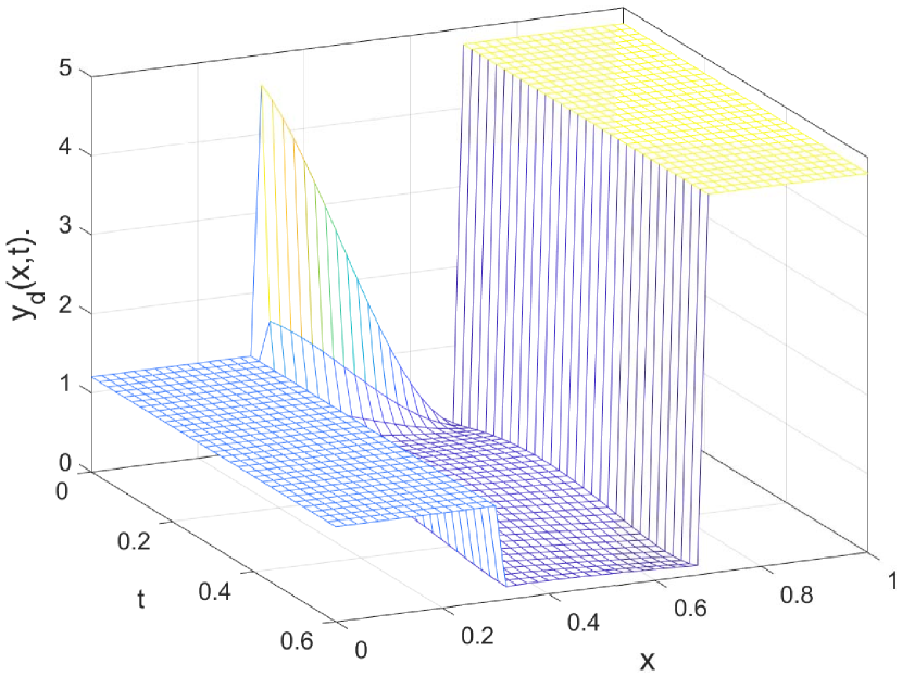
(a) The desired trajectory .
(b) The evolution of .
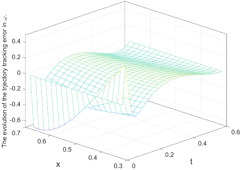
(c) The tracking error in .
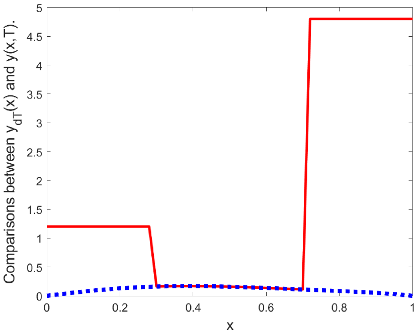
(d) Comparisons between and in .
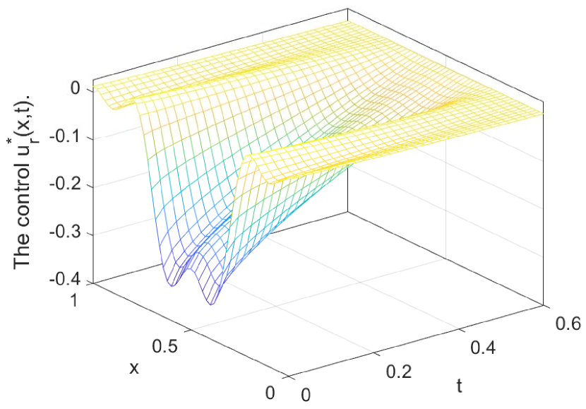
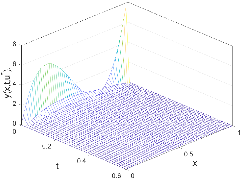
(e) The optimal control .
Let us consider the following example
| (79) |
Obviously, , and is a uniformly elliptic operator. Under the Neumann boundary conditions for all the eigenvalue paring of operator satisfies [5]
| (81) |
and
| (85) |
Then, the corresponding strongly continuous semigroup satisfies
| (87) |
By Lemma 1, it yields that
| (89) |
and
Let the subregion and the desired trajectory be
| (93) |
One has
In what follows, we aim to solve the following optimal control problem
| (96) |
with
| (100) |
According to Theorem 1, the optimal control problem admits a unique optimal solution governed by
| (102) |
Moreover, to illustrate the effectiveness of our results, we set
| (106) | |||
| (111) |
and then plot Figures 1 , which show how closely does the state evolution track along the desired trajectory and the final state reach the target function in with the error
| (114) |
The corresponding optimal solution of the optimal control problem is depicted in Figure 1 with the costs .
V Conclusion
Sufficient and necessary conditions for optimal regional trajectory tracking control problem of linear time-fractional diffusion systems are obtained in this paper by using the HUM. The obtained results not only can be used directly to discuss the systems that are not controllable on the whole domain, but also yield an explicit expression of the control signal in terms of the desired trajectory and minimize the proposed tracking cost functional as well. This is very appealing in practical applications and pose many new theoretically challenges at the same time. Moreover, we claim that the main results in this paper can be extended to more complex fractional-order distributed parameter systems (see those in [37] for example)and various open questions such as optimal actuation configuration problems for regional tracking control of the coupled nonlinear space-time fractional diffusion systems are still open.
References
- [1] J. Lber, Optimal Trajectory Tracking of Nonlinear Dynamical Systems, Springer, 2017.
- [2] T. Meurer, Control of Higher–Dimensional PDEs: Flatness and Backstepping Designs, Springer Science & Business Media, 2012.
- [3] Y. Choi, W. K. Chung, PID Trajectory Tracking Control for Mechanical Systems, Springer Science & Business Media, 2004.
- [4] T. Meurer, A. Kugi, Trajectory planning for boundary controlled parabolic PDEs with varying parameters on higher-dimensional spatial domains, IEEE Transactions on Automatic Control 54 (8) (2009) 1854–1868.
- [5] T. Meurer, Flatness-based trajectory planning for diffusion–reaction systems in a parallelepipedon—a spectral approach, Automatica 47 (5) (2011) 935–949.
- [6] G. Freudenthaler, T. Meurer, PDE-based multi-agent formation control using flatness and backstepping: Analysis, design and robot experiments, Automatica 115 (2020) 108897.
- [7] K. L. Moore, Y. Chen, Z. Song, Diffusion-based path planning in mobile actuator-sensor networks (MAS-net): some preliminary results, Proceedings of SPIE - The International Society for Optical Engineering 5421 (2004) 58–69.
- [8] A. Pisano, Y. Orlov, E. Usai, Tracking control of the uncertain heat and wave equation via power-fractional and sliding-mode techniques, Siam Journal on Control and Optimization 49 (2) (2011) 363–382.
- [9] Y. Weng, X. Gao, Data-driven robust output tracking control for gas collector pressure system of coke ovens, IEEE Transactions on Industrial Electronics 64 (5) (2017) 4187–4198.
- [10] J. Kang, A newton-type iterative learning algorithm of output tracking control for uncertain nonlinear distributed parameter systems, in: Proceedings of the 33rd Chinese Control Conference. IEEE, 2014, pp. 8901–8905.
- [11] H. Zhou, B. Guo, S. Xiang, Performance output tracking for multidimensional heat equation subject to unmatched disturbance and noncollocated control, IEEE Transactions on Automatic Control 65 (5) (2019) 1940–1955.
- [12] A. Einstein, ber die von der molekularkinetischen Theorie der Wrme geforderte Bewegung von in ruhenden Flssigkeiten suspendierten Teilchen, Annalen der Physik 322 (1905) 549–560.
- [13] F. Ge, Y. Chen, Event-triggered boundary feedback control for networked reaction-subdiffusion processes with input uncertainties, Information Sciences 476 (2019) 239–255.
- [14] F. Ge, Y. Chen, Observer-based event-triggered control for semilinear time-fractional diffusion systems with distributed feedback, Nonlinear Dynamics 99 (2) (2020) 1089–1101.
- [15] V. Uchaikin, R. Sibatov, Fractional Kinetics in Solids: Anomalous Charge Transport in Semiconductors, Dielectrics and Nanosystems, World Science, 2013.
- [16] F. Ge, Y. Chen, C. Kou, Regional Analysis of Time-Fractional Diffusion Processes, Springer, 2018.
- [17] R. Metzler, J. Klafter, The random walk’s guide to anomalous diffusion: A fractional dynamics approach, Physics Reports 339 (1) (2000) 1–77.
- [18] F. Ge, Y. Chen, C. Kou, I. Podlubny, On the regional controllability of the sub-diffusion process with Caputo fractional derivative, Fractional Calculus and Applied Analysis 19 (5) (2016) 1262–1281.
- [19] F. Ge, T. Meurer, Y. Chen, Mittag-Leffler convergent backstepping observers for coupled semilinear subdiffusion systems with spatially varying parameters, Systems & Control Letters 122 (2018) 86–92.
- [20] A. A. Kilbas, H. M. Srivastava, J. J. Trujillo, Theory and Applications of Fractional Differential Equations, Elsevier Science Limited, 2006.
- [21] F. Ge, T. Meurer, Trajectory planning for semilinear time-fractional reaction-diffusion systems under Robin boundary conditions, The 21st IFAC World Congress, Berlin, Germany, July 12-17, 2020. (Accepted to appear).
- [22] M. Renardy, R. C. Rogers, An introduction to Partial Differential Equations, Springer Science & Business Media, 2006.
- [23] H. Sun, Y. Zhang, D. Baleanu, W. Chen, Y. Chen, A new collection of real world applications of fractional calculus in science and engineering, Communications in Nonlinear Science and Numerical Simulation 64 (2018) 213–231.
- [24] V. V. Uchaikin, R. T. Sibatov, Fractional theory for transport in disordered semiconductors, Communications in Nonlinear Science and Numerical Simulation 13 (4) (2008) 715–727.
- [25] F. Ge, Y. Chen, C. Kou, Regional controllability analysis of fractional diffusion equations with Riemann–Liouville time fractional derivatives, Automatica 76 (2017) 193–199.
- [26] F. Ge, Y. Chen, C. Kou, Regional gradient controllability of sub-diffusion processes, Journal of Mathematical Analysis and Applications 440 (2) (2016) 865–884.
- [27] F. Ge, Y. Chen, C. Kou, On the regional gradient observability of time fractional diffusion processes, Automatica 74 (2016) 1–9.
- [28] W. Kang, E. Fridman, Constrained control of 1-D parabolic PDEs using sampled in space sensing and actuation, Systems & Control Letters 140 (2020) 104698.
- [29] F. Ge, Y. Chen, Regional output feedback stabilization of semilinear time-fractional diffusion systems in a parallelepipedon with control constraints, International Journal of Robust and Nonlinear Control 30 (9) (2020) 3639–3652.
- [30] J. L. Lions, Optimal Control of Systems Governed by Partial Differential Equations, Vol. 170, Springer Verlag, 1971.
- [31] R. Glowinski, J. L. Lions, J. He, Exact and Approximate Controllability for Distributed Parameter Systems: A Numerical Approach, Cambridge University Press, 2008.
- [32] R. Courant, D. Hilbert, Methods of mathematical physics, Vol. 1, CUP Archive, 1966.
- [33] R. A. Adams, J. J. Fournier, Sobolev Spaces, Vol. 140, Academic Press, 2003.
- [34] K. Sakamoto, M. Yamamoto, Initial value/boundary value problems for fractional diffusion-wave equations and applications to some inverse problems, Journal of Mathematical Analysis and Applications 382 (1) (2011) 426–447.
- [35] F. Ge, Y. Chen, Optimal vaccination and treatment policies for regional approximate controllability of the time-fractional reaction–diffusion SIR epidemic systems, ISA transactions (2021) In Press. DOI: 10.1016/j.isatra.2021.01.023.
- [36] M. Klimek, On Solutions of Linear Fractional Differential Equations of A Variational Type, Publishing Office of Czestochowa University of Technology, 2009.
- [37] F. Ge, Y. Chen, C. Kou, Cyber-physical systems as general distributed parameter systems: three types of fractional order models and emerging research opportunities, IEEE/CAA Journal of Automatica Sinica 2 (4) (2015) 353–357.