Optimal ratcheting of dividends in a Brownian risk model
Abstract
We study the problem of optimal dividend payout from a surplus process governed by Brownian motion with drift under the additional constraint of ratcheting, i.e. the dividend rate can never decrease. We solve the resulting two-dimensional optimal control problem, identifying the value function to be the unique viscosity solution of the corresponding Hamilton-Jacobi-Bellman equation. For finitely many admissible dividend rates we prove that threshold strategies are optimal, and for any finite continuum of admissible dividend rates we establish the -optimality of curve strategies. This work is a counterpart of [2], where the ratcheting problem was studied for a compound Poisson surplus process with drift. In the present Brownian setup, calculus of variation techniques allow to obtain a much more explicit analysis and description of the optimal dividend strategies. We also give some numerical illustrations of the optimality results.
1 Introduction
The identification of the optimal way to pay out dividends from a surplus
process to shareholders is a classical topic in actuarial science and
mathematical finance. There is a natural trade-off between paying out gains as
dividends to shareholders early and at the same time leaving sufficient
surplus in order to safeguard future adverse developments and avoid ruin.
Depending on risk preferences, the concrete situation and the simultaneous
exposure to other risk factors such a problem can be formally stated in
various different ways in terms of objective functions and constraints. In
this paper we would like to follow the actuarial tradition of considering the
surplus process as the free capital in an insurance portfolio at any point in
time, and the goal is to maximize the expected sum of discounted dividend
payments that can be paid until the surplus process goes below 0 (which is
called the time of ruin). In such a formulation, the problem goes back to de
Finetti [15] and Gerber [18], and has since then been studied
in many variants concerning the nature of the underlying surplus process and
constraints on the type of admissible dividend payment strategies, see
e.g. Albrecher & Thonhauser [4] and Avanzi [8] for an
overview. From a mathematical perspective, the problem turns out to be quite
challenging, and was cast into the framework of modern stochastic control
theory and the concept of viscosity solutions for corresponding
Hamilton-Jacobi-Bellman equations over the last years, cf. Schmidli
[25] and Azcue & Muler [10].
Among the variants of the general problem is to look for the optimal dividend
payment strategy if the rate at which dividends are paid can never be reduced.
This ratcheting constraint has often been brought up by practitioners
and is in part motivated by the psychological effect that shareholders are
likely to be unhappy about a reduction of dividend payments over time (see
e.g. Avanzi et al. [9] for a discussion). One crucial question in this
context is how much of the expected discounted dividends until ruin is lost if
one respects such a ratcheting constraint, if that ratcheting is done in an
optimal way. A first step in that direction was done in Albrecher et
al. [3], where the consequences of ratcheting were studied under the
simplifying assumption that a dividend rate can be fixed in the beginning and
can be augmented only once during the lifetime of the process (concretely,
when the surplus process hits some optimally chosen barrier for the first
time). The analysis in that paper was both for a Brownian surplus process as
well as for a surplus process of compound Poisson type. In our recent paper
[2], we then provided the analysis and solution for the general
ratcheting problem for the latter compound Poisson process, and it turned out
that the optimal ratcheting dividend strategy does not lose much efficiency
compared to the unconstrained optimal dividend payout performance, and also
that the one-step ratcheting strategy studied earlier compares remarkably well
to the overall optimal ratcheting solution. In this paper we would like to
address the general ratcheting problem for the Brownian risk model. Such a
model can be seen as a diffusion approximation of the compound Poisson risk
model, but is also interesting in its own right. In particular, the fact that
ruin with zero initial capital is immediate often leads to a more amenable
analysis of stochastic control problems. In addition, the convergence of
optimal strategies from a compound Poisson setting to the one for the
diffusion approximation can be quite delicate, see e.g. Bäuerle
[12], see also Cohen and Young [13] for a recent
convergence rate analysis of simple uncontrolled ruin probabilities towards
its counterparts for the diffusion limit.
On the mathematical level, the general ratcheting formulation leads to a fully
two-dimensional stochastic control problem with all its related challenges,
and it is only recently that in the context of insurance risk theory some
first two-dimensional problems became amenable for analysis, see
e.g. Albrecher et al. [1], Gu et al. [22], Grandits
[21] and Azcue et al. [11]. In the present contribution we
would like to exploit the more amenable nature of the ratcheting problem in
the diffusion setting that push the analysis considerably further than was
possible in [2]. In particular, we will use calculus of variation
techniques to identify quite explicit formulas for the candidates of optimal
strategies and provide various optimality results.
We would like to mention that optimal ratcheting strategies have been
investigated in the framework of lifetime consumption in the mathematical
finance literature, see e.g. Dybvig [16], Elie and Touzi
[17], Jeon et al. [23] and more recently Angoshtari et
al. [5]. However, the concrete model setup and correspondingly also
the involved techniques are quite different to the one of the present paper.
The remainder of the paper is organized as follows. Section
2 introduces the model and the detailed
formulation of the problem. It also provides some first basic results on
properties of the value function under consideration. Section
3 derives the Hamilton-Jacobi-Bellman
equations and characterization theorems for the value function for both a
closed interval as well as a finite discrete set of admissible dividend
payment rates. In Section 4 we prove that the optimal
value function of the problem for discrete sets convergences to the one for a
continuum of admissible dividend rates as the mesh size of the finite set
tends to zero. In Section 5 we show that for finitely
many admissible dividend rates, there exists an optimal strategy for which the
change and non-change regions have only one connected component (this
corresponds to the extension of one-dimensional threshold strategies to the
two-dimensional case). We also provide an implicit equation defining the
optimal threshold function for this case. Subsequently, we turn to the case of
a continuum of admissible dividend rates and use calculus of variation
techniques to identify the optimal curve splitting the state space into a
change and a non-change region as the unique solution of an ordinary
differential equation. We show that the corresponding dividend strategy is
-optimal, in the sense that there exists a known sequence of
curves such that the corresponding value functions converge uniformly to the
optimal value function of the problem. Section 6
contains a numerical illustration of the optimal strategy and its performance
relative to the one of for the unconstrained dividend problem and the one
where the dividend rate can only be increased once. Section 7
concludes.
Some technical proofs are delegated to an appendix.
2 Model and basic results
Assume that the surplus process of a company is given by a Brownian motion with drift
where is a standard Brownian motion, and are given constants. Let be the complete probability space generated by the process .
The company uses part of the surplus to pay dividends to the shareholders with rates in a set , where is the maximum dividend rate possible. Let us denote by the rate at which the company pays dividends at time . Given an initial surplus and a minimum dividend rate at , a dividend ratcheting strategy is given by and it is admissible if it is non-decreasing, right-continuous, adapted with respect to the filtration and it satisfies for all . The controlled surplus process can be written as
| (1) |
Define as the set of all admissible dividend ratcheting strategies with initial surplus and minimum initial dividend rate . Given , the value function of this strategy is given by
where and is the ruin time. Hence, for any initial surplus and initial dividend rate , our aim is to maximize
| (2) |
It is immediate to see that for all
Remark 2.1
The dividend optimization problem without the ratcheting constraint, that is where the dividend strategy is not necessarily non-decreasing, was studied intensively in the literature (see e.g. Gerber and Shiu [19]). Unlike the ratcheting optimization problem, this non-ratcheting problem is one-dimensional. If denotes its optimal value function, then clearly for all and . The function is increasing, concave, twice continuously differentiable with and ; so it is Lipschitz with Lipschitz constant
The following Lemma states the dynamic programming principle, its proof is similar to the one of Lemma 1.2 in Azcue and Muler [10].
Lemma 2.1
Given any stopping time , we can write
We now state a straightforward result regarding the boundedness and monotonicity of the optimal value function.
Proposition 2.2
The optimal value function is bounded by , non-decreasing in and non-increasing in
Proof. Since the discounted value of paying the maximum rate up to infinity is we conclude the boundedness result.
On the one hand is non-increasing in because given
we have for any
. On the other hand, given and an admissible ratcheting
strategy for any , let us define as until the ruin time of the
controlled process with , and pay the
maximum rate afterwards. Thus, and
we have the result.
The Lipschitz property of the function introduced in Remark 2.1 can now be used to prove a first result on the regularity of the function
Proposition 2.3
There exists a constant such that
for all and with
The proof is given in the appendix.
3 Hamilton-Jacobi-Bellman equations
In this section we introduce the Hamilton-Jacobi-Bellman (HJB) equation of the ratcheting problem for , when is either a closed interval or a finite set. We show that the optimal value function defined in (2) is the unique viscosity solution of the corresponding HJB equation with boundary condition when goes to infinity, where
First, consider the case . In this case, the unique admissible strategy consists of paying a constant dividend rate up to the ruin time. Correspondingly, the value function is the unique solution of the second order differential equation
| (3) |
with boundary conditions and The solutions of (3) are of the form
| (4) |
where and are the roots of the characteristic equation
associated to the operator , that is
| (5) |
In the following remark, we state some basic properties of and
Remark 3.1
We have that
-
1.
if and if, and only if,
-
2.
and so
The solutions of with boundary condition are of the form
| (6) |
And finally, the unique solution of with boundary conditions and corresponds to so that
| (7) |
We have that is increasing and concave.
Remark 3.2
3.1 Hamilton-Jacobi-Bellman equations for closed intervals
Let us now consider the case with The HJB equation associated to (2) is given by
| (8) |
We say that a function is (2,1)-differentiable if is continuously differentiable and is continuously differentiable.
Definition 3.1
(a) A locally Lipschitz function where is a viscosity supersolution of (8) at , if any (2,1)-differentiable function with such that reaches the minimum at satisfies
The function is called a test function for supersolution at .
(b) A function is a viscosity subsolution of (8) at , if any (2,1)-differentiable function with such that reaches the maximum at satisfies
The function is called a test function for subsolution at .
(c) A function which is both a supersolution and subsolution at is called a viscosity solution of (8) at .
Remark 3.3
Note that, by (2), for all , so in order to simplify the notation we define
We first prove that is a viscosity solution of the corresponding HJB equation.
Proposition 3.1
is a viscosity solution of (8) in .
The proof is given in the appendix.
Note that by definition of ratcheting corresponds to the value function of the strategy that constantly pays dividends at rate , with initial surplus . So, by (7),
| (9) |
Let us now state the comparison result for viscosity solutions.
Lemma 3.2
Assume that (i) is a viscosity subsolution and is a viscosity supersolution of the HJB equation (8) for all and for all with , (ii) and are non-decreasing in the variable and Lipschitz in , and (iii) , . Then in
The proof is given in the appendix.
The following characterization theorem is a direct consequence of the previous lemma, Remark 3.2 and Proposition 3.1.
Theorem 3.3
The optimal value function is the unique function non-decreasing in that is a viscosity solution of (8) in with and for
From Definition 2, Lemma 3.2, and Remark 3.2 together with Proposition 3.1, we also get the following verification theorem.
Theorem 3.4
Consider and consider a family of strategies
If the function is a viscosity supersolution of the HJB equation (8) in with and then is the optimal value function . Also, if for each there exists a family of strategies such that is a viscosity supersolution of the HJB equation (8) in with and , then is the optimal value function .
3.2 Hamilton-Jacobi-Bellman equations for finite sets
Let us now consider the case
where . Note that We simplify the notation as follows:
The Hamilton-Jacobi-Bellman equation associated to (10) is given by
| (11) |
As in the continuous case we have that is the viscosity solution of the corresponding HJB equation. Let us introduce the definition of a viscosity solution in the one-dimensional case.
Definition 3.2
(a) A locally Lipschitz function is a viscosity supersolution of (11) at if any twice continuously differentiable function with such that reaches the minimum at satisfies
The function is called a test function for supersolution at .
(b) A function is a viscosity subsolution of (11) at if any twice continuously differentiable function with such that reaches the maximum at satisfies
The function is called a test function for subsolution at .
(c) A function which is both a supersolution and subsolution at is called a viscosity solution of (11) at .
The following characterization theorem is the analogue of Theorem 3.3 for finite sets; the proof is similar and simpler than the one in the continuous case.
Theorem 3.5
The optimal value function for is the unique viscosity solution of the associated HJB equation (11) with boundary condition and
We also have the alternative characterization theorem.
Theorem 3.6
The optimal value function for is the smallest viscosity supersolution of the the associated HJB equation (11) with boundary condition at and limit greater than or equal to as goes to infinity.
Remark 3.4
The function has the closed formula given by (7) for By the previous theorem, once is known, the optimal value function can be obtained recursively as the solution of the obstacle problem of finding the smallest viscosity supersolution of the equation above the obstacle .
4 Convergence of the optimal value functions from the discrete to the continuous case
In this section we prove that the optimal value functions of finite ratcheting strategies approximate the optimal value function of the continuous case as the mesh size of the finite sets goes to zero.
Consider for , a sequence of sets (with elements) of the form
satisfying , and mesh-size as goes to infinity.
Let us extend the definition of to the function as
| (12) |
where
| (13) |
We will prove that for any and we will study the uniform convergence of this limit.
Since , there exists the limit function
| (14) |
Later on, we will show that . Note that is non-increasing in with , and non-decreasing in with . With the same proof the one for Proposition 6.1 of [2], we have the following proposition:
Proposition 4.1
The sequence converges uniformly to
With this, we can obtain the main result of this section.
Theorem 4.2
The function defined in (14) is the optimal value function .
Proof. Note that is a limit of value functions of admissible strategies, so in order to satisfy the assumptions of Theorem 3.4, it remains to see that is a viscosity supersolution of (8) at any point with in the viscosity sense because is non-increasing in ; so it is sufficient to show that in the viscosity sense. Let be a test function for viscosity supersolution of (8) at , i.e. a (2,1)-differentiable function with
| (15) |
In order to prove that , consider now, for small enough,
Given let us consider as defined in (13),
and
Since and, from Proposition 4.1, and , we also have that because
and then
Note that is a test function for viscosity supersolution of in Equation (11) at the point because
And so
Since , as and is (2,1)-differentiable, one gets
Finally, as
and as , we obtain that and the result follows.
5 The optimal strategies
We show first that, regardless whether is finite or an interval with , the optimal strategy for sufficiently small is to immediately start paying dividends at the maximum rate .
Proposition 5.1
If , then for any
Proof. If we call then we know that . Since and , then by Theorem 3.3 and Theorem 3.5 it is enough to prove that for But, by (7) and (5)
for .
Remark 5.1
The proof of the previous proposition also shows that if there exists a and such that for , then and so for any
Let us first address the case of with . We introduce the concept of strategies with a threshold structure for each level and prove that there exists an optimal dividend payment strategy and has this form. Later we extend the concept of strategies with this type of structure to the case by means of a curve in the state space and look for the curve which maximizes the expected discounted cumulative dividends.
5.1 Optimal strategies for finite sets
Take with Since for the optimal value function is a viscosity solution of (11), there are values of where and values of where We look for the simplest dividend payment strategies, those whose value functions are solutions of for and for with some . We will show in this subsection that the optimal value function comes from such types of strategies. More precisely, take and a function ; we define a threshold strategy by backward recursion, it is a stationary strategy (which depends on both the current surplus and the implemented dividend rate )
| (16) |
as follows:
-
•
If , pay dividends with rate up to the time of ruin, that is .
-
•
If and follow
-
•
If and pay dividends with rate as long as the surplus is less than up to the ruin time; if the current surplus reaches before the time of ruin, follow . More precisely
where is the first time at which the surplus reaches
Let us call the value the threshold at dividend rate level and the threshold function. The value function of the stationary strategy is defined as
| (17) |
Note that only depends on for , and for
Proposition 5.2
We have the following recursive formula for :
for , where
Proof. We have that for
because the stationary strategy pays
when the current surplus is in . Also
because ruin is immediate at , and by definition From
(6), we get the result.
Let us now look for the maximum of the value functions among all the possible threshold functions , and denote by the optimal threshold function. From Proposition 5.1, for , so that from now on we only consider the case
Since the function is known, there are two ways to solve this optimization problem (using a backward recursion). We will study the problem using both of them.
-
1.
The first approach consists of seeing the optimization problem as a sequence of one-dimensional optimization problems, that is obtaining the maximum for . If and are known for , then from Proposition 5.2 we can obtain
(18) Note that
because , so exists.
-
2.
As a second approach, one can view the optimization problem as a backward recursion of obstacle problems (see Remark 3.4 ). If and are known for , we look for the smallest solution of the equation in with boundary condition above Then
(19) By (6), the solutions of the equation in with boundary condition are of the form
Hence is increasing in and for , and so there exists an such that
because .
Remark 5.2
In the second approach, we can see as the smallest such that and coincide; more precisely , for and for . Note that and is locally convex at . By the recursive construction, this implies that is infinitely continuously differentiable at all and continuously differentiable at the points for
Lemma 5.3
is an increasing concave function. If , is increasing, and is concave in and convex in with
In the case we have that ; in the case we have that if and only if
Proof. We have that
and
if and only if . The result follows from Definition
5.
In the next theorem, we show that there exists an optimal strategy and it is of threshold type.
Theorem 5.4
If is the optimal threshold function, then is the optimal function defined in (2) for .
Proof. By definition Assuming that for , by Theorem 3.5, it is enough to prove that is a viscosity solution of (11). Since by construction , it remains to be seen that for . By Remark 5.2, is continuously differentiable and it is piecewise infinitely differentiable in open intervals in which it solves for some By the definition of a viscosity solution, it is enough to prove the result in these open intervals. For in these open intervals,
if and only if There exists and some such that in and then
If , for , by Remark 5.3, is concave and so and we have the result.
We need to prove that for By induction
hypothesis, we know that for . In the case that
it is straightforward; in the case
that , it is enough to prove it in the
interval . But ,
and by Lemma 5.3 is
either increasing, or decreasing, or decreasing and then increasing in the
interval , so that we have the result.
Taking the derivative in (18) with respect to , we get implicit equations for the optimal threshold strategy.
Proposition 5.5
satisfies the implicit equation
for
Remark 5.3
Given , we have defined in (16) a threshold strategy , where for . We can extend this threshold strategy to
| (20) |
as follows:
-
•
If and , pay dividends with rate while the current surplus is less than up to the time of ruin. If the current surplus reaches before the time of ruin, follow .
-
•
If and for , follow
The value function of the stationary strategy is defined as
| (21) |
5.2 Curve strategies and the optimal curve strategy
As it is typical for these type of problems, the way in which the optimal value function solves the HJB equation (8) suggests that the state space is partitioned into two regions: a non-change dividend region in which the dividends are paid at constant rate and a change dividend region in which the rate of dividends increases. Roughly speaking, the region consists of the points in the state space where and and consists of the points where . We introduce a family of stationary strategies (or limit of stationary strategies) where the change and non-change dividend payment regions are connected and split by a free boundary curve. This family of strategies is the analogue to the threshold strategies for finite introduced in Section 5.1.
Let us consider the set
| (22) |
In the first part of this subsection, we define the -value function associated to a curve
for , and we will see that, in some sense, is a (limit) value function of the strategy which pays dividends at
constant rate in the case that and otherwise increases the rate
of dividends. So the curve splits the state space
into two connected
regions: where dividends are paid with
constant rate, and where the dividend
rate increases. In the second part of the subsection we then will look for the
that maximizes the -value
function , using calculus of variations.
Let us consider the following auxiliary functions ,
| (23) |
Both and are not defined in so we extend the definition as
and
In order to define the -value function in the non-change region , we will define and study in the next technical lemma the functions and for any .
Lemma 5.6
Given , the unique continuous function which satisfies for any that
with boundary conditions , and at the points of continuity of is given by
| (24) |
where
| (25) |
Moreover, satisfies , is differentiable and satisfies
| (26) |
at the points where is continuous.
Proof. Since and , we can write by (6)
where should be defined in such a way that (because and
at the points of continuity of . Hence,
Solving this ODE with boundary condition , we get
the result.
Given , we define the -value function
| (27) |
where is defined in Lemma 5.6 and
| (28) |
in the case that and .
In the next propositions we will show that the -value function is the value function of an extended threshold strategy in the case that is a step function, and the limit of value functions of extended threshold strategies in the case that .
Proposition 5.7
Given and the corresponding extended threshold strategy defined in Remark 5.3, let us consider the associated step function defined as
Then the stationary value function of the extended threshold strategy is given by
Proof. The stationary value function is continuous and satisfies
for , , and for
. Also the right-hand derivatives for So, by Lemma
5.6, we obtain that if If the result follows from the
definition of .
In the previous proposition we showed that in the case where is the
associated step function of , the stationary strategy consists of increasing immediately the divided rate from
to for , paying dividends at rate
until either reaching the curve or ruin (whatever
comes first) for , and paying dividends at rate
until the time of ruin for .
In the next proposition we show that for any , the -value function is the limit of value functions of extended threshold strategies.
Proposition 5.8
Given , there exists a sequence of right-continuous step functions such that converges uniformly to .
Proof. Since is a Riemann integrable càdlàg function, we can approximate it uniformly by right-continuous step functions. Namely, take a sequence of finite sets with , and consider the right-continuous step functions
such that . We have that uniformly,
and so both and uniformly.
We now look for the maximum of among . We will show that if there exists a function such that
| (29) |
then for all and This follows from (24) and the next lemma, in which we prove that the function which maximizes (29) also maximizes for any
Lemma 5.9
Proof. Given we can write
So
Assuming that exists, we will use calculus of variations to obtain an implicit equation for . First we prove the following technical lemma.
Lemma 5.10
For any we have
Proof.
Let us now find the implicit equation for
Proposition 5.11
Proof. Consider any function with then
Taking the derivative with respect to and taking , we get
And so,
Since this holds for any with , we obtain that for any
Using Lemma 5.10, we get the implicit equation for . By definition . Now take , and the constant step function defined as where satisfies
Then
From now on, we extend the definition of to as
Since , we get from Proposition 5.11
| (30) |
and since for , we obtain that
In the next proposition we show that, under some assumptions, the function is the unique solution of the first order differential equation
| (31) |
with boundary condition (30).
Proposition 5.12
Proof. From (26), we have
| (33) |
By Assumption (32), the function
satisfies
Hence, from (33), we have that is differentiable and we
get the differential equation (31) for
. We obtain by a recursive argument that is
infinitely differentiable.
In the next proposition, we state that the value function satisfies a smooth-pasting property on the smooth free-boundary curve
We also show that, under some conditions, is the unique continuous function such that the associated -value function satisfies the smooth-pasting property at the curve .
Proposition 5.13
Proof. Let us define for and the function
| (34) |
where is a function with . Note that satisfies for all and . We have,
If is differentiable,
| (35) |
and
In the case that , take as defined in (24), by (26) and Proposition 5.11, we obtain . Since for and for , we get for and so . From (35), we get
Conversely, note that there exists such that defined in (34) for ; the existence of implies that is differentiable. Hence,
which implies
Also,
implies
Since , both and
satisfy the same equation and so they coincide.
In the next proposition, we show more regularity for in the case that is increasing.
Proposition 5.14
Proof. It is enough to prove that for . We have
And so,
5.3 Optimal strategies for the closed interval
First in this section, we give a verification result in order to check if a -value function is the optimal value function . Our conjecture is that the solution of (31) with boundary condition (30) exists and is non-decreasing in , and that coincides with , so that there exists an optimal curve strategy.
Using Proposition 5.1, we know that the conjecture holds
for taking In the
case that , we will show that exists and is increasing and for
for small enough.
We were not able to prove the conjecture in the general case, although it
holds in our numerical explorations (see Section 6).
However, we will prove that the -value functions are
-optimal in the following sense: There exists a sequence
such that converges uniformly to the
optimal value function .
We state now a verification result for checking whether the -value function with continuous is the optimal value function . In this verification result it is not necessary to use viscosity solutions because the proposed value function solves the HJB equation in a classical way. We will check these verification conditions for the limit value function associated to the unique solution of (31) with boundary condition (30) (if it exists).
Proposition 5.15
If there exists a smooth function such that the -value function is (2,1)-differentiable and satisfies
then .
Proof. We have that for because is concave and Since for ; for and ; by Theorem 3.3 it is sufficient to prove that for . In this case, we have that
satisfies , and also either or So, we obtain and then
Next we see that there exists a unique solution of (31) with boundary condition (30) at least in for some . First, let us study the boundary condition (30) in the case .
Lemma 5.16
If , there exists a unique such that ; moreover for and for . Also
Proof. For
| (36a) | |||
| and so | |||
Hence, for and for . Also
So, for there exists (at least one) such that
We are showing next that for implies that . Consequently the result follows.
Consider now
We are going to prove that for . For that purpose, take
Calling and , and we can write
Then for , because , and
for . Finally, if for , since
and , we get that .
Proposition 5.17
Proof. From Lemma 5.16, . By (31) and since the functions and are infinitely differentiable, it suffices to prove that
In order to show that is increasing in for some , it is sufficient to prove
in a neighborhood of Since , we get
and since , it is enough to show that
Taking and , we can write
and
where
and
We are going to show that and also
From these inequalities, we conclude that
Let us see first that
This holds immediately taking , because for . Let us see now that , we obtain
where
and
Defining iteratively
we obtain
| (37) |
| (38) |
| (39) |
and
Since and the expressions in (39) are positive, we
have . Similarly, by (38) and (37) we
get that , and finally are all
positive.
In the following proposition, we show that the conjecture holds for with small enough.
Proposition 5.18
Proof. Take small enough. By Proposition 5.17, is increasing and so, by Proposition 5.14, is (2,1)-differentiable in . Hence, by Proposition 5.15, we need to prove that for and for with and
In order to show that for , we will see that and the result will follow by continuity. For the unique point
where , we have that because .
From Lemma 5.16, the condition implies . Taking and , we can write
where
and
Since , we have that We also get , because and
So
Let us show now that for and Since
we should analyze the sign of
for and We have that Also, from Lemma 5.16, So, in some neighborhood
of ; and this implies that for any the function reaches a strict local maximum at . In
particular, by Lemma 5.16, reaches the strict global maximum at because
changes from positive to negative at this point. This implies that there
exists a such that for Therefore, by continuity arguments, we get
for for some small
enough and so we conclude the result.
In the next proposition we show that the optimal value function is a uniform limit of -value functions. Moreover, it is a limit of value functions of extended threshold strategies. The proof uses the convergence result obtained in Section 4.
Proposition 5.19
Proof. Take the functions defined in (12). By Proposition 4.1 and Theorem 4.2, converges uniformly to the optimal value function . Since by Proposition 2.3 is Lipschitz with constant and by definition for , we get for
Hence, in order to prove the result it suffices to show that there exists a such that
| (40) |
We have that for . So if it remains to prove (40) for . Let us define
and
We can write
It is straightforward to see that there exists such that
Since is increasing, we obtain . Also, we have that for so using that it is easy to show that there exist constants such that
Calling and we obtain
Now, on the one hand,
and on the other hand, taking , and there exists such that
because is bounded for So we get (40) and finally the result.
6 Numerical examples
Let us finally consider a numerical illustration for the case , and for . In order to obtain the corresponding optimal value function we proceed as follows:
- 1.
- 2.
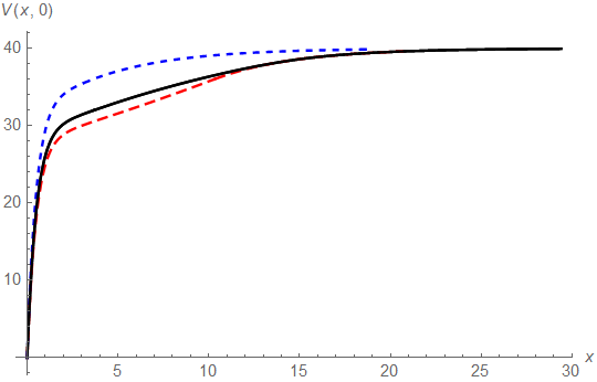
Let us first consider the case (i.e. the maximal allowed dividend rate is the drift of the surplus process ). Figure 1(a) depicts as a function of initial capital together with the value function of the classical dividend problem without ratcheting constraint, for which the optimal strategy is a threshold strategy of not paying any dividends when the surplus level is below and pay dividends at rate above . Recall from Asmussen and Taksar [7] or also Gerber and Shiu [20] that in the notation of the present paper
with optimal threshold
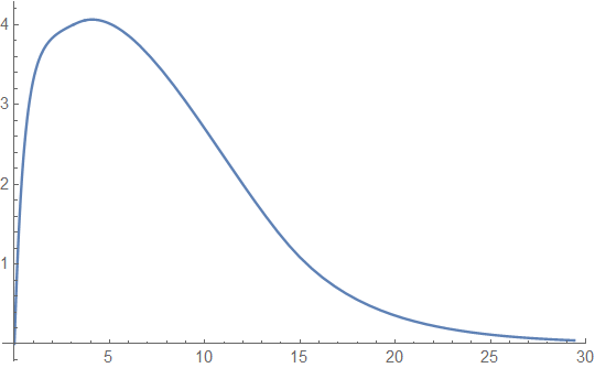
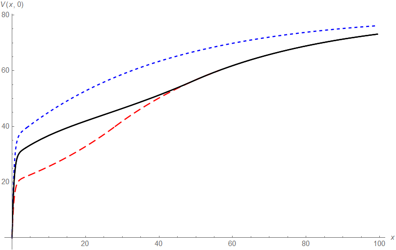
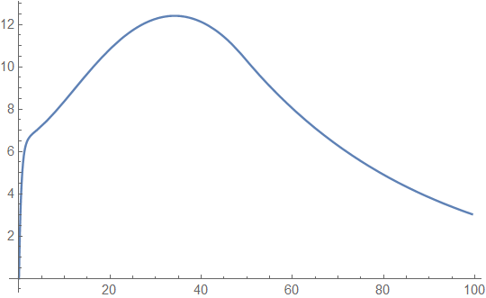
One observes that for both small and large initial capital the efficiency loss when introducing the ratcheting constraint is very small, only for intermediate values of the resulting expected discounted dividends are significantly smaller, but even there the relative efficiency loss is not big (see Figure 2(a) for a plot of this difference). We also compare in Figure 1(a) with the optimal value function
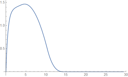
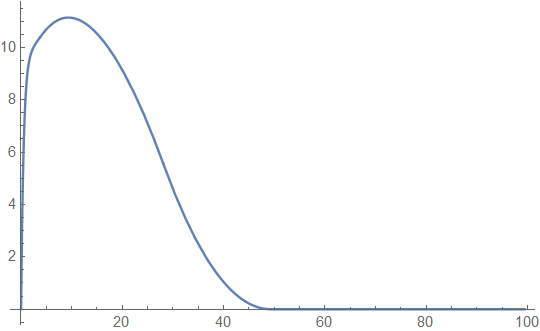
of the further constrained one-step ratcheting strategy, where only once during the lifetime of the process the dividend rate can be increased from 0 to . That latter case was studied in detail in [3], where it was also shown that the optimal threshold level for that switch is exactly the one for which the resulting expected discounted dividends match with the ones of a threshold strategy underlying , but at the (for the latter problem non-optimal) threshold . We observe that the performance of this simple one-step ratcheting is already remarkably close to the one of the overall optimal ratcheting strategy represented by (see also Figure 2(b) for a plot of the difference). A similar effect had already been observed for the optimal ratcheting in the Cramér-Lundberg model (cf. [1]).
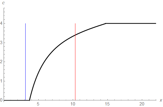
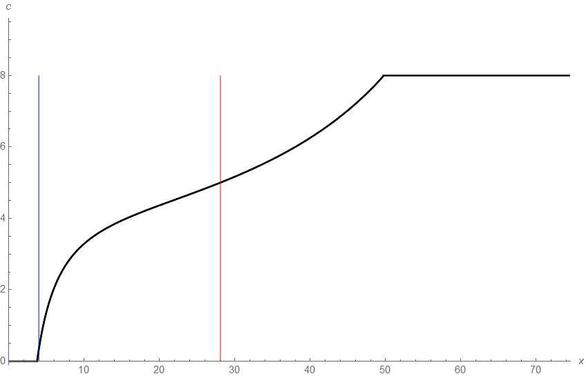
Figure 1(b) depicts the optimal ratcheting curve
underlying for this example together with the optimal threshold
of the unconstrained dividend problem and the optimal switching
barrier for the one-step ratcheting strategy. One sees that the
irreversibility of the dividend rate increase in the ratcheting case leads to
a rather conservative behavior of not starting any (even not small) dividend
payments until the surplus level is above the optimal threshold level
underlying the non-constrained dividend problem. On the other hand,
the one-step ratcheting strategy with optimal switching barrier
roughly in the middle of the optimal curve already leads to a remarkably good
approximation (lower bound) for the performance of the overall optimal
ratcheting strategy.
In Figures 3 and 4 we give the analogous plots for the case , so that the maximal dividend rate is twice as large as the drift of the uncontrolled risk process. The global picture is quite similar, also in this case the efficiency loss introduced by ratcheting is more pronounced and present also for larger initial capital . Also, the further efficiency loss by restricting to a simple one-step ratcheting strategy is considerably larger for not too large . Finally, in that case the first increase of dividends already happens for surplus values (slightly) smaller than the optimal threshold of the unconstrained case.
7 Conclusion
In this paper we studied and solved the problem of finding optimal dividend strategies in a Brownian risk model, when the dividend rate can not be decreased over time. We showed that the value function is the unique viscosity solution of a two-dimensional Hamilton-Jacobi-Bellman equation and it can be approximated arbitrarily closely by threshold strategies for finitely many possible dividend rates, which are established to be optimal in their discrete setting. We used calculus of variation techniques to identify the optimal curve that separates the state space into a change and a non-change region and provided partial results for the overall optimality of this strategy (which can be seen as a two-dimensional analogue of the optimality of dividend threshold strategies in the one-dimensional diffusion setting without the ratcheting constraint). In contrast to [2], the same analysis is applicable for all finite levels of maximal dividend rate , i.e. also if the latter exceeds the drift . We also gave some numerical examples determining the optimal curve strategy. These results illustrate that the ratcheting constraint does not reduce the efficiency of the optimal dividend strategy substantially and that, much as in the compound Poisson setting, the simpler strategy of only stepping up the dividend rate once during the lifetime of the process is surprisingly close to optimal in absolute terms. In terms of a possible direction of future research, as mentioned in Section 5 we conjecture that a curve strategy dividing the state space into a change and a non-change region is optimal in full generality for the diffusion model, and it remains open to formally prove the latter. Furthermore, it could be interesting to extend the results of the present paper to the case where the dividend rate may be decreased by a certain percentage of its current value (see e.g. [5]) or to place the dividend consumption pattern into a general habit formation framework (see e.g. [6] for an interesting related paper in a deterministic setup).
8 Appendix
Let us show now, that there exists such that
| (42) |
for all . Take and such that
| (43) |
the associated control process is given by
Let be the ruin time of the process . Define as and the associated control process
Let be the ruin time of the process ; it holds that for . Hence we have
| (44) |
Let us show now that, given with there exists such that
| (45) |
Take and such that
| (46) |
define the stopping time
| (47) |
and denote the ruin time of the process . Let us consider as ; denote by the associated controlled surplus process and by the corresponding ruin time. We have that and so , which implies
Hence, we can write,
| (48) |
So, we deduce (45), taking We
conclude the result from (41), (42) and (45).
Proof of Proposition 3.1. Let us show first that is a viscosity supersolution in . By Proposition 2.2, in in the viscosity sense.
Consider now and the admissible strategy , which pays dividends at constant rate up to the ruin time . Let be the corresponding controlled surplus process and suppose that there exists a test function for supersolution (8) at . Using Lemma 2.1, we get for
Hence, using Itô’s formula
So, dividing by and taking , we get , so that is a viscosity supersolution at .
Let us prove now that it is a viscosity subsolution in . Assume first that is not a subsolution of (8) at . Then there exist , and a (2,1)-differentiable function with such that ,
| (49) |
for and
| (50) |
for . Consider the controlled risk process corresponding to an admissible strategy and define
Since is non-decreasing and right-continuous, it can be written as
| (51) |
where is a continuous and non-decreasing function.
Take a (2,1)-differentiable function . Using the expression (51) and the change of variables formula (see for instance [24]), we can write
| (52) |
Hence, from (49), we can write
So, from (50)
Hence, using Lemma 2.1, we have that
but this is a contradiction because we have assumed that . So we have the result.
Proof of Lemma 3.2. A locally Lipschitz function is a viscosity supersolution of (8) at , if any test function for supersolution at satisfies
| (53) |
and a locally Lipschitz function is a viscosity subsolution of (8) at if any test function for subsolution at satisfies
| (54) |
Suppose that there is a point such that . Let us define and
for any . We have that is a test function for supersolution of at if and only if is a test function for supersolution of at . We have
| (55) |
and
| (56) |
for Take such that . We define
| (57) |
Since , there exist such that
| (58) |
From (58), we obtain that
| (59) |
Call . Let us consider the set
and, for all , the functions
| (60) |
Calling and , we obtain that , and so
| (61) |
There exists large enough such that if , then , the proof is similar to the one of Lemma 4.5 of [2].
Using the inequality
we obtain that
Since reaches the maximum in in the interior of the set the function
is a test for subsolution for of the HJB equation at the point . In addition, the function
is a test for supersolution for at and so
(because . Hence, , and we have
Assume first that the functions and are (2,1)-differentiable at and respectively. Since defined in (60) reaches a local maximum at , we have that
and so
| (64) |
Defining and , we obtain
It is hence a negative semi-definite matrix, and
In the case that and are not (2,1)-differentiable at and respectively, we can resort to a more general theorem to get a similar result. Using Theorem 3.2 of Crandall, Ishii and Lions [14], it can be proved that for any , there exist real numbers and such that
| (65) |
and
This is a contradiction and so we get the result.
References
- [1] Albrecher, H., Azcue, P. and Muler N. (2017). Optimal dividend strategies for two collaborating insurance companies. Advances in Applied Probability 49, No.2, 515–548.
- [2] Albrecher, H., Azcue, P. and Muler N. (2020), Optimal ratcheting of dividends in insurance. SIAM Journal on Control and Optimization, 58(4), 1822–1845.
- [3] Albrecher H., Bäuerle N. and Bladt M. (2018). Dividends: From refracting to ratcheting. Insurance Math. Econom. 83, 47–58.
- [4] Albrecher, H. and Thonhauser, S. (2009). Optimality results for dividend problems in insurance. RACSAM-Revista de la Real Academia de Ciencias Exactas, Fisicas y Naturales. Serie A. Matematicas 103, No.2, 295–320.
- [5] Angoshtari, B., Bayraktar, E. and Young, V.R. (2019) Optimal dividend distribution under drawdown and ratcheting constraints on dividend rates. SIAM Journal on Financial Mathematics 10, 2, 547–577.
- [6] Angoshtari, B., Bayraktar, E. and Young, V.R. (2020) Optimal Consumption under a Habit-Formation Constraint. arXiv preprint arXiv:2012.02277.
- [7] Asmussen, S.and Taksar, M. (1997). Controlled diffusion models for optimal dividend pay-out. Insurance: Mathematics and Economics 20, 1, 1-15.
- [8] Avanzi, B. (2009). Strategies for dividend distribution: A review. North American Actuarial Journal 13, 2, 217-251.
- [9] Avanzi, B., Tu, V., and Wong, B. (2016). A note on realistic dividends in actuarial surplus models. Risks 4, 4, 37, 1–9.
- [10] Azcue P. and Muler N. (2014). Stochastic Optimization in Insurance: a Dynamic Programming Approach. Springer Briefs in Quantitative Finance. Springer.
- [11] Azcue, P., Muler, N. and Palmowski, Z. (2019). Optimal dividend payments for a two-dimensional insurance risk process. European Actuarial Journal 9, 1, 241–272.
- [12] Bäuerle, N. (2004). Approximation of optimal reinsurance and dividend payout policies. Mathematical Finance, 14, 1, 99–113.
- [13] Cohen, A. and Young, V. R. (2020). Rate of convergence of the probability of ruin in the Cramér-Lundberg model to its diffusion approximation. Insurance: Mathematics and Economics, to appear.
- [14] Crandall, M. G., Ishii, H. and Lions, P. L. (1992). User’s guide to viscosity solutions of second order partial differential equations. Bull. Amer. Math. Soc. (N.S.) 27, 1–67.
- [15] De Finetti, B. (1957). Su un’Impostazione Alternativa della Teoria Collettiva del Rischio. Transactions of the 15th Int. Congress of Actuaries 2, 433–443.
- [16] Dybvig, P.H. (1995). Dusenberry’s ratcheting of consumption: optimal dynamic consumption and investment given intolerance for any decline in standard of living.The Review of Economic Studies, 62, No.2, 287–313.
- [17] Elie, R. and Touzi, N. (2008). Optimal lifetime consumption and investment under a drawdown constraint. Finance and Stochastics 12, 3, 299–330.
- [18] Gerber, H.U. (1969). Entscheidungskriterien fuer den zusammengesetzten Poisson-Prozess. Schweiz. Aktuarver. Mitt. (1969), No.1, 185–227.
- [19] Gerber, H. U. and Shiu, E.S.W. (2004). Optimal dividends: analysis with Brownian motion. North American Actuarial Journal, 8, 1, 1–20.
- [20] Gerber, H. U. and Shiu, E.S.W. (2004). On optimal dividends: from reflection to refraction. Journal of Computational and Applied Mathematics, 186, 1, 4–22.
- [21] Grandits, P. (2019). On the gain of collaboration in a two dimensional ruin problem. European Actuarial Journal 9, 2, 635–644.
- [22] Gu, J., Steffensen, M. and Zheng, H.(2017). Optimal dividend strategies of two collaborating businesses in the diffusion approximation model. Mathematics of Operations Research 43, 2, 377–398.
- [23] Jeon, J., Koo, H.K. and Shin, Y.H. (2018). Portfolio selection with consumption ratcheting. Journal of Economic Dynamics and Control 92, 153–182.
- [24] Protter, P. (1992). Stochastic integration and differential equations. Berlin: Springer Verlag.
- [25] Schmidli, H. (2008). Stochastic Control in Insurance. Springer, New York.