Optimal Online Algorithms for Peak-Demand Reduction Maximization with Energy Storage
Abstract.
The high proportions of demand charges in electric bills motivate large-power customers to leverage energy storage for reducing the peak procurement from the outer grid. Given limited energy storage, we expect to maximize the peak-demand reduction in an online fashion, challenged by the highly uncertain demands and renewable injections, the non-cumulative nature of peak consumption, and the coupling of online decisions. In this paper, we propose an optimal online algorithm that achieves the best competitive ratio, following the idea of maintaining a constant ratio between the online and the optimal offline peak-reduction performance. We further show that the optimal competitive ratio can be computed by solving a linear number of linear-fractional programs. Moreover, we extend the algorithm to adaptively maintain the best competitive ratio given the revealed inputs and actions at each decision-making round. The adaptive algorithm retains the optimal worst-case guarantee and attains improved average-case performance. We evaluate our proposed algorithms using real-world traces and show that they obtain up to peak reduction of the optimal offline benchmark. Additionally, the adaptive algorithm achieves at least more peak reduction against baseline alternatives.
1. Introduction

Electricity bills have been a heavy burden on industrial or commercial consumers (Sun et al., 2010). Typically, commercial buildings spend dollar per square foot per year on electricity (matching the management fee) according to the Commercial Building Energy Consumption Survey (Iota, 2020), while the electricity consumption accounts for up to of the total operating costs of a data center (Rareshide, 2017; Marashi, 2020). The rapid growth of electricity expenses usually relates to higher greenhouse air emissions and goes against sustainable development. Owing to the financial and environmental concerns, these large-load customers have strong desires to study the evolutionary pricing strategies and reduce electricity costs accordingly.
As the introduction of demand side management in the s (Gellings, 1985), utilities tend to exploit delicate pricing schemes for motivating customers to modify their power consumption patterns. As a result of the evolution, a large-power consumer’s electricity bill generally consists of two parts: volume charge and demand charge (Brown, 2017). The volume charge is mainly due to the amount of consumed energy. Moreover, utilities usually adopt time-based rates like Time-of-Use (TOU) pricing (Newsham and Bowker, 2010) to reflect the energy costs over time. However, such pricing strategies may cause rebound peaks, which calls for the second part of the bill (Chakrabortty and Ilić, 2012).
The peak-demand charge refers to the extra punitive charge on the maximum amount of power drawn for any prespecified interval, e.g., or minutes, during a billing period (Brown, 2017). The introduction of peak-demand charge motivates large-power customers to flatten their demand curves. Unlike volume charges (), the peak-demand charge rate is in dollar per kilowatt. According to (CLP Power Hong Kong, 2020), the demand charge rate and on-peak volume charge rate are around HK dollars/kW and HK cents/kWh respectively. It follows that the cost of lifting the peak demand is roughly times that of increasing the off-peak energy consumption by one unit. Moreover, we see that the peak-demand often takes up a large portion of the bill, e.g., up to for DC fast charging stations (Lee et al., 2020) and for Google data centers (Xu and Li, 2014). Therefore, we should pay particular attention to the peak-demand charge.
Two direct approaches to electricity cost saving are reducing peak demands and shifting partial loads from an on-peak period to an off-peak one (Liu et al., 2013; Xu and Li, 2014; Shi et al., 2017). However, such methods are not always applicable, as certain loads cannot be cut or shifted. Meanwhile, bulk energy consumers increasingly invest in self-owned renewable generations, e.g., solar power systems, for green buildings and industries. These installations can reduce the amount of energy purchased from the grid. However, they may result in a more fluctuating net demand curve and not reduce the peak-demand charge because the renewable generations are highly volatile (Jacobsen and Schröder, 2012).
On the other hand, the rapid development of storage technologies makes it convenient and economical to build and maintain a storage system. Energy storage has also been useful to meet demand surges and provide uninterrupted power supply in power systems (Sobieski and Bhavaraju, 1985; Urgaonkar et al., 2011; Guo and Fang, 2013). These facts inspire us to discharge the stored energy in fuel cells or batteries to reduce the peak-demand charge.
As illustrated in Fig. 1, this work targets large-load customers with self-owned renewable generations, and our objective is to maximize the peak-demand reduction by using energy storage in an on-peak period. First note that the volume charge prices are much lower in off-peak periods, so we had better fully charge the storage system then. Second, the on-peak periods of neighbour users often coincide. Thus, recharging may increase the cumulative peak demand in a local grid, which is not socially friendly. Third, energy storage systems, like pumped storage, compressed-air storage, and fuel cells, can not be recharged during use. These facts motivates us to focus on discharging in on-peak periods. Last but not least, our study on storage discharging can shed light on the joint charging/discharging optimization case.
If we know the future demands, it is easier to attain the best use of energy storage. Unfortunately, the small-scale demands are highly uncertain, and self-owned renewable generations even exacerbate the volatility of demands over time (Jacobsen and Schröder, 2012). Consequently, it is challenging to schedule stored energy in real-time to flatten the net demand curves. Furthermore, the non-cumulative nature of peak consumption increases the difficulty in maximizing the peak-demand reduction by using energy storage in an online fashion.
The unpredictability of net demands prevents us from managing stored energy by stochastic optimization or model predictive control. The resulting algorithms may overfit to the estimated model and be sensitive to a volatile practical environment (Urgaonkar et al., 2011; Ma et al., 2012; Alharbi and Bhattacharya, 2017; Qin et al., 2015; Risbeck and Rawlings, 2020). Contrary to these, robust optimization relies little on accurate estimations. It models uncertainties by a set and emphasizes the worst-case outcome of proposed algorithms under the uncertainty set (Bertsimas et al., 2011; Xiang et al., 2015). However, such an approach may suffer from heavy computation and be too conservative.
In our paper, we apply another popular and useful tool, online algorithm design with competitive analysis (Borodin and El-Yaniv, 2005; Buchbinder et al., 2016). In an online setting, an input sequence will be revealed sequentially in time, and the decision maker has to make irrevocable decisions at current time with little or no future information. In our problem, an input sequence refers to a series of demands over time. While stochastic optimization and robust optimization emphasize the absolute performance, competitive online optimization concerns the relative performance compared to the optimal offline outcomes. Specifically, it evaluates an online algorithm via Competitive Ratio (CR), which relates to the worst-case ratio between the offline and online outcomes under the same input sequence. In other words, competitive online optimization considers the robustness by conducting the worst-case analysis and fairness in performance evaluation under different input sequences by adopting the offline-to-online relative performance. More importantly, the best possible CR captures the price of uncertainty for the considered online problem. These merits also indicate the difficulty of applying competitive analysis. To identify the worst-case relative performance and develop online algorithms with the best CR, we frequently encounter nonconvex and combinatorial problems at first sight. Despite these challenges, we shall apply competitive online optimization to the storage-assisted peak-reduction maximization problem under our consideration. We make the following contributions.
In Section 3, we rigorously define the problem as finding an energy storage utilization scheme that maximizes the peak-demand reduction. Moreover, we uncover the inherent structural insights into the optimal offline solution.
In Section 4, we design the first and optimal online algorithm that achieves the best CR. Our algorithm chooses actions to maintain a constant ratio between the online and offline performance at each round. We further show that the best feasible ratio to maintain is also the optimal CR of the problem. Notably, we propose an efficient numerical approach to computing the best CR by a linear number of linear-fractional programs.
In Section 5, we extend our approach to design an adaptive online algorithm that achieves adaptively-improved average-case performance while retaining the worst-case performance guarantee. At each round, the revealed input prunes the uncertainty set and makes it possible to obtain a better CR in the remaining rounds. The adaptive algorithm utilizes the idea and maintains the best possible CR at each round given the revealed input and online actions so far. The adaptive algorithm is among the few online approaches that respond to the non-occurrence of worst-case input and adaptively improve the average-case performance.
In Section 6, we conduct simulations on real-world traces and evaluate the empirical performance of our algorithms in representative scenarios. Simulation results show that our online algorithms improve the peak-demand reduction by more than as compared to baseline alternatives. Further, with little future information, they achieve up to of the (best possible) peak reduction attained by the optimal offline algorithm.
Due to page limitations, omitted proofs can be found in our technical report.
2. Related Work
We discuss three lines of related works in the following.
Using energy storage
As mentioned in the Introduction, more customers exploit energy storage for cost-savings on their electric bills and possible arbitrage opportunities. This phenomenon raises researchers’ interests along this line, as exemplified below. (Walawalkar et al., 2007) assessed the storage value for energy arbitrage and regulation services in New York. (Urgaonkar et al., 2011) explored time-average cost reduction opportunities of using existing storage, like UPS units of data centers. Another kind of existing storage refers to electric vehicles, and the economics of vehicle-to-grid services has been examined in (White and Zhang, 2011). The storage is valuable not only for commercial consumers, but also for residential customers, as discussed in (Leadbetter and Swan, 2012; Ma et al., 2012) and (Xi et al., 2014). In addition to cost-saving, (Jha et al., 2020) investigated reducing emission footprint of the power grid using distributed energy storage. In short, researchers are exploring the applications and potential financial interests of storage from various aspects.
Peak-demand charge
The peak-demand charge has attracted attention from both utilities and large-load customers. (Neufeld, 1987) analyzes the adoption of demand charge given the competition of isolated industrial customers. (Zakeri et al., 2014) considered an extended peak-demand charge which relates to the largest accumulated consumption over several periods. In the literature, researchers have studied multiple approaches for utilities and large-load customers in response to the peak-demand charge. Based on day-ahead load predictions, (Shi et al., 2017) studies the joint optimization of peak shaving and frequency regulation with energy storage. Under a peak-based pricing model, (Zhang et al., 2016) considers the online economic dispatching of local generators in microgrids. (Zhao et al., 2013) and (Lee et al., 2020) respectively examine the scheduling and the pricing of electric vehicle services under the electricity tariff with peak-demand charge. See a survey in (Uddin et al., 2018) for more examples. Overall, the peak-demand charge brings utilities and consumers together for efficient and reliable power systems. In our paper, we consider that a large-load consumer utilizes his or her energy storage to reduce the peak-demand charge. We focus on maximizing the peak-demand reduction brought by using energy storage. Compared with peak-demand minimization that considers the absolute value, the reduction reflects the relative value between the peak-demands before and after using energy storage. It allows us to make a fair comparison on the benefit of the storage under different demand profiles.
Online competitive analysis
Online competitive analysis has been useful in electric vehicle charging (Zhao et al., 2013; Tang et al., 2014; Yi et al., 2019) and economic dispatching (Zhang et al., 2016; Chau et al., 2016). The competitive analyses of cost minimization and benefit maximization have different challenges, as discussed in (Shi et al., 2019) and (Yi et al., 2019). Although we can easily transform the problem from one to the other in the offline scenario, solutions and results for one problem may not directly apply to its counterpart. In this paper, we consider online peak-demand reduction maximization.
We adopt a similar algorithmic framework to that of (Yi et al., 2019) and (Lin et al., 2019) for the proposed online storage management problem. The resulting algorithms are parameterized by a ratio “pursued” in each decision-making round, and we can actively adapt the ratio for real-time information. It turns out that our algorithms are effective and efficient from theoretical analysis and empirical validations.
3. Problem Formulation
In this section, we elaborate on the model of applying energy storage to reduce the peak-demand. We formulate the problem as a peak-demand reduction maximization problem under a capacity constraint and discharging rate constraint. We also introduce the offline optimal solution to the problem given the input is known in advance and emphasize our focus on the practical online scenario. In Table 1, we summarize the useful symbols and terms for future reference.
| Symbols | Meanings |
|---|---|
| scaled storage energy capacity (kWh) | |
| number of time slots | |
| a demand profile, , where is the net demand at time slot (kWh) | |
| lower and upper bounds of the net demand at a time slot (kWh) | |
| discharging quantity at time slot , (kWh) | |
| maximum discharging quantity per time slot (kWh) | |
| peak usage of the offline optimal solution under demand profile | |
| peak-demand reduction of the offline optimal solution under demand profile | |
| solution of pCR-PRM() under demand profile | |
| the best possible CR among all online algorithms | |
| adaptive CR at time slot |
3.1. Mathematical Model
We assume that the peak demand of a large-power customer may occur in time slots of an on-peak period, like from a.m. to p.m. for a shopping mall (Lepage, 2020). Each time slot corresponds to or minutes by the power measurement. Then, we can consider the consumed energy (in kWh) instead of the power demand (in kW).
Net electricity demand:
We consider a general setting where the excess renewable generation cannot recharge the storage system. The self-owned renewable generations are not sufficient to cover the gross demand of the large-load customer during the slots. Then, we use to denote the net demand profile, which is given by the difference between the gross demand and the renewable generation. Although the cost of renewable generation is negligible, the volatile renewable generations exacerbate the unpredictability of net demands over time. Consequently, it is hard to estimate accurately before time slot . We just know the lower and upper bounds of the net demand in a time slot. For brevity, we herein focus on the case with uniform bounds, namely for all ,111In this paper, we use to denote where and reduces to the empty set. while our approach also applies to the case with time-variant bounds after slight modifications.
Energy storage:
Let (in kWh) be the energy storage capacity scaled by a factor concerning the maximum depth of discharge and the discharging efficiency. Let (in kWh) denote the maximum discharging quantity per time slot. In practice, we can hybridize different energy storage technologies with complementary characteristics (Hemmati and Saboori, 2016). For example, flywheel and supercapacity are high power devices, while fuel cells and pumped hydro are high energy devices. In this way, we can attain desired and to meet long-term energy needs and short-term power needs. We consider the scenario that we have fully charged the energy storage before the on-peak period and discharge the storage in the on-peak duration to reduce the peak-demand. We denote the discharging vector by , where (in kWh) is the discharging quantity at time slot . Then, the characteristics of the storage system leads to the inventory constraint and the rate constraints , for all .
3.2. Problem Formulation
To investigate the benefit of implementing energy storage, we formulate and study the following Peak-demand Reduction Maximization (PRM) problem,
| (1) |
The objective represents the peak-demand reduction introduced by the energy storage. If there is no storage, the peak usage under the demand profile is . After applying the discharging vector , we reduce the peak usage to . The discharging vector should satisfy the capacity and discharging rate constraints. Moreover, each discharging quantity should not exceed the demand of the corresponding slot. Our goal is to maximize the peak-demand reduction by using energy storage, which directly leads to cost reductions on the peak-demand charge. Most existing studies consider the peak minimization objective, namely, . In contrast, we adopt the peak-demand reduction maximization objective in PRM, because it makes us focus on the benefit brought by the energy storage. We observe that the two objectives are consistent in the offline setting because their summation remains a known constant under any feasible solution. Notwithstanding, we should differentiate them in the online setting where we lack the information of , let alone when we evaluate online algorithms by competitive ratios. Moreover, in the online setting, we consider the performance guarantee over an uncertainty set of the demand profiles. is non-constant among different demand profiles. Considering a relative peak-reduction value to instead of the absolute peak-demand value provides a more fair performance comparison among different demand profiles. To the best of our knowledge, our work is the first to study the peak-demand reduction maximization by online competitive analysis.
3.3. Optimal Offline Solution
Clearly, when the demand profile is known, we can easily solve the PRM problem by linear programming. Moreover, the following proposition states that the offline optimal solution to PRM presents a particular threshold-based structure.
Proposition 1.
Given a demand profile , there exists with and an optimal solution to PRM is given by
Note that . A useful observation is that the optimal solution to PRM, is also optimal for the peak-demand minimization problem with the same constraints. For notational convenience, we respectively use and to denote the optimal peak usage and the optimal peak-demand reduction after discharging stored energy, namely,
where is the optimal solution to PRM. While solving the offline PRM problem is easy, it is challenging to determine the discharging quantities in real-time without knowing future demands, i.e., in online manner. (Bar-Noy et al., 2008) proposed an optimal competitive online algorithm for the peak minimization, assuming that the original peak usage is known a priori. However, such an assumption is far from practical. In this paper, we consider a more general model where the prior information on the peak usage comprises the lower and upper demand bounds only. Also, we propose, in the next section, an optimal competitive algorithm for the online PRM problem. Overall, our work complements the literature by considering the peak-demand reduction maximization and not assuming to know the exact value of the original peak usage.
4. Online Algorithm
In this section, we shall propose the first competitive online algorithm for PRM. This algorithm is parameterized by the best possible CR among all online algorithms and attains the optimal worst-case relative performance guarantee regarding the offline-to-online ratio of the peak reduction. The best possible CR varies as we change the time-slot number (), the demand bounds ( and ), the storage capacity (), and the maximum discharging limit (). In general, computing the best CR involves hard min-max optimization and we have to resort to dynamic programming which is time-consuming and computationally expensive. Fortunately, as a unique technical contribution, we show that we can obtain the best CR for the online PRM by solving a linear number of linear-fractional programs in parallel. Note that the best possible CR essentially captures the price of uncertainty before we know any inputs, while the price of uncertainty may change as we observe more data and implement actions in past time slots. In practice, we intend to adaptively exploit the real-time information and pursue the updated prices of uncertainty. The particular structure of the proposed algorithm enables us to achieve this purpose and combine efficiency with robustness. We shall elaborate on this extension in the next section.
4.1. Online Setting
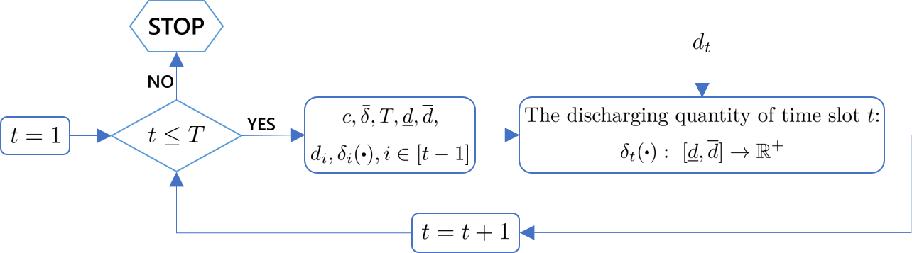
In the online setting, we do not know the exact value of until time slot . The empirical information only tells us that , for all . We denote the set of all possible demand profiles by . Other prior information includes the storage capacity , the maximum discharging limit , and the time-slot number . We present, in Fig. 2, an illustrative flowchart of an online algorithm for PRM.
As mentioned in the introduction, concerning robustness and fairness, CR is a proper measure in online optimization with given resources (Borodin and El-Yaniv, 2005). It quantifies the relative performance between an online algorithm and the offline optimal benchmark. For a maximization problem like PRM, the CR of a deterministic online algorithm is defined as the largest ratio between the objective value under an optimal offline solution and that attained by the algorithm over all possible input sequences (e.g., the demand profiles in PRM), namely,
where refers to the objective values of PRM under the online algorithm and the input sequence . For a randomized algorithm , we can extend the concept of CR by replacing with , where the expectation is due to the random strategies of the algorithm . We always have and a smaller CR indicates that the algorithm can perform more closely to the offline optimal case. We expect to find the online algorithm with the smallest CR, which is the best possible CR among all online algorithms. The best CR not only verifies the optimal performance of the online algorithm, but also quantifies the essential cost of not knowing the future. In other words, the best CR captures the price of uncertainty in the considered online problem.
In the following, we show that it suffices to focus on deterministic online algorithms for the best CR regarding the online PRM.
Proposition 1.
For any randomized algorithm , there exists a deterministic online algorithm such that over all possible input sequence .
4.2. Overview of the CR-Pursuit framework
The usual practice is to propose an online algorithm and then compute its CR for evaluating the performance. In contrast, we herein ask whether there exists an online algorithm with given CR. This question relates to a useful framework for designing competitive online algorithms, called CR-Pursuit. As the name indicates, the CR-Pursuit algorithmic framework requires us to sequentially make online decisions by “pursuing” a prescribed CR. For a maximization problem and a given CR, each CR-Pursuit algorithm will choose actions to maintain an offline-to-online objective ratio to be no more than the CR, in each decision-making round. Despite the conciseness of the idea, there is no general recipe for pursuing the given CR. The means of designing algorithms under CR-Pursuit is problem-specific, as exemplified in (Lin et al., 2019) and (Yi et al., 2019).
We herein summarize several useful observations regarding the CR-Pursuit framework. First, to maintain the offline-to-online ratio in each decision-making round, we usually need to solve an offline problem according to the observed inputs and implemented actions so far. If the offline version of a considered problem is easier, then it is less challenging to design algorithms under CR-Pursuit. Second, the CR-Pursuit framework generally generates a family of algorithms, each of which is characterized by a specific CR. Clearly, the best algorithm among these is the one with the smallest CR. We wonder whether the best algorithm under CR-Pursuit is optimal among all online algorithms. If so, then the CR-Pursuit framework greatly reduces the search space of optimal online algorithms. Overall, there are three main challenges in designing CR-Pursuit algorithms: finding a proper way to sequentially maintain a given CR, identifying the best CR which can be pursued, and checking whether the best CR under CR-Pursuit is the optimal one among all online algorithms. In the following, we shall tackle these challenges with the online PRM. First of all, we shall devise a collection of online algorithms under the CR-Pursuit framework. Then, we show that the best algorithm among these is also optimal among all online algorithms for PRM. Finally, we attain the best online algorithm for PRM by finding the best possible CR.
4.3. Optimal Online Algorithm for PRM
Without knowing future inputs, it seems impossible to maintain the offline-to-online objective ratio to be no more than a given ratio. If we do not know the time-slot number , we can simply assume that there are no future inputs, as has been done in the existing results (Lin et al., 2019; Yi et al., 2019). However, in the online PRM, we are challenged by the facts that is known and the future inputs will affect the online and offline optimal peak-demand reductions. As a result, we shall introduce a reference input and adaptively update it at each time slot . Specifically, we set the reference input sequence at time slot as
Clearly, the reference input sequence is a combination of the observed demands until time slot and the lowest possible future demands, indicating the most optimistic forecast. Given a ratio , we shall apply CR-Pursuit framework and maintain the offline-to-online ratio under the reference input sequence to be more than at each time slot . To this end, we design a family of algorithms, each of which is characterized by a prescribed ratio and called pCR-PRM(). The details of pCR-PRM() are given in Algorithm 1. For notational convenience, we use to denote the output sequence of pCR-PRM() under input sequence .
Alert readers may put forward two issues. First, pCR-PRM() may generate infeasible solutions to PRM. Second, we wonder whether the formula in Algorithm 1 can maintain the offline-to-online objective ratio under to be no more than , for all . For the first issue, we give the following definition in terms of feasibility of pCR-PRM algorithms.
Definition 2.
pCR-PRM() is feasible if, for any , the solution is feasible for PRM.
We address the second issue by the following lemma.
Lemma 3.
Given pCR-PRM(), it holds for any that
Therefore, we conclude that pCR-PRM() can maintain the given CR if and only if it is feasible. Our goal is to find the smallest such that pCR-PRM() is feasible. To this end, we shall first characterize the set of all ratios such that the corresponding pCR-PRM algorithms are feasible. For this purpose, we define an inventory function, which maps a given ratio to the maximum accumulated discharging quantity over all possible demand profiles under pCR-PRM():
We show below that the feasibility of pCR-PRM() is mainly subject to the inventory constraint.
Proposition 4.
pCR-PRM() is feasible if and only if .
The following lemma unravels the monotonicity of the inventory function .
Lemma 5.
is non-increasing and strictly decreases in when .
From Lemma 5, we see that there exists a ratio such that pCR-PRM() is feasible only if . We shall show that pCR-PRM() is the best pCR-PRM algorithm. More importantly, the best pCR-PRM algorithm also attains the optimal CR among all online algorithms for PRM, as stated in the following theorem.
Theorem 6.
Given , , , and , the unique solution to the equation is the best possible competitive ratio among all online algorithms for PRM.
The above theorem indicates that the solution to characterizes the price of uncertainty regarding the online PRM. To find the best online algorithm for PRM, it suffices to search for the best feasible pCR-PRM algorithm. In the next subsection, we shall show an efficient way to find the best possible CR .
4.4. Finding the Optimal Competitive Ratio
Deriving the analytic expression of over all the parameters is attractive but challenging. Instead, we shall explore efficient numerical methods for the best CR . As a unique technical contribution, we show that computing is not much harder than linear programming. Specifically, we first show that the best CR is the maximum of an exponential number of linear-fractional programs. Then, we exploit the problem structure and show that only a linear number of such programs are necessary in terms of the time-slot number . Note that we can transform each involved linear-fractional program into an equivalent linear program by the techniques in (Boyd and Vandenberghe, 2004, Section 4.3.2).
Recall the key formula of pCR-PRM() and the feasibility condition of pCR-PRM(). We conclude that pCR-PRM() is feasible if and only if for any nonempty subset of the index set and any demand profile , it holds that . It follows that
| (2) |
A worst-case input sequence for pCR-PRM() refers to a demand profile , under which the pCR-PRM() algorithm will use up the storage, namely . Since , there exists a worst-case input sequence for pCR-PRM(). Let be a worst-case input sequence and be the set . Then, we observe that the equality in Formula (2) holds under the index set and the input sequence . Therefore, we attain the following proposition.
Proposition 7.
Given , , , and , the best possible CR for the online PRM is given by
Proposition 7 follows directly from Lemma 5 and Proposition 4. Equipped with Proposition 7, we shall transform the computation of the best CR into solving a sequence of linear-fractional programs. Before proceeding, we observe that and the largest element in appears in the first elements. Moreover, we introduce a useful lemma below.
Lemma 8.
Given and , it follows that .
Next, we shall define a family of linear-fractional programs. Each program is parameterized by a nonempty set and its optimal objective value gives a lower bound of the best CR :
Now, let us interpret the variables, constraints and objective of CR-Comp(). are auxiliary variables corresponding to . More specifically, by Lemma 8 and the constraints on the last line, CR-Comp() will attain its optimum when , for all . The remaining constraints of CR-Comp() are associated with the offline PRM problem solved at each time slot under a pCR-PRM algorithm. Precisely, for each , the variable and the variables are respectively related to the optimal objective value and the optimal solution to PRM under the demand profile . CR-Comp() will attain its optimum when , for all . Moreover, the objective function of CR-Comp() corresponds to the left part of Formula (2), noting that . With a slight abuse of notation, we also use to denote the optimal objective value of the linear-fractional program. As a whole, by Lemma 8, Proposition 7, and the above analysis, we attain the following proposition.
Proposition 9.
For each nonempty set ,
Thus, by Proposition 7 and Proposition 9, we conclude that the best possible CR equals . That is to say, we can compute by solving a collection of linear-fractional programs CR-Comp(). Recall that we can convert CR-Comp() into an equivalent linear program. Thus, computing is not much harder than solving a collection of linear programs. Moreover, we can compute these programs in parallel, since none of the programs relies on the solution to another. Nevertheless, a direct application of the above results requires to solve an exponential number of linear programs, which is undesirable. Thus, we are motivated to exploit the structure of pCR-PRM() and exclude as many redundant programs as possible. To this end, we derive the following lemma. It identifies a particular worst-case input sequence for pCR-PRM(), which continuously discharge stored energy until using up the capacity.


Lemma 10.
There exists a worst-case input sequence for pCR-PRM() such that if is greater than a certain index and otherwise.
By Proposition 7, Proposition 9, and Lemma 10, we see that there exists such that . Thus ,we have the following theorem stating that only a linear number () of CR-Comp() programs are necessary for the best possible CR , instead of the exponential number .
Theorem 11.
The best possible competitive ratio for the online PRM is given by
In Fig. 3, we illustrate how the best possible CR varies as each of the parameters changes. We observe that the optimal CR increases as increases and decreases. becomes smaller when and getting closer as it reduces the space of the demand profiles. is non-decreasing in . When is small, e.g., , the best reduction for both online and offline is , and the optimal CR is one.
5. Adaptive pCR-PRM Algorithm
While pCR-PRM() attains the optimal CR among all online algorithms for PRM, it merely focuses on the worst-case performance, which may restrict its performance in practice. We herein extend the pCR-PRM() algorithm by adaptively exploiting the revealed information of previous slots. Here is the intuitive idea: when we realize from the observed inputs that the net demand profile is by no means a worst-case input sequence, we should be more opportunistic and attempt to maintain smaller ratios in the following time slots. In this way, we can improve the average-case performance and still attain the optimal worst-case performance. The underlying reason lies in that the price of future uncertainty changes as we observe more inputs and capturing such variations is critical to the improvement of online decisions. Overall, the results in this section suggest the potential of merging efficiency into robustness.
With respect to the real-time information, we first extend the concept of CR to a time-variant adaptive CR for every online algorithm for PRM at each time slot . Specifically, we make the following definition.
Definition 1.
Given revealed inputs , the adaptive CR at time slot of an online algorithm is defined as
Let be the set of online algorithms whose first outputs are supposing that the first inputs are . Then, considering the observed inputs and implemented actions so far, the best adaptive CR at time slot is given by
Similarly to before, the best adaptive CR at time slot characterizes the price of uncertainty at time slot , for all . Specifically, an online algorithm can at best maintain the online-to-offline ratio of peak-demand reduction to be , for all future inputs. It is clear that is subject to the observed inputs and actions, for all . Based on the introduction of best adaptive CRs, we are ready to introduce the adaptive extension of pCR-PRM.
At each time slot , the adaptive pCR-PRM maintains the online-to-offline ratio of the peak-demand reduction to be no more than the best adaptive CR , instead of a constant CR . We present the pseudocodes of the adaptive pCR-PRM in Algorithm 2.
The remaining issue is on characterizing , the best adaptive CR at each slot. To proceed, we rely on the following observations.
-
•
We observe that the best adaptive CR is no more than the best CR , because we exploit the additional information . Since the adaptive pCR-PRM algorithm makes decisions by pursuing the best adaptive CR at each time slot, we conclude that the sequence is nonincreasing in ,
-
•
Given the online actions before time slot , , the online peak-demand reduction under the demand profile is no more than , Thus, defining
we have .
Based on the observations, we shall show how to search for by a bisection method. To this end, in the following, given observed inputs and made decisions , we define a linear program parameterized by a ratio and a set , where :
The objective function corresponds to the sum of discharging quantities over a set of time slots assuming that we maintain the online-to-offline ratio of peak-demand reduction to be From current time slot to . Similar to CR-Comp(), the constraints of are due to the offline PRM problem solved in each time slot under the adaptive pCR-PRM. By similar arguments for computing the best CR , we conclude that the adaptive CR at time slot should be the smallest ratio in such that does not exceed the remaining inventory . Therefore, we can search for by the bisection method in Algorithm 3. Together with Algorithm 3, we complete the introduction of Algorithm 2 and now summarize the theoretical performance in the following proposition.
Proposition 2.
At each time slot , Algorithm 2 achieves the optimal adaptive competitive ratio among all algorithms in .
If the input sequence is in the worst case regarding pCR-PRM(), then , for all . Otherwise, there is an index such that , for all . From this perspective, we show that the adaptive pCR-PRM also attains the optimal CR among all online algorithms for PRM; moreover, it outperforms pCR-PRM() under general cases.
6. Simulation
In this section, we apply the real-world traces to evaluate the performance of our algorithm under diverse settings. We also compare with conceivable alternatives. The results corroborate our theoretical findings and demonstrate the potentials for practical implementation of our approaches.
6.1. Simulation Setups
In the simulation, we consider a scenario where an EV charging station operator uses its storage to reduce its peak demand in a day. We obtain three-month electricity data from an EV charging station in Shenzhen, China. We divide the time into slots with 15-min length and derive the power demand of the charging station at each slot from the data. We then identify the on-peak duration in a day from the data. In particular, we consider a decision period of slots and set the demand bounds as kWh, which are the minimum and maximum demand of the charging station in this three months, respectively.
6.2. Performance Evaluation
and adaptive pCR-PRM We evaluate the performance of these two algorithms under different storage capacities and show the result in Fig. 4. The capacity rate represents the ratio between the storage capacity and the average daily demand of the charging station in the specified on-peak period. The peak reduction refers to the average peak reduction rate, which is the average ratio between the peak reduction achieved by respective algorithms and the original peak demand. For Fig. 4, we observe that all the algorithms perform better as the capacity increases. The adaptive pCR-PRM attains a higher peak reduction as compared with pCR-PRM, which corroborates our theoretical findings in Sec. 5. While with little feature demand information, our online algorithm adaptive pCR-PRM can achieve of the peak reduction of the offline optimal.
Comparison with Alternatives We mainly compare adaptive pCR-PRM with two catalogs of conceivable alternatives, naive threshold-based algorithms and receding horizon control (RHC) algorithms. We show the results in Fig. 5(a) and Fig. 5(b). In particular, we introduce the alternatives as follows,
-
(1)
THR_half and THR_avg represent the algorithms that discharging to a threshold at each slot until using up the storage. THR_half sets the threshold as , and THR_avg sets the threshold as the average offline optimal peak demand after using the storage.
-
(2)
Eql_Dis equally distributes the energy storage capacity at each slot. Eql_Per discharges at a constant ratio of the demand at each slot until the capacity is running out, and sets the ratio the same as the capacity rate.
-
(3)
RHC algorithms assume a look-ahead window of slots (a quarter of the on-peak duration) in our simulation. At each slot, the RHC algorithms first compute the optimal solution based on the demand in the look-ahead window and their guesses beyond the window. Then, it implements the optimal solution at the current slot and recomputes the optimal at the next slot. RHC_lb, RHC_ub, and RHC_half assume the demand beyond the look-ahead window as , , and , respectively.
From Fig. 5(a), we observe that adaptive pCR-PRM achieves the largest peak-shaving under different capacity rates, with at least improvement against threshold-based algorithms. We observe from the Fig. 5(b) that adaptive pCR-PRM has at least improvement and a relatively small deviation on the peak reduction as compared to the RHC algorithms.


Impact of Discharging Limit We evaluate the performance of adaptive pCR-PRM under different maximum charging rates and compare it with alternatives. The results are shown in Fig. 6. We normalize the discharging rate limit by the upper bound of the demand at a slot. We observe that the adaptive pCR-PRM has close performance under different discharging limits, while the offline optimal achieves greater peak reduction as the discharging limit increases. Without knowing the future demand, adaptive pCR-PRM with a larger charging rate limit may waste more energy at the previously observed peak demand which turns out not to be the peak in the whole period. This prevents adaptive pCR-PRM to obtain higher peak reduction at a larger discharging rate limit. Besides, adaptive pCR-PRM outperforms other alternatives under different charging rate limits.
7. Conclusion
We study an online peak-demand reduction maximization problem under inventory constraints. We focus on a scenario that a large-load power consumer applies energy storage to reduce its peak demand during the on-peak period in a day. We derive an optimal algorithm that achieves the best CR among all online algorithms. We obtain the optimal CR by solving a series of linear-fractional programs. We further extend our algorithm to an adaptive one by exploiting the observed input in real-time. The adaptive pCR-PRM achieves the best adaptive CR at each time slot given the revealed input and online decisions so far. It improves the average-case performance while maintaining the worst-case guarantee. Finally, We evaluate the empirical performance of our algorithms applying real-world traces. We show that the adaptive pCR-PRM achieves close performance to the offline optimal and outperforms the conceivable alternatives. In the future, we shall consider energy storage systems with recharging, e.g., batteries. It is also interesting to extend our techniques for scheduling flexible loads, as in (Zhao et al., 2017).
Acknowledgements.
The work presented in this paper was supported in part by a Start-up Grant (Project No. ) from City University of Hong Kong. Qiulin Lin was with the department of Information Engineering, The Chinese University of Hong Kong, during this work.References
- (1)
- Alharbi and Bhattacharya (2017) Hisham Alharbi and Kankar Bhattacharya. 2017. Stochastic optimal planning of battery energy storage systems for isolated microgrids. IEEE Tran. Sustain. Energy 9 (2017), 211–227.
- Bar-Noy et al. (2008) Amotz Bar-Noy, Matthew P Johnson, and Ou Liu. 2008. Peak shaving through resource buffering. In International workshop on Approximation and Online Algorithms. Springer, 147–159.
- Bertsimas et al. (2011) Dimitris Bertsimas, David B. Brown, and Constantine Caramanis. 2011. Theory and applications of robust optimization. SIAM Rev. 53 (2011), 464–501.
- Borodin and El-Yaniv (2005) Allan Borodin and Ran El-Yaniv. 2005. Online Computation and Competitive Analysis. Cambridge University Press.
- Boyd and Vandenberghe (2004) Stephen Boyd and Lieven Vandenberghe. 2004. Convex Optimization. Cambridge University Press.
- Brown (2017) Gwen Brown. 2017. Making sense of demand charges: What are they and how do they work? https://blog.aurorasolar.com/making-sense-of-demand-charges-what-are-they-and-how-do-they-work
- Buchbinder et al. (2016) Niv Buchbinder, Shahar Chen, Joseph Seffi Naor, and Ohad Shamir. 2016. Unified Algorithms for Online Learning and Competitive Analysis. Math. Oper. Res. 41 (2016), 612–625.
- Chakrabortty and Ilić (2012) Aranya Chakrabortty and Marija D. Ilić. 2012. Control and Optimization Methods for Electric Smart Grids. Springer.
- Chau et al. (2016) Chi-Kin Chau, Guanglin Zhang, and Minghua Chen. 2016. Cost minimizing online algorithms for energy storage management with worst-case guarantee. IEEE Trans. Smart Grid 7 (2016), 2691–2702.
- CLP Power Hong Kong (2020) CLP Power Hong Kong. 2020. Non-residential tariff of CLP. https://www.clp.com.hk/en/customer-service/tariff/business-and-other-customers/non-residential-tariff
- Gellings (1985) Clark W Gellings. 1985. The concept of demand-side management for electric utilities. Proc. IEEE 73 (1985), 1468–1470.
- Guo and Fang (2013) Yuanxiong Guo and Yuguang Fang. 2013. Electricity cost saving strategy in data centers by using energy storage. IEEE Trans. Parallel Distrib. Syst. 24 (2013), 1149–1160.
- Hemmati and Saboori (2016) Reza Hemmati and Hedayat Saboori. 2016. Emergence of hybrid energy storage systems in renewable energy and transport applications – A review. Renew. Sustain. Energy Rev. 65 (2016), 11–23.
- Iota (2020) Iota. 2020. What is the average utility cost per square foot of commercial property? https://www.iotacommunications.com/blog/average-utility-cost-per-square-foot-commercial-property/
- Jacobsen and Schröder (2012) Henrik Klinge Jacobsen and Sascha Thorsten Schröder. 2012. Curtailment of renewable generation: Economic optimality and incentives. Energy Policy 49 (2012), 663–675.
- Jha et al. (2020) Rishikesh Jha, Stephen Lee, Srinivasan Iyengar, Mohammad H. Hajiesmaili, David Irwin, and Prashant Shenoy. 2020. Emission-Aware Energy Storage Scheduling for a Greener Grid. In Proceedings of the Eleventh ACM International Conference on Future Energy Systems (e-Energy ’20). 363–373.
- Leadbetter and Swan (2012) Jason Leadbetter and Lukas Swan. 2012. Battery storage system for residential electricity peak demand shaving. Energ. Buildings 55 (2012), 685–692.
- Lee et al. (2020) Zachary J. Lee, John Z. F. Pang, and Steven H. Low. 2020. Pricing EV charging service with demand charge. Electric Power Systems Research 189 (2020), 106694.
- Lepage (2020) Mathilde Lepage. 2020. Dual day and night tariffs: When do they apply? https://www.energyprice.be/blog/2017/10/23/electricity-off-peak-hours/
- Lin et al. (2019) Qiulin Lin, Hanling Yi, John Pang, Minghua Chen, Adam Wierman, Michael Honig, and Yuanzhang Xiao. 2019. Competitive online optimization under inventory constraints. Proc. SIGMETRICS 3 (2019), 1–28.
- Liu et al. (2013) Zhenhua Liu, Adam Wierman, Yuan Chen, Benjamin Razon, and Niangjun Chen. 2013. Data center demand response: Avoiding the coincident peak via workload shifting and local generation. Perform. Evaluation 70 (2013), 770–791.
- Ma et al. (2012) Jingran Ma, S. Joe Qin, Timothy Salsbury, and Peng Xu. 2012. Demand reduction in building energy systems based on economic model predictive control. Chem. Eng. Sci. 67 (2012), 92–100.
- Marashi (2020) Ali Marashi. 2020. Improving data center power consumption and energy efficiency. https://www.vxchnge.com/blog/growing-energy-demands-of-data-centers
- Neufeld (1987) John L. Neufeld. 1987. Price discrimination and the adoption of the electricity demand charge. J. Econ. Hist. (1987), 693–709.
- Newsham and Bowker (2010) Guy R. Newsham and Brent G. Bowker. 2010. The effect of utility time-varying pricing and load control strategies on residential summer peak electricity use: A review. Energy Policy 38 (2010), 3289–3296.
- Qin et al. (2015) Junjie Qin, Yinlam Chow, Jiyan Yang, and Ram Rajagopal. 2015. Online modified greedy algorithm for storage control under uncertainty. IEEE Trans. Power Syst. 31 (2015), 1729–1743.
- Rareshide (2017) Michael Rareshide. 2017. Power in the data center and its cost across the U.S. https://info.siteselectiongroup.com/blog/power-in-the-data-center-and-its-costs-across-the-united-states
- Risbeck and Rawlings (2020) Michael J. Risbeck and James B. Rawlings. 2020. Economic model predictive control for time-varying cost and peak demand charge optimization. IEEE Trans. Autom. Control 65 (2020), 2957–2968.
- Shi et al. (2019) Ming Shi, Xiaojun Lin, and Lei Jiao. 2019. On the Value of Look-Ahead in Competitive Online Convex Optimization. Proc. ACM Meas. Anal. Comput. Syst. 3, 2, Article 22 (June 2019), 42 pages.
- Shi et al. (2017) Yuanyuan Shi, Bolun Xu, Di Wang, and Baosen Zhang. 2017. Using battery storage for peak shaving and frequency regulation: Joint optimization for superlinear gains. IEEE Trans. Power Syst. 33 (2017), 2882–2894.
- Sobieski and Bhavaraju (1985) D. W. Sobieski and M. P. Bhavaraju. 1985. An economic assessment of battery storage in electric utility systems. IEEE Trans. Power App. Syst 12 (1985), 3453–3459.
- Sun et al. (2010) Yongjun Sun, Shengwei Wang, and Gongsheng Huang. 2010. A demand limiting strategy for maximizing monthly cost savings of commercial buildings. Energ. Buildings 42 (2010), 2219–2230.
- Tang et al. (2014) Wanrong Tang, Suzhi Bi, and Ying Jun Angela Zhang. 2014. Online coordinated charging decision algorithm for electric vehicles without future information. IEEE Trans. Smart Grid 5 (2014), 2810–2824.
- Uddin et al. (2018) Moslem Uddin, Mohd Fakhizan Romlie, Mohd Faris Abdullah, Syahirah Abd Halim, Ab Halim Abu Bakar, and Tan Chia Kwang. 2018. A review on peak load shaving strategies. Renewable and Sustainable Energy Reviews 82 (2018), 3323–3332.
- Urgaonkar et al. (2011) Rahul Urgaonkar, Bhuvan Urgaonkar, Michael J. Neely, and Anand Sivasubramaniam. 2011. Optimal power cost management using stored energy in data centers. In Proc. SIGMETRICS. 221–232.
- Walawalkar et al. (2007) Rahul Walawalkar, Jay Apt, and Rick Mancini. 2007. Economics of electric energy storage for energy arbitrage and regulation in New York. Energy Policy 35 (2007), 2558–2568.
- White and Zhang (2011) Corey D. White and K. Max Zhang. 2011. Using vehicle-to-grid technology for frequency regulation and peak-load reduction. J. Power Sources 196 (2011), 3972–3980.
- Xi et al. (2014) Xiaomin Xi, Ramteen Sioshansi, and Vincenzo Marano. 2014. A stochastic dynamic programming model for co-optimization of distributed energy storage. Energy Syst. 5 (2014), 475–505.
- Xiang et al. (2015) Yue Xiang, Junyong Liu, and Yilu Liu. 2015. Robust energy management of microgrid with uncertain renewable generation and load. IEEE Trans. Smart Grid 7 (2015), 1034–1043.
- Xu and Li (2014) Hong Xu and Baochun Li. 2014. Reducing electricity demand charge for data centers with partial execution. In Proc. ACM e-Energy. 51–61.
- Yi et al. (2019) Hanling Yi, Qiulin Lin, and Minghua Chen. 2019. Balancing cost and dissatisfaction in online EV charging under real-time pricing. In IEEE INFOCOM. 1801–1809.
- Zakeri et al. (2014) Golbon Zakeri, D. Craigie, Andy Philpott, and M. Todd. 2014. Optimization of demand response through peak shaving. 42 (2014), 97–101.
- Zhang et al. (2016) Ying Zhang, Mohammad H. Hajiesmaili, Sinan Cai, Minghua Chen, and Qi Zhu. 2016. Peak-aware online economic dispatching for microgrids. IEEE Trans. Smart Grid 9 (2016), 323–335.
- Zhao et al. (2013) Shizhen Zhao, Xiaojun Lin, and Minghua Chen. 2013. Peak-minimizing online EV charging. In Annual Allerton Conference on Communication, Control, and Computing (Allerton). 46–53.
- Zhao et al. (2017) Shizhen Zhao, Xiaojun Lin, and Minghua Chen. 2017. Robust online algorithms for peak-minimizing EV charging under multistage uncertainty. IEEE Trans. Autom. Control 62 (2017), 5739–5754.
Appendix A Proof of Proposition 1
We rewrite the optimal-solution formula as follows:
The existence of is trivial and the function is nonincreasing in . Let be an optimal solution to PRM satisfying . We first assume that . If , then it follows from that and generates a feasible solution attaining the optimum. Otherwise, if , we have and , implying . Second, we assume that . If , then and generates a feasible solution attaining the optimum. Otherwise, we have and , for all . To summarize, we conclude that an optimal solution is given by the formula in Proposition 1.
Appendix B Proof of Proposition 1
Let be a randomized online algorithm for PRM. Without loss of generality, we assume that is a probability distribution over a set of deterministic online algorithms for PRM: . Then, the expected peak reduction under Algorithm and a demand profile is given by
where is the discharging quantity at time slot under Algorithm and the demand profile .
We devise another deterministic algorithm based on the distribution over the algorithm set . Specifically, the discharging quantity of time slot under Algorithm and the demand profile is given by , for all . Since PRM has linear constraints, it follows that the solution generated by Algorithm is always feasible for all . Moreover, the peak reduction under Algorithm and the input sequence is given by
where the inequality is due to the Jensen’s inequality. Thus, we complete the proof.
Appendix C Proof of Lemma 3
It follows from the formula in Algorithm 1 that
Since and are non-decreasing in , we conclude that
If follows that
Then, we complete the proof.
Appendix D Proof of Proposition 4
The necessary part is obvious and it remains to show the sufficient part. First of all, we show that
where the second inequality follows from and . Then, we show that each solution generated by pCR-PRM() satisfies the discharging limit constraint. Specifically, we have
where the last inequality is due to the feasibility of an offline optimal solution to PRM. Thus, we complete the proof by observing that is a feasible solution if and only if it satisfies the inventory constraint.
Appendix E Proof of Lemma 5
Since is nonincreasing in , we conclude that is nonincreasing. Moreover, if , then there exist and such that and . Note that is strictly decreasing when . It follows that is strictly decreasing when .
Appendix F Proof of Theorem 6
It follows from Lemma 5 that the solution to exists and is unique. Moreover, by Proposition 1, we can prove the theorem by showing that pCR-PRM() is better than any other deterministic online algorithm for PRM. We denote by the output sequence under Algorithm and the input sequence . Since , there exists an input sequence such that . Next, we shall show that Algorithm cannot attain a strictly smaller CR than pCR-PRM().
First of all, we set . If , then we set future inputs by , for all , and show that
where the last equality is due to the facts that and . Thus, we conclude that , for any algorithm which attains a CR no smaller than .
If , then we continue by setting . If , then we find the largest time index such that . Such an index exists, since . Then, under the input sequence , the offline-to-online ratio of peak reduction under remains . As a result, the CR should be no less than . If , then it follows from and that for a certain index . Then, under the input sequence , we have
where the last equality follows from the formula of pCR-PRM(). Thus, we conclude that the CR of Algorithm is strictly larger than .
By the above analysis, we conclude that no other deterministic online algorithm attains a CR strictly smaller than . Moreover, we see that the CR of pCR-PAD() is . Therefore, we complete the proof by further applying Proposition 1.
Appendix G Proof of Lemma 10
The existence of a worst-case input sequence for pCR-PRM() follows from Theorem 6. Considering a worst-case input sequence , we assume that there is an index such that
By Proposition 1, we have . It follows that .
Then, we exchange the order of and in and obtain a new input sequence. We show that
It follows that and . For any index other than and , we also observe that . We summarize the discharging quantities over the time slots and obtain that
It follows that and is also a worst-case input sequence for pCR-PRM(). By applying a sequence of exchanges mentioned above, we can finally attain a worst-case input sequence as described in the theorem, which completes the proof.