Optimal Measurement of Drone Swarm in RSS-based Passive Localization with Region Constraints
Abstract
Passive geolocation by multiple unmanned aerial vehicles (UAVs) covers a wide range of military and civilian applications including rescue, wild life tracking and electronic warfare. The sensor-target geometry is known to significantly affect the localization precision. The existing sensor placement strategies mainly work on the cases without any constraints on the sensors locations. However, UAVs cannot fly/hover simply in arbitrary region due to realistic constraints, such as the geographical limitations, the security issues, and the max flying speed. In this paper, optimal geometrical configurations of UAVs in received signal strength (RSS)-based localization under region constraints are investigated. Employing the D-optimal criteria, i.e., minimizing the determinant of Fisher information matrix (FIM), such optimal problem is formulated. Based on the rigorous algebra and geometrical derivations, optimal and also closed form configurations of UAVs under different flying states are proposed. Finally, the effectiveness and practicality of the proposed configurations are demonstrated by simulation examples.
Index Terms:
Unmanned aerial vehicles (UAV), source localization, Fisher information matrix (FIM), optimal measurement, region constraint.I Introduction
Passive geolocation of radio emitters, is a fundamental problem with a wide range of military and civilian applications [1, 2]. Recent advancements in wireless communication and robotic technologies have made it possible to use unmanned aerial vehicles (UAVs) as aerial sensors for geolocation. Compared to traditional mediums, such as cellular localization and satellite localization, rapid deployment, flexible relocation and high chances of experiencing line-of-sight propagation path have been perceived as promising opportunities to provide difficult services [3]. Due to these distinctive advantages, UAV plays an important role in mobile user localization, rescue, wild life tracking and electronic warfare[4, 5, 6, 7].
Typically, UAVs in the localization task are equipped with wireless communication modules and appropriate sensors. Given some potentially noisy measurements from the sensors, the position of the target is estimated on UAV networks or ground servers. According to the diversity of equipped sensors, the localization approaches can be classified into several types, including time of arrival (TOA) [8, 9], time-difference-of-arrival (TDOA) [10, 11, 12], direction of arrival (DOA) [13, 14] and received signal strength (RSS) [3, 15, 16]. Unlike the time/angle based methods, the RSS-based approach requires less on the signal propagation environment. Moreover, it is cost-effective since it does not require tight synchronization and calibration. In this paper, we consider a passive localization on a ground target using drone swarm equipped with RSS sensors.
Many well-known methods have been proposed in the literature to estimate the location of radio emitters [17, 18, 19]. The best possible accuracy of any unbiased estimator is determined by the Cramer-Rao lower bounds (CRLBs). The CRLB of the UAVs-based localization i.e., the low bound of estimation error variance, contains two ingredients: the inherent configuration and the measurement condition. The measurement condition is related to the signal propagation environment and measuring property of UAVs. Besides, the inherent configuration error is determined by UAV-target (sensor-target) geometry. It turns out that the measuring positions of UAVs significantly affect the estimation precision. Therefore, how to determine the measuring positions of UAVs becomes an important problem.
This kind of measurement configuration problem has attracted much attention in decades. The CRLB matrix and the Fisher information matrix (FIM) are commonly used as the evaluation standards for designing such configurations [20]. Specifically, three optimal criterions have been widely used to help calculate the optimal sensor-target geometries. They are E-optimality criterion (minimizing the maximum eigenvalue of CRLB matrix), D-optimality criterion (maximizing the determinant of FIM) and A-optimality criterion (minimizing the trace of CRLB matrix). There is a rapidly growing research concerned with the optimal RSS sensor-target geometry problem [21, 22, 23, 24]. In [21], authors proposed closed form optimal sensor-target geometry of two and three sensors with inconsistent sensor-target ranges. In [22], the optimal geometries were acquired using a resistor network method in a three-dimension (3D) case. In [23], necessary and sufficient conditions of optimal placements in two-dimension (2D) and 3D were proved using frame theory. It shows that in the equal weight case, optimal geometry of the sensors is just at the verticies of a sided regular polygon, being the number of sensors. In [24], a alternating direction method of multipliers (ADMM) framework was proposed to find the optimal sensors placement. However, these works were all limited to the optimal geometry without deployment region constraints. Note that for UAVs in passive geolocation, region constraints can not be negligible due to such constraints as terrain, security, and flying speed factors.
As to the constrained optimal sensors configuration, related studies have been published recently [25, 26, 27, 28]. In [25], the optimal sensor placement was investigated with some sensors being mobile and some other being stationary. In [26], optimal placement problems of heterogeneous range/bearing/RSS sensors were solved under region constraints. Three deployment regions including a segmental arch, a straight line, and an external closed region are considered dependently. However, no closed-form results were reported for a large number of sensors. Closed form optimal placements of range-based sensors in a connected arbitrarily shaped region were derived in [27]. In [28], circular deployment region constraints and minimum safety distance were considered, closed-form optimal placements were derived for a limited number of AoA sensors.
To the best of our knowledge, there has been no result reported considering dynamic sensors with multiple measurements as well as the region constraints related to the moving speed of sensors. In this paper, drone swarm are employed to localize a ground target using RSS measurements. Due to the geographical limitations and the security issues, minimum flying height and minimum UAV-target horizontal distance are considered. Each UAV is allowed to take multiple measurements below max flying speed. The max speed of UAV are also treated as a constraint. Under these geometrical constraints, optimal configurations of UAVs are investigated. Our main contributions are summarized as follows:
-
1.
The optimal geometrical configuration for drone swarm with multiple measurements in RSS-based geolocation is studied. A special form of the FIM is derived. Combining with practical region constraints expressed mathematically, a FIM-based problem formulation is presented.
-
2.
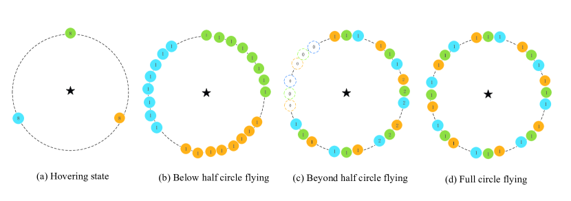
To solve this formulated problem, the optimal UAV-target geometries with fixed flying height and horizontal distance are introduced. After rigorous algebra and geometrical derivations, optimal and also closed form solutions are provided. Altogether, four kinds of optimal configurations are proposed corresponding to the specific flying state of UAVs, including hovering, below half circle flying, beyond half circle flying and full circle flying.
-
3.
Extensive simulations are conducted for various testing scenarios. The simulation results confirm the optimality of proposed configurations. Moreover, a practical scenario is simulated to verify the the practicality of these configurations as well as comparing their robustness.
The rest of the paper is organized as follows. The system model and problem formulation are presented in Section II. In Section III, the optimal configuration with region constraints problem is solved with analytical results for hovering UAVs. In Section IV, the analytical solutions of such problem are derived for flying UAVs with different flying abilities, respectively. Numerical results are presented in Section V, and finally, concluding remarks are given in Section VI.
Notations: Boldface lower case and upper case letters denote vectors and matrices, respectively. Sign denotes the transpose operation and sign denotes the Frobenius norm. Sign represents the trace of a matrix. Sign denotes a Gaussian distribution.
II System Model and Problem Formulation
II-A Measurement Model
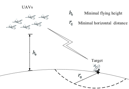
Consider a cooperate localization on a stationary target via UAVs, as illustrated in Fig. 1. The target is located at an unknown position on the ground, denoted as . UAVs search the radio-frequency (RF) signal emitted from the target and measure the RSS.
Each UAV takes multiple measurements while flying or hovering. The measurement amount of the -th UAV is denoted as . The position of the -th UAV at the -th measurement is denoted as . Note that each UAV is aware of its own geographical position using the global positioning system (GPS). Therefore, the distance from this position to the target can be expressed by
| (1) |
According to the well-known radio propagation path loss model (in decibels) [15], the -th measured RSS (in dB) of UAV can be expressed by
| (2) |
where denotes the signal power of the source and denotes the path loss exponent (PLE). It is assumed that the parameters and are known (determined using calibration or prior knowledge) [29, 30, 3]. The measurement noise is denoted as , and .
Based on the measurements, can be inferred using maximum likelihood (ML) estimation. Stacking all measurements of UAV can form a -dimensional column vector, shown as follows.
| (3) |
Accordingly, the probability distribution function (PDF) of the target position is given by
| (4) |
where is the covariance matrix of . As usual, measurement noises among different UAVs are independent. Therefore, the joint PDF based on the whole measurements is given by
| (5) |
II-B Problem Formulation
In this paper, we aim to find optimal geometrical configurations in such localization task. Fisher information matrix (FIM) is well-known to represent the amount of information contained in noisy measurements. Therefore, maximizing the determinant of the FIM, i.e., D-optimality criterion [23, 27, 28], is employed as the optimality metric. Based on the the joint PDF, the FIM can be derived by
| (6) |
Meanwhile, as shown in Fig. 1, a practical condition is considered where UAVs are only able to hover or fly on the limited area while measuring. Due to the safety factor (not detected by the enemy) or geographical limitations, the minimum flying height and the minimum distance to the target must be guaranteed. Corresponding mathematical expressions are given by
| (7a) | |||
| (7b) | |||
Moreover, assume all UAVs have a max flying speed, denoted as . The time interval of two effective measurements is denoted as . This results in the following constraint.
| (8) |
Let and denote the collection of horizontal distances to the target and flying heights, respectively. denotes the collection of horizontal UAV-target angles where . It can be verified that the can be derived from specific , and . To sum up, the mathematical form of this problem is as follows
| (9) |
Remark 1
Note that the objective function in the optimal measurement problem is a function with respect to the real position of the target. Unfortunately, it is unknown, otherwise, the localization task is meaningless. However, in practice, a prior estimation may be available. Therefore, finding the optimal measurement with respect to the prior estimation is useful to refine the estimation. We will discuss this further in the simulation part.
III Optimal Geometrical Configurations of Hovering UAVs
In this section, the optimal solution of problem for hovering UAVs is discussed. The hovering UAVs can be treated as flying UAVs with . In this setting, . First, optimal UAV-target geometries with fixed height and horizontal distance to the target are analysed. Then, the optimal configuration is proposed.
III-A Optimal Geometries with Fixed Height and Horizontal Distance
For the symmetric matrix , we have
| (11) |
Therefore, maximizing the is equal to minimizing the . Using the tight frame theory [31, 32, 33] as introduced in [23], there exists optimal placements minimizing in both regular and irregular cases [23]. Accordingly, optimal geometries are summarized in Theorem 13 and Theorem 2, combining with the focused settings. For convenience, let .
Theorem 1 (Regular optimal geometry)
When (regular case), we have
| (12) |
The equality holds if and only if
| (13) |
Theorem 2 (Irregular optimal geometry)
When (irregular case), we have
| (14) |
The equality holds if and only if
| (15) |
After trivial algebraic operations, the max information amounts in both cases are obtained, given by
| (16) |
| (17) |
III-B Optimal Geometrical Configurations
Due to the split property of the max determinant of FIM, shown in formula (16) and (17), it is straightforward that the optimal horizontal distance and height of UAVs are
| (18a) | |||
| (18b) |
In this configuration, the distance between UAVs to target are all equal to , denoted as . However, this result is only applicable to the special regular or irregular case. To solve problem , further analysis is presented in the following.
For convenience, let . Besides, we define , , , and . Moreover, (16) is simplified as and (17) is simplified as .
Proof: With (18a), (18b) and (13) satisfied, . Obviously, . Therefore, it is optimal in regular cases. Because for any ,, . Therefore, it is optimal compared to any irregular cases. From above, the configuration satisfies (18a), (18b) and (13) is the optimal solution of problem
Proof: With (18a), (18b) and (13) satisfied, . Obviously, . Therefore, the configuration is optimal in irregular cases, and the max determinant of is equal to .
However, there is a candidate in regular cases. Since is an increasing function with respect to and , reaches the max value at an extreme point where and are max in the domain of definition. It is easy to verify that the max and satisfy . It means that except the -th UAV, the other UAV satisfies the boundary conditions of distance and height, while the -th UAV compromises with them to satisfy the regular condition. Therefore, the max determinant of in regular cases is equal to .
At last, comparing the max determinant of in two cases yields
| (19) |
From the above, the configuration satisfies (18a), (18b) and (15) is the optimal solution of problem .
Remark 2
Theorem 3 and Theorem 4 give the optimal configurations for all cases. The optimal distance and height configurations are straightforward. And each UAV performs horizontal circle flying about the target. As for the optimal UAV-target horizontal angles in the regular case, algorithm 1 proposed in [23] can be applied directly to find a closed form solution. In the irregular case, the optimal configuration implies that UAVs from to except are collinear with the target and the line is orthogonal to the line passing through the -th UAV and the target.
IV Optimal Geometrical Configurations for Flying UAVs
In this section, based on the optimal UAV-target geometry in the last section, optimal geometrical configurations for flying UAVs are developed.
IV-A Below Half Circle Flying
Assume each UAV cannot complete a full circle flying with respect to the target during the localization task, i.e., . We consider a special case where and (a regular case).
The FIM in (A) is rewritten as
| (20) |
Note that is just a special form of defined in (10). Therefore, according to Theorem 3, the optimal configuration satisfies (18a), (18b) and (13) with . In this configuration, . It shows that the determinant of FIM is equal to , which is the max value of the objective function in problem .
To satisfy (13) with , the optimal UAV-target horizontal angle configuration at one measurement can be obtained using algorithm 1 proposed in [23]. Let be one of them. According to the principle of equivalent placements [23], rotating the overall angles around the target maintains the optimal property. Mathematically, is also the optimal angle configuration. Considering the flying ability of UAVs, the optimal UAV-target horizontal angle configuration is given by
| (21) |
From the above, the following theorem is proposed.
Remark 3
When (an irregular case), the optimal UAVs-target horizontal angle configuration at one measurement can be obtained using Theorem 2. The proposed UAV-target angle configuration can also be applied directly. However, in this scenario, the proposed configuration may not be optimal, but can be treated as a suboptimal solution of problem .
Remark 4
For , the optimal configuration in hovering state is also a selectable optimal solution. Fig. 2 illustrates both of them. But flying with even a slow speed is more robust considering the prior estimation error in practice. Further discussions are shown in the simulation part.

IV-B Beyond Half Circle or Full Circle Flying
Assume each UAV can complete a full horizontal circle flying with respect to the target during the localization task, i.e., . Let denote the -th UAV-target horizontal angle at the starting position.
The FIM in (A) is rewritten as
| (22) |
Note that is just a special form of defined in (10). Therefore, according to Theorem 3, the optimal configuration satisfies (18a), (18b) for -th UAV. In this way, . The problem belongs to the equally-weighted optimal placements [34, 23]. Accordingly, when , the right angle structure is optimal, given by
| (23) |
When , the uniform angular array (UAA) is optimal, given by
| (24) |
Under this configuration, the determinant of FIM is expressed by
| (25) |
It is easy to verify that in (25) reaches the max value of the objective function in problem (II-B).
Moreover, besides this configuration, their exists other optimal geometrical configurations with beyond half circle flying for . Let denote an arbitrarily integer number satisfying , and . Via flipping some positions in UAA that are measured after the -th measurement about the target, the configuration is completed. Mathematically, in this configuration, we have
| (26) |
According to the principle of equivalent placements [23], this configuration is an equivalent form to the optimal full circle flying configuration, i.e, UAA. Therefore, it is optimal. Fig. 2 illustrates both of them.
Thus, the following theorem is proposed.
Theorem 6
Remark 5
By observing (16), (17) and (25), two conclusions are obtained, summarized as follows. In the regular case, in terms of the max information amount of noisy measurements, flying state is the same as hovering state. In the irregular case, in terms of the max information amount of noisy measurements, flying state is over the hovering state.
Remark 6
For , the optimal configurations with below half circle flying as well as hovering state are also selectable optimal solutions. Fig. 2 illustrates all of them. But a full circle flying is the most robust considering the prior estimation error in practice. Further discussions are shown in the simulation part.
V Simulation
In this section, we provide numerical results to demonstrate the optimal UAV-target geometry as well as the proposed optimal geometrical configurations. Unless noted otherwise, some parameters are set as follows: , , and .
V-A Optimal UAV-Target Geometry
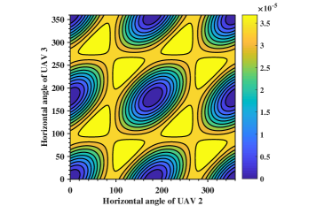
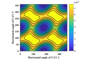
In this subsection, UAVs equipped with RSS sensors are deployed to measure the RF signal from the target while hovering. The horizontal distances to the target and heights satisfy (18a) and (18b) respectively. The -th UAV is hovering with . Both regular and irregular cases are considered. The setting for the regular cases are , named as case (a) and , named as case (b). Meanwhile, the setting for the irregular cases are , named as case (c) and , named as case (d).
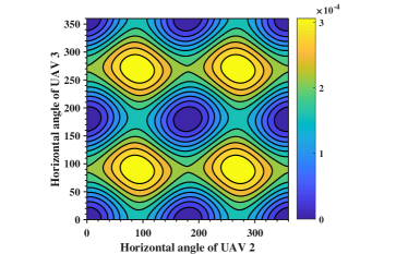
Fig. 3 shows the the FIM determinant via the UAV-target angle configuration. In the regular case (a) (a equally-weighted placement), the optimal angle configurations are , , , , , , , . In the regular case (b), the optimal angle configurations are around , , , . It can be verified that all the optimal configurations are consistent with Theorem 13. In the irregular cases (c) and (d), the optimal angle configurations are , , , . Obviously, the results are the same as Theorem 2.
V-B Optimal Horizontal Distance
In this subsection, UAVs are deployed to measure the RF signal from the target while hovering. Both regular and irregular cases are considered. As for each case, the variance settings maintain the same as the last subsection (case (b) and case (c)). The optimal UAV-target angle configurations are used.
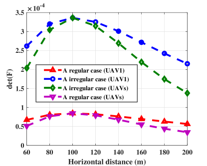
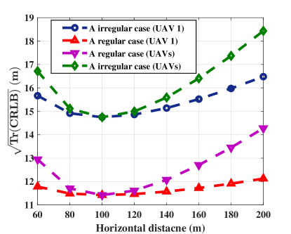
Fig. 4 shows the determinant of FIM and a low bound of root mean square error (RMSE) via hovering horizontal distance to the target. Specifically, the low bound is . When UAV 2 and 3 are fixed, i.e., , the optimal horizontal distance of UAV 1 is equal to . When no UAV is fixed, the optimal horizontal distance of UAVs is also equal to . It is concluded that the optimal UAV-target elevation angle is when . Note that it is different to normal 2D cases where sensors should be be close to the target. The reason is that a additional dimensional exists while measuring the target on the ground via UAVs.
V-C Optimal Configurations with Prior Estimation
In this subsection, a practical scenario is considered where the proposed optimal configurations are used to refine the prior estimation. UAVs are deployed. Among them, the measurement noise variance of ten UAVs are set to be and the others are set to be .
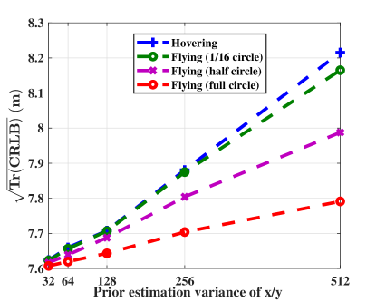
Fig. 5 shows the performances of the proposed configurations via variance of prior estimation error. As observed, the robustness lever is ordered as follows: full circle flying, beyond half circle flying, below half circle flying, hovering. Moreover, the uncertainty of the target has little impact on the proposed configurations, which ensures the practicality of these ideal optimal configurations.
VI Conclusions
In this paper, we have studied the problem of finding the optimal geometrical configuration of drone swarm to localize a ground target. Based on the optimal UAV-target geometry, optimal configurations of UAVs have been proposed for both hovering and flying states with practical region constraints. The numerical results have demonstrated significant benefits of the proposed configurations in both ideal and realistic examples.
Appendix A A form of FIM in Multi-UAVs RSS-based Localization
In this section, a special form of the FIM of the multi-UAVs RSS-based measurements is derived.
Referring to [35], the FIM on the RSS data measured by the -th UAV () can be written as
| (27) |
where
| (28a) | |||
| (28b) | |||
Because measurement noises among different UAVs are assumed to be dependent, (6) can be expressed by
| (29) |
References
- [1] M. Z. Win, Y. Shen, and W. Dai, “A theoretical foundation of network localization and navigation,” Proc. IEEE, vol. 106, no. 7, pp. 1136–1165, 2018.
- [2] M. Chiani, A. Giorgetti, and E. Paolini, “Sensor radar for object tracking,” Proc. IEEE, vol. 106, no. 6, pp. 1022–1041, 2018.
- [3] X. Cheng, W. Shi, W. Cai, W. Zhu, T. Shen, F. Shu, and J. Wang, “Communication-efficient coordinated RSS-based distributed passive localization via drone cluster,” IEEE Trans. Veh. Technol., vol. 71, no. 1, pp. 1072–1076, 2022.
- [4] D.-H. Kim, K. Lee, M.-Y. Park, and J. Lim, “UAV-based localization scheme for battlefield environments,” in Proc IEEE Mil Commun Conf MILCOM, 2013, pp. 562–567.
- [5] Y. Zeng, R. Zhang, and T. J. Lim, “Wireless communications with unmanned aerial vehicles: opportunities and challenges,” IEEE Commun. Mag., vol. 54, no. 5, pp. 36–42, 2016.
- [6] A. Wang, X. Ji, D. Wu, X. Bai, N. Ding, J. Pang, S. Chen, X. Chen, and D. Fang, “GuideLoc: UAV-assisted multitarget localization system for disaster rescue,” Mob. Inf. Sys., vol. 2017, 2017.
- [7] O. M. Cliff, R. Fitch, S. Sukkarieh, D. L. Saunders, and R. Heinsohn, “Online localization of radio-tagged wildlife with an autonomous aerial robot system,” in Robotics: Science and Systems, 2015.
- [8] E. Xu, Z. Ding, and S. Dasgupta, “Source localization in wireless sensor networks from signal Time-of-Arrival measurements,” IEEE Trans. Signal Process., vol. 59, no. 6, pp. 2887–2897, 2011.
- [9] J. Shen, A. F. Molisch, and J. Salmi, “Accurate passive location estimation using TOA measurements,” IEEE Trans. Wireless Commun., vol. 11, no. 6, pp. 2182–2192, 2012.
- [10] K. Ho and Y. Chan, “Solution and performance analysis of geolocation by TDOA,” IEEE Trans. Aerosp. Electron. Syst., vol. 29, no. 4, pp. 1311–1322, 1993.
- [11] F. Shu, S. Yang, Y. Qin, and J. Li, “Approximate analytic quadratic-optimization solution for TDOA-based passive multi-satellite localization with earth constraint,” IEEE Access, vol. 4, pp. 9283–9292, 2016.
- [12] F. Shu, S. Yang, J. Lu, and J. Li, “On impact of earth constraint on TDOA-based localization performance in passive multisatellite localization systems,” IEEE Syst. J., vol. 12, no. 4, pp. 3861–3864, 2018.
- [13] F. Shu, Y. Qin, T. Liu, L. Gui, Y. Zhang, J. Li, and Z. Han, “Low-complexity and high-resolution doa estimation for hybrid analog and digital massive MIMO receive array,” IEEE Trans. Commun., vol. 66, no. 6, pp. 2487–2501, 2018.
- [14] B. Shi, N. Chen, X. Zhu, Y. Qian, Y. Zhang, F. Shu, and J. Wang, “Impact of low-resolution ADC on DOA estimation performance for massive MIMO receive array,” IEEE Syst. J., vol. 16, no. 2, pp. 2635–2638, 2022.
- [15] A. Weiss, “On the accuracy of a cellular location system based on RSS measurements,” IEEE Trans. Veh. Technol., vol. 52, no. 6, pp. 1508–1518, 2003.
- [16] Y. Li, F. Shu, B. Shi, X. Cheng, Y. Song, and J. Wang, “Enhanced RSS-based UAV localization via trajectory and multi-base stations,” IEEE Commun. Lett., vol. 25, no. 6, pp. 1881–1885, 2021.
- [17] T. Zhao and A. Nehorai, “Information-driven distributed maximum likelihood estimation based on gauss-newton method in wireless sensor networks,” IEEE Trans. Signal Process., vol. 55, no. 9, pp. 4669–4682, 2007.
- [18] R. W. Ouyang, A. K.-S. Wong, and C.-T. Lea, “Received signal strength-based wireless localization via semidefinite programming: Noncooperative and cooperative schemes,” IEEE Trans. Veh. Technol., vol. 59, no. 3, pp. 1307–1318, 2010.
- [19] W. Jiang, C. Xu, L. Pei, and W. Yu, “Multidimensional scaling-based TDOA localization scheme using an auxiliary line,” IEEE Signal Process. Lett., vol. 23, no. 4, pp. 546–550, 2016.
- [20] D. Ucinski, Optimal measurement methods for distributed parameter system identification. CRC press, 2004.
- [21] A. N. Bishop and P. Jensfelt, “An optimality analysis of sensor-target geometries for signal strength based localization,” in ISSNIP - Proc. Int. Conf. Intelligent Sens., Sens. Netw. Inf. Process., 2009, pp. 127–132.
- [22] S. Xu, Y. Ou, and W. Zheng, “Optimal sensor-target geometries for 3-D static target localization using received-signal-strength measurements,” IEEE Signal Process. Lett., vol. 26, no. 7, pp. 966–970, 2019.
- [23] S. Zhao, B. M. Chen, and T. H. Lee, “Optimal sensor placement for target localisation and tracking in 2D and 3D,” Int J Control, vol. 86, no. 10, pp. 1687–1704, 2013.
- [24] N. Sahu, L. Wu, P. Babu, B. S. M. R., and B. Ottersten, “Optimal sensor placement for source localization: A unified ADMM approach,” EEE Trans. Veh. Technol., vol. 71, no. 4, pp. 4359–4372, 2022.
- [25] M. Sun and K. Ho, “Optimum sensor placement for fully and partially controllable sensor networks: A unified approach,” Signal process., vol. 102, pp. 58–63, 2014.
- [26] Y. Liang and Y. Jia, “Constrained optimal placements of heterogeneous range/bearing/RSS sensor networks for source localization with distance-dependent noise,” IEEE Geosci. Remote Sens. Lett., vol. 13, no. 11, pp. 1611–1615, 2016.
- [27] M. Sadeghi, F. Behnia, and R. Amiri, “Optimal sensor placement for 2-d range-only target localization in constrained sensor geometry,” IEEE Trans. Signal Process., vol. 68, pp. 2316–2327, 2020.
- [28] X. Fang, J. Li, S. Zhang, W. Chen, and Z. He, “Optimal AOA sensor-source geometry with deployment region constraints,” IEEE Commun. Lett., vol. 26, no. 4, pp. 793–797, 2022.
- [29] S. Tomic, M. Beko, and R. Dinis, “RSS-based localization in wireless sensor networks using convex relaxation: Noncooperative and cooperative schemes,” IEEE Trans. Veh. Technol., vol. 64, no. 5, pp. 2037–2050, 2015.
- [30] A. Coluccia and F. Ricciato, “RSS-based localization via bayesian ranging and iterative least squares positioning,” IEEE Commun. Lett., vol. 18, no. 5, pp. 873–876, 2014.
- [31] J. Kovacevic and A. Chebira, “Life beyond bases: The advent of frames (Part I),” IEEE Signal Process. Mag., vol. 24, no. 4, pp. 86–104, 2007.
- [32] ——, “Life beyond bases: The advent of frames (Part II),” IEEE Signal Process. Mag., vol. 24, no. 5, pp. 115–125, 2007.
- [33] P. G. Casazza, M. Fickus, J. Kovačević, M. T. Leon, and J. C. Tremain, “A physical interpretation of tight frames,” in Harmonic analysis and applications. Springer, 2006, pp. 51–76.
- [34] B. Yang and J. Scheuing, “Cramer-rao bound and optimum sensor array for source localization from time differences of arrival,” in ICASSP IEEE Int Conf Acoust Speech Signal Process Proc, vol. 4, 2005, pp. iv/961–iv/964 Vol. 4.
- [35] S. Xu, Y. Ou, and W. Zheng, “Optimal sensor-target geometries for 3-D static target localization using received-signal-strength measurements,” IEEE Signal Process. Lett., vol. 26, no. 7, pp. 966–970, 2019.