Optimal Linear Filtering for
Discrete-Time Systems with
Infinite-Dimensional Measurements
Abstract
Systems equipped with modern sensing modalities such as vision and lidar gain access to increasingly high-dimensional measurements with which to enact estimation and control schemes. In this article, we examine the continuum limit of high-dimensional measurements and analyze state estimation in linear time-invariant systems with infinite-dimensional measurements but finite-dimensional states, both corrupted by additive noise. We propose a linear filter and derive the corresponding optimal gain functional in the sense of the minimum mean square error, analogous to the classic Kalman filter. By modeling the measurement noise as a wide-sense stationary random field, we are able to derive the optimal linear filter explicitly, in contrast to previous derivations of Kalman filters in distributed-parameter settings. Interestingly, we find that we need only impose conditions that are finite-dimensional in nature to ensure that the filter is asymptotically stable. The proposed filter is verified via simulation of a linearized system with a pinhole camera sensor.
Discrete-Time Linear Systems, Distributed Parameter Systems, Kalman Filtering, State Estimation, Stochastic Fields, Stochastic Processes
1 Introduction
Many systems involve sensors that produce high-dimensional data. These types of systems occur in a wide range of fields, such as modeling economic growth [1], the spiking patterns of neurons in biological systems [2], and vision-based sensing in robotics [3]. In real-time settings with limited computational power, this data is typically converted to a lower-dimensional representation for timely processing, e.g. by extracting a limited number of key features or restricting to a subset of the data.
In this work, we propose to head in the opposite direction, and treat high-dimensional observations as infinite-dimensional random fields on a continuous index set. Our motivation for this approach comes from physics, where it is often more convenient to treat a complex physical system as a continuum, rather than as a large collection of discrete elements. With the right analytical tools, a continuous representation can simplify analysis and offer insights into the behaviour of the underlying high-dimensional system.
A system with infinite-dimensional observations does come with its own challenges however, which require the use of different analytical tools and lead to a new perspective compared to its finite-dimensional counterpart. The characterization of infinite-dimensional measurement noise involves stochastic fields, which must be handled carefully to maintain rigour. An example of this is the need for a generalization of the Fubini-Tonelli theorem to wide-sense stationary random fields, which we will present in Theorem 3.1.
Another important distinction is that in a standard finite-dimensional Kalman filter setup, an optimal gain is given by solving a matrix equation, and existence and uniqueness conditions arise naturally from standard linear algebra results. The infinite-dimensional observation space, however, results in an integral equation. We will show in Section 4 (under certain regularity assumptions) that this can be solved via Fourier methods and that the existence and uniqueness conditions can, surprisingly, still be given by examining properties of finite-dimensional objects. This gives us access to a closed-form continuous representation of the optimal gain, which is amenable to Fourier analysis.
Furthermore, we note that mean square stability of finite-dimensional systems often requires stabilizability and detectability conditions dependent on the state transition matrix, input matrix, and output matrix. For systems with infinite-dimensional measurements, it turns out that for mean square stability of our filter we require (sufficient) notions of stabilizability and detectability that take into account the noise covariance matrix, which is not the case for finite-dimensional systems. This is demonstrated in Section 5.
1.1 Literature Review
Infinite-dimensional representations are widely used in the study of distributed-parameter systems - see e.g. [4, 5, 6]. In such systems, the states and measurements are represented as functions both of time and a continuous-valued index taking values in some domain . The models may be stochastic [7, 8] or deterministic [4], in either discrete or continuous-time [9]. A critical high-level survey of the approaches, claims, and results in this area has been carried out in [5], and a broader treatment of the estimation and control of distributed-parameter systems can be found in [4, 6, 10, 11]. An overview of various observer design methodologies for linear distributed-parameter systems is also given in the survey [12]. Although this survey does not discuss stochastic systems, the references therein are classified as either early lumping models, where the system is discretized before observer design, and late lumping models, where the system is discretized after observer design. In all the works discussed in [12], both the state and measurement spaces are considered infinite-dimensional.
In contrast with the rich body of work above, in this article we examine systems with infinite-dimensional measurements but finite-dimensional states. complementary problem setup occurs in [13], although in that work the system is assumed to have an infinite-dimensional state space and a finite-dimensional measurement space, which sidesteps the issue of calculating the inverse of an infinite-dimensional object, an issue we will discuss further in Section 6.2. The work in [13] uses an orthogonal projection operator to reduce the state to a finite-dimensional subspace and proceeds to establish upper bounds on the resulting discretization error by way of sensitivity analysis of a Ricatti difference equation. A more common approach is the aforementioned early lumping method, where discretization is performed at the start to produce linear models with high-but-finite-dimensional states and measurements. This is the approach taken by [14], where a Kalman filter is designed for a finite-dimensional subset of the infinite-dimensional measurement, corrupted by the additive Gaussian noise that is spatially white. In this article, we do not perform any such lumping, early or late, and our analysis remains firmly in an infinite-dimensional setting.
See Table 1 for a concise summary of early derivations of linear distributed-parameter filters, as well as more recent work. The papers therein employ a number of different approaches, including Green’s function [15], orthogonal projections [7], least squares arguments [16], the Wiener-Hopf method [8], Bayesian approaches [17], and estimation [18], to name a representative handful. The derivation in this article is closest to the orthogonal projection argument given in [7], although here we deal with a discrete-time system. It should also be noted that [7] assumes that the observation noise is both temporally and spatially white, whereas here we do not require the latter property. We do, however, introduce the assumption that the observation noise is stationary, which allows the novel derivation of a closed form expression of the optimal gain in Section 4.3. This form has not been presented in any of these previous works.
The model that we propose is relevant to systems where high-dimensional measurements, for instance from vision, radar, or lidar sensors, are used to estimate a low-dimensional state, such as the position and velocity of an autonomous agent or moving target. To the best of the authors’ knowledge, such systems have not been the focus of previous work in distributed parameter filtering.
1.2 Contributions
Our key contribution is the derivation of an exact solution for the optimal linear filter for discrete-time systems with measurement noise and process noise modeled by random fields and random vectors respectively (Theorem 4.1, Procedure 1). The assumptions of finite state dimension, and that the measurement noise is stationary on domain , enable us to derive the optimal gain functional explicitly in terms of a multi-dimensional Fourier transform on the measurement index set .
This is in contrast to previous works in which the optimal gain is given in terms of a distributed-parameter inverse operator that is either not defined or defined implicitly [8], [17]. Moreover, this inverse can lead to implementation difficulties and is not always guaranteed to exist: these issues are discussed in further detail in Section 6.2. In comparison, our approach allows us to give sufficient conditions for the system to have a well-defined optimal gain function (Section 4): in rough terms, the effective bandwidth of the Fourier transform of the measurement kernel should be smaller than that of the noise covariance kernel.111The term bandwidth here refers to the effective range of “spatial” frequencies present in a measurement, not temporal frequencies.
An advantage of this continuum limit approach is that it enables us to make precise statements about the filters behaviour in the limit when measurement resolution approaches infinity. This paves the way for further analysis, as various finite-point approximation schemes may be formulated and the error compared with the asymptotic error of the optimal infinite-resolution filter in a principled and quantitative manner. Further discussion and analysis of these finite-point approximation schemes will be addressed in future work.
This article contains five significant extensions in comparison to our preliminary work in the conference paper [21].
The first major development is that this work, by way of a Hilbert space framework, presents necessary and sufficient conditions which guarantee the existence and uniqueness of the optimal gain function. Our previous work [21] employed a calculus of variations approach to yield only necessary conditions on the optimal gain function.
The second development is the extension of our proposed algorithm to a -dimensional, not just scalar, measurement domain , allowing much richer sensor data to be modeled without obscuring the underlying spatial correlations. Examples include camera images (), as well as high-resolution lidar and magnetic resonance imaging (MRI) (). This extension entails the use of random fields and Fourier transforms with -dimensional frequency, as opposed to standard random processes and Fourier transforms on a scalar axis. This has also allowed us to present simulation results that involve two-dimensional images, as opposed to the simpler scalar functions previously presented in [21].
The third development is a weakening of the assumptions on the observation noise. The filter provided in [21] was restricted to systems with Gaussian observation noise, whereas the formulation presented here loosens this assumption and instead only requires that the noise be stationary.
The fourth development is that this work clearly defines explicit conditions such that the presented arguments are rigorous, whereas the derivations in [21] were of a more preliminary and exploratory nature. This work provides a list of assumptions such that our derived filter is well-defined, and that each step in the derivation is valid.
The fifth and final development is that we explicitly impose stabilizability and detectability conditions on the system (Section 2.4). The detectability condition in particular involves the measurement noise covariance function, as well as the deterministic dynamical matrix and measurement function. This strongly contrasts with other works in infinite-dimensional systems theory, which impose conditions of strong or weak observability [22, 23] that are agnostic to noise.
These extensions yield a clearer picture of the relationship between the system and the optimal filter, and provide a more generalized solution for the optimal gain.
1.3 Organization
This article is organized as follows. Section 2 outlines the relevant definitions, theorems, and conditions relating to the Hilbert space of random variables and random fields, as well as the multi-dimensional Fourier transform and notions of system stabilizability and detectability. Section 3 gives our model definition and discusses some concrete examples which our model could be feasibly used to represent. This section also summarizes the key assumptions needed to ensure validity of our analysis, and the motivation behind each assumption. Section 4 derives necessary and sufficient conditions for the optimal gain of the proposed filter (4.1), before presenting a unique gain function which satisfies these conditions 4.2. Section 4.3 will present the full filter equations and stability of this filter will be discussed in Section 5. Section 6 will give a procedure to implement this filter, with Section 6.1 discussing computational complexity and Section 6.2 drawing comparisons to existing results. Finally, Section 7 presents a simulated system and analyzes the empirical performance of the filter compared to its expected performance.
2 Preliminaries
2.1 Hilbert Space of Random Variables
In this work, we denote by , the Hilbert space of all real-valued random variables with finite second moments [24, Ch. 20]. The inner product of any two elements is defined by An inner product operating on two random vectors in the Hilbert space of random -vectors is defined by . The derivation used in this article involves defining the state of our observed system as a vector residing in a Hilbert space and then selecting an error-minimizing estimate that resides in a subspace. The following theorem [25, p.51, Th. 2] is fundamental to this approach.
Theorem 2.1 (Hilbert Projection Theorem)
Let be a Hilbert space and a closed subspace of Corresponding to any vector , there exists a unique vector such that Furthermore, a necessary and sufficient condition that is the unique minimizing vector is that
2.2 Random Fields
This article models measurement noise as an additive random field and some care is required when manipulating these objects. Rigorous and extensive analysis of these fields can be found in a number of textbooks [26], [27], [28]. A brief summary of relevant definitions is given below.
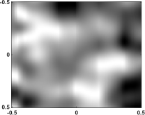
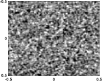
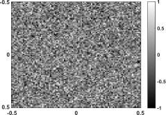
Let be a probability space and a Euclidian space endowed with Lebesgue measure. A random field is a function which is measurable with respect to the product measure on .222For concision, the dependence on will usually be suppressed. A centered w.s.s. (wide-sense stationary) random field has the properties that i) for all ; ii) the random vector for all ; and iii) the covariance function only depends on the difference between index points, so that for any . Such a field that is stationary over a domain is often referred to as stationary noise. In the special case where the covariance is also independent of direction, the noise is said to be isotropic. The stationarity condition arises in situations where the noise statistics possess translational invariance, in other words, the noise statistics look the same everywhere throughout the domain. Some sources of noise may also be locally stationary, in that they are closely approximated by stationary processes over finite windows. Spatial stationarity is a common assumption in a number of diverse contexts such as image denoising [3, 29, 30], radio signal propagation [31], and geostatistics [32, Ch. 74]. Figure 1 gives three example realizations of a stationary random field with a squared exponential covariance function and varying length scales.
2.3 The Multi-Dimensional Fourier Transform
A critical step in this article involves the transformation of an integral equation to an algebraic equation, facilitated by the multi-dimensional Fourier transform, which we now define.
Definition 2.1 (Multi-Dimensional Fourier Transform)
[33, Ch. 1] The multi-dimensional Fourier transform of any is given by and is defined as
where is a -dimensional vector of spatial frequencies. We will denote the Fourier transform of any function by The inverse Fourier transform is defined by
This form of the inverse generally only holds when is also absolutely integrable [34].
2.4 Stabilizability and Detectability
This article will employ notions of stabilizability and detectability, which we define as follows:
Definition 2.2 (Stabilizability)
[35, p. 342] The matrix pair is stabilizable if there exists a matrix such that
where is the spectral radius.
Definition 2.3 (Detectability)
[35, p. 342] The matrix pair is detectable if is stabilizable.
3 Problem Formulation and Assumptions
Consider the linear discrete-time system
| (1) |
with state , additive process noise , state transition matrix , and time index . We omit a control input for clarity; the results derived in this article are still valid with minor changes if a control input is present and available to the estimator. The state is measured via an infinite-dimensional measurement field defined on domain , that is,
| (2) |
Note that the measurement domain , measurement , measurement noise , and measurement function .
The schema presented in (1) and (2) are well-suited to systems where the state can be represented by a low-dimensional model, but the observations are represented by a very high or infinite-dimensional model. A major area where such systems typically hold is robotics, in the context of Simultaneous Localization and Mapping (SLAM). The state to be estimated is often the pose of a mobile robot, which could be described, for example, as a 9-vector that represents the robot position, velocity, and acceleration in . The state updates are generally linear, obeying Newtonian dynamics. The measurement sensors, on the other hand, can be of a much higher dimensionality.
When lighting conditions are adequate, optical cameras provide a rich source of data, and even a relatively cheap 10 megapixel camera will provide a ten million dimensional image every frame. In these conditions, vision-based localization can be particularly suited to GPS-denied areas, such as extra-terrestrial environments [36]. In the case of a colour camera, the measurement equation described (2) would apply with a -vector describing the RGB intensity of each pixel, defined on a dimensional image domain .
Under low or no lighting conditions, where optical cameras do not provide sufficient data, lidar is often employed. This setup has applications in the mining sector [37, 38], where underground tunnels or other ”visually degraded” environments must be traversed [39]. Although not generally as “pixel-dense” as optical cameras, the commonly used SICK LMS511 is capable of providing up to 4560 samples per scan, and higher-end lidar modules can provide upwards of a million samples per scan. This schema is also suited to target-tracking problems, where the state to be estimated now represents a moving body, and the measurement sensors are often radar, lidar, optical, or an ensemble thereof [40].
We assume the additive measurement noise in (2) is a w.s.s. centered random field with bounded covariance function , so that each element of is in for all . We also assume that is bounded and absolutely integrable over domain under the Frobenius or other matrix norm.
The process noise and measurement noise are such that and ,
| (3) | |||||
Here is a positive-definite matrix, is the discrete impulse, and is bounded and absolutely integrable.
We will examine the performance of a linear filter of the form
| (4) |
under a mean square error (MSE) criterion . Here is a linear mapping from the space of -valued fields on to . The innovation term we will denote by . Motivated by the Riesz representation theorem[41, p. 188], we assume the integral form
| (5) |
where is an optimal gain function to be determined.
We now present the assumptions we need, but before we do so, we introduce the following useful terms.
| (6) |
These terms are well-defined given the assumptions below, and we will also show in Section 5 that is symmetric and positive semi-definite, and hence there exists a unique symmetric positive semi-definite matrix such that [42, p. 439]. This matrix will be termed the principal square root of . A summary of the key assumptions stated for our model is now presented.
A1
A2
A3
is invertible for almost all
A4
and has an inverse fourier transform in
A5
A6
The matrix pair is stabilizable.
A7
The matrix pair is detectable.
Assumption A1 and assumption A2 will be used in Section 4.2 to ensure that an appropriate Fourier transform of and is well-defined. Assumption A1 is also needed to extend the Fubini-Tonelli theorem to wide-sense-stationary random fields, as shown in Appendix 9. Assumption A3 and assumption A4 will be needed in Section 4.2 to ensure the existence of an explicit form of the optimal gain function . Assumption A5 is imposed to ensure that the integral (5) is well-defined by Theorem 3.1. Whilst there are notions of observability in infinite-dimensional systems theory (cf. [22, 23]), in this article we do not require them. Instead, we shall assume that is stabilizable (assumption A6) and that is detectable (assumption A7) in the sense of Definition 2.2 and Definition 2.3, where is a matrix-valued functional of the measurement function and the measurement noise covariance . This will ensure that the filter error covariance matrix converges as time grows. It should be noted that traditional detectability conditions do not typically depend on properties of the measurement noise [35, 22, 23].
We verify that the filter integral (5) is well-defined by adapting the classical Fubini-Tonelli theorem [43, Cor. 13.9] to w.s.s. random fields as follows:
Theorem 3.1 (Fubini-Tonelli for w.s.s. random fields)
Let be a w.s.s. random field defined on the probability space , with representing a point in the sample space , and with bounded covariance function . Let be a random field given by , where and is a random vector with elements in and covariance matrix . Also let be a matrix-valued function, absolutely integrable under the Frobenius matrix norm. Each component of the vector-valued function is assumed to be measurable with respect to the product -algebra , where is the -algebra corresponding to the -dimensional Lebesgue measure. Then
4 Optimal Linear Filter Derivation
We wish to find the optimal state estimate , where is some bounded linear functional of all measurements up to time Optimality in this work will refer to the estimate which minimizes the mean square error . This random -vector minimization problem is equivalent to random scalar minimization problems, as minimization of each component norm will minimize the entire vector norm. Each component of is then the orthogonal projection of the corresponding component of onto the space of all scalar-valued linear functionals of the preceding measurements. Let denote the component of the state vector . Also let our observation at time be denoted by the random -vector valued function , assumed measurable with respect to the product measure on , and the set of all possible measurements at time be . Section 4.1 will state the optimality conditions of the filter, and Section 4.2 will derive an explicit solution that satisfies these conditions. A brief reference of the spaces and variables used in the following derivation is given in Table 2 and Table 3 respectively.
| Symbol | Description |
|---|---|
| Hilbert space of random variables with zero mean and finite second moment. | |
| Space of all possible measurements . | |
| Space of all possible elements of expressible via (8). | |
| Space of all possible elements of expressible via (12). | |
| Space of all possible elements of expressible via (10). |
| Symbol | Description |
|---|---|
| System state | |
| Measurement | |
| Optimal estimate of given past measurements | |
| Optimal estimate of given past measurements | |
| Innovation vector | |
| Arbitrary vectors in | |
| Arbitrary element expressible via (8) | |
| Arbitrary element expressible via (10) | |
| Optimal post-measurement correction term | |
| Optimal kernel which generates | |
| The object at time step |
4.1 Optimality Conditions
In this section, we will prove the following key theorem:
Theorem 4.1
The matrix kernel for (4) is optimal in the mean square error sense if and only if
| (7) |
where and denote the posterior covariance matrix and prior covariance matrix of the filter respectively.
Before we provide a proof of Theorem 4.1, we must first define some important sets, and projections onto those sets.
Consider the set of all possible elements of which can be expressed as a bounded linear integral functional operating over all previous measurements:
| (8) | ||||
| . |
Note that is a subspace of . We will also assume for the moment that is a closed subspace of . Suppose that we are already in possession of the optimal estimate of given the previous measurements. This estimate is the orthogonal projection of onto ,
Given the measurements associated with is the best estimate of in the sense that it is the element of that is the unique -norm minimizing vector in relation to the component of the true state.
Let be the element of and denote the orthogonal projection of onto ,
The measurement innovation vector is , the entry of which is denoted Note that for all ,
| (9) |
and let
| (10) | |||
which is a subspace of Here with the row given by .
Lemma 4.2 ()
Given the previous definitions of every element of is orthogonal to every element of
Proof 4.3.
Having shown that the spaces and are orthogonal, we will now find the projection of the true state onto the space of all possible elements in that can be expressed by a bounded linear integral functional operating over all previous measurements and the current measurement. Let be the set of all possible outputs of linear functionals of any element in ,
| (12) | ||||
| . |
Note that using this definition, it immediately follows that , where the addition of sets is given by the Minkowski sum
We also use the operator to refer to a direct sum of subspaces, where any element within the direct sum is uniquely represented by a sum of elements within the relevant subspaces [44]. We wish to find the projection of onto the space of , which is given by
| (13) |
This sum represents a decomposition of the projected state component given measurements up to time as a unique sum of a component within and a component orthogonal to Note that as , it can be formulated as , each being the row, column element of some which must be determined. This matrix-valued function is equivalent to our optimal gain. We are now ready to prove Theorem 4.1, which we will do by formulating necessary and sufficient conditions on the gain such that the optimal post-measurement correction term is generated. The proof of Theorem 4.1 is as follows:
Proof 4.4.
We will denote the column of as By the Hilbert projection theorem, for all , where is guaranteed to be unique. We then have that which, in conjunction with the fact that , implies
| (14) |
This is a necessary and sufficient condition for to be the projection of our state component onto the space We now must find the appropriate optimal gain function such that , the corresponding vector generated, satisfies condition (14) for all Expanding out the definitions of and , interchanging integration and summation, and rearranging, leads to
Note that is simply the vector multiplication The same reasoning may be applied to show We then have for all
Note that as is a random field with bounded covariance function, and is composed of absolutely integrable components, then we may employ Theorem 3.1 and interchange expectation and integration operators. Therefore for all
Because is arbitrary, we must have that for all and almost all
| (15) |
As the first argument is a scalar and the second a vector, the condition that this holds true for all can be conveyed by a single matrix equality. Note that is equivalent to the row of By stacking the row vectors in (15) to form an matrix we may impose the matrix equality that for almost all
| (16) |
Substituting in our value for into (16) we find
Let the posterior covariance matrix be denoted by , and let the prior covariance matrix be denoted by Substituting these terms for the corresponding expectations, we find the optimal gain function must satisfy the condition
Rearranging these terms we arrive at the necessary and sufficient condition
| (17) |
An alternative derivation is given in [21] based on the Calculus of Variations approach. The derivation above, which uses the Hilbert Projection Theorem, has the advantage of a guaranteed uniqueness of the correction term and state estimate , which follows immediately from Theorem 2.1. This approach avoids the use of the functional derivative which has attracted some criticism [8], [5], as well as closely mirroring the methodology of the original Kalman proof [45].
Recall that we initially assumed is a closed subspace. We will now show that an explicit closed-form solution of the optimal gain function can be derived via -dimensional Fourier based methods, thanks to the w.s.s. assumption of the measurement noise. We will then show that when a unique gain function which satisfies (17) exists, it is indeed the case that is closed, which is derived in Corollary 4.5.
4.2 An Explicit Solution for the Optimal Gain Function
We may now proceed to find an explicit value for the optimal gain function that satisfies (7). Consider the matrix-valued functional
| (18) |
and note that,
| (19) |
The left hand side of (19) is simply a multi-dimensional convolution. Many useful properties of the scalar Fourier transform carry over to the multi-dimensional Fourier transform. We will make use of the convolution property [46],
| (20) |
This enables us to find that (19) is equivalent to
| (21) |
Note that will be a vector of the same dimension as . We now require three assumptions to ensure existence and invertibility of the Fourier transform of , as well as the existence of the Fourier transform of : See A1 See A2 See A3 Applying (21) and (20) to (19) implies
| (22) |
For this method to be applicable we must also make the following assumption See A4 Combining (18) and (22) yields
| (23) | ||||
Note that this directly implies that for all , . For simplicity of notation, recall from (6) that Having thus found the optimal function which generates , we now modify (13) to find for any state component ,
These equations may be stacked up into a single matrix equation of the form
| (24) |
where the projection operator acting on the state vector is understood to represent the vector of each components projections. We have thus far assumed that is known to us, we will complete the chain now by determining this value explicitly as
| (25) |
The form of (24) with this substitution is then
where in the last line we substitute , noting that
Finally, we will show that the space is indeed closed, which was previously assumed in Section 4.1. Hence it admits a unique projection by the Hilbert projection theorem (Thm. 2.1), implying the uniqueness of the optimal filter derived above.
Corollary 4.5.
Proof 4.6.
Let us now examine an arbitrary Cauchy sequence with each element in . We also denote . As is a subspace of a closed space , it is guaranteed that exists. For any there exists a unique minimizer such that
As the upper bound goes to zero as increases, and the inequality holds for all , must equal and hence also reside in the space . As the Cauchy sequence was arbitrary, contains all its limit points and is hence closed. It is well known that if two closed linear subspaces of a Hilbert space are orthogonal, then the direct sum of these subspaces is also closed [47, p. 38]. This result, combined with the fact that , implies that if is a closed space, is a closed space for any .
4.3 The Optimal Filter
We now have sufficient knowledge to state a key theorem.
Theorem 4.7.
For the system defined in Section 3, at each time step , the optimal filter gain and associated covariance matrices are given by the equations.
where .
Proof 4.8.
The optimal gain function has been derived in Section 4.2 and is given in (22). It remains to derive the covariance matrix update equations. First, we connect the prior covariance matrix to the covariance matrix of the previous time step, via
| (26) |
Then we determine the relation between and by first observing that expansion and substitution yields the equation
By substitution of (7), all but the first two terms cancel to give us
| (27) |
But this is precisely the equation for defined in (18), so from (23) we simply have
| (28) |
5 Optimal Linear Filter Stability
We will now show that the derived filter provided by Theorem 4.7 is mean square stable under assumptions A1-A7. To do so we will establish via Lemma 5.1 that the associated covariance matrices obey a discrete-time algebraic Riccati equation. We will then, in Theorem 5.3, show that, so long as the initial covariance matrix is non-negative and symmetric, there exists a unique asymptotic a priori covariance matrix that satisfies this Riccati equation.
Lemma 5.1.
Consider the filter equations provided by Theorem 4.7 for the system defined in Section 3. The matrix is positive semi-definite, it is also finite under assumptions A1 and A4. The matrix admits a unique square root decomposition for some symmetric positive semi-definite . Furthermore, for , the a priori covariance matrices satisfy the discrete-time algebraic Riccati equation
| (29) |
Proof 5.2.
First we find that is Hermitian as
where denotes the complex conjugate transpose. is also positive semi-definite, as for almost all and all ,
Define the stationary complex-valued random field . Denote the corresponding auto-covariance function and power spectral density as and respectively. It then follows that
where the last equality is given by the Wiener-Khintchine-Einstein relation [48, p. 82]. As is non-negative, is positive semi-definite for almost all . As is invertible by assumption A3, is positive-definite for almost all . It follows directly that is hermitian and positive-definite for almost all .
It can now be shown that is symmetric and positive semi-definite as
| (30) | ||||
Due to the fact that is Hermitian and is real-valued we then have
The interchange of integral operators in (30) must be justified. This is permitted by the Fubini-Tonelli theorem [43, Cor. 13.9] as each element of is absolutely integrable. This can be seen by noting that every element of is bounded, and that every element of is absolutely integrable, ensuring that every element of is a finite sum of products of absolutely integrable functions and bounded functions and hence is itself absolutely integrable.
This ensures is symmetric. is a hermitian positive-definite matrix and so admits a unique Cholesky decomposition with rank for almost all . We can then state that for almost all ,
hence is positive semi-definite. As is symmetric positive semi-definite, it also admits a unique decomposition for some symmetric positive semi-definite [42, p. 440], proving the first lemma assertion.
Lemma 5.1 is important because it enables us to employ the standard notions of stabilizability and detectability from finite-dimensional linear systems theory to establish the following result characterizing the convergence of our optimal linear filter. Note that Theorem 5.3 requires the following assumptions See A6 See A7
Theorem 5.3.
Consider the filter equations given by Theorem 4.7, and let assumptions A6 and A7 hold. If , then the asymptotic a priori covariance is the unique stabilizing solution of the discrete-time algebraic Riccati equation
Proof 5.4.
Given Lemma 5.1, [35, p. 77] establishes that discrete-time algebraic Riccati equations of the form (29) converge to a unique limit if , is detectable, and is stabilizable. In other words, if these conditions hold, then for any non-negative symmetric initial covariance , there exists a limit
and this limit satisfies the steady-state equation
completing the proof.
Given Theorem 5.3, the asymptotic a posteriori covariance matrix can easily be calculated via the covariance update equation of Theorem 4.7, namely, . Surprisingly, Theorem 5.3 requires only existing concepts from finite-dimensional linear system theory, and no concepts from infinite-dimensional systems theory.
6 Algorithm and Implementation
We will now discuss the computational complexity of Procedure 1 and its connection to existing results, before implementing it in a simulated environment in Section 7.
6.1 Computational Complexity
Our optimal linear filter has many similar properties to the finite-dimensional Kalman filter, such as the convenient ability to calculate the full trajectory of covariance matrices before run-time, as they do not rely on any measurements. This filter is similar to the filter formulated in previous work [21], although the derivation of the filter presented in this work relies on the methodology of projections rather than the calculus of variations approach. The filter given in this article extends the previously derived filter to operate not only on the index set , but on any Euclidian space. Filtering on the Euclidian plane is perhaps the most relevant to imaging applications, but there may be numerous applications involving higher dimensions.
In the standard finite-dimensional Kalman filtering context with measurements, naive inversion of the matrix requires nearly cubic complexity in [49]. This condition can sometimes be ameliorated, however, by observing that if is the covariance matrix of a stationary process then it will have a Toeplitz form. This Toeplitz structure allows greatly reduced computational complexity for inversion operations, see [50] and the references throughout for a brief summary on the types of Toeplitz matrices and corresponding inversion complexities. For positive-definite Toeplitz matrices in particular, inversion may be performed with complexity.
The optimal Kalman filter in Procedure 1 possesses similar advantages due to the stationary structure of . If measurement samples are taken, we see in Procedure 1 that Fourier operations are used to calculate the covariance matrices and optimal gain functions, resulting in a fast Fourier transform applied to an matrix with complexity [51, p. 41].
Although Procedure 1 does contain matrix inversion, this is confined to low-dimensional matrices. This approach to analysis in the continuum provides valuable insights into the optimal gain functions and the behavior of the system. This extension to the continuous measurement domain does introduce a trade-off between accuracy and speed of computation, as any implementable estimator will not be able to sample continuously over the entire space. A standard implementation may sample the space uniformly, which is the approach we take in Section 7, but a more sophisticated approach could involve the analysis of different non-uniform schemes that exploit the underlying system structure. Examination of this trade-off for various systems is an important area of future work.
6.2 Comparisons to Existing Results
During our analysis, we found the necessary and sufficient conditions on the optimal gain satisfies equation (17). If the measurements were finite-dimensional, this equation reduces to a matrix equation. The gain may then be calculated via matrix inversion as
Note that this is the standard equation for the Kalman filter in the finite-dimensional case.
Previous works in this area have also derived condition (17) [19], [16], [8]. These works, however, have either only defined the optimal gain implicitly, or defined it via an operator inverse which satisfies
where is the Dirac delta function [8, Eq. (14)]. The optimal gain is then expressed using this distributed-parameter matrix inverse as
Some derivations also give results where the gain is reliant on These expressions make the connection to the finite-dimensional Kalman filter clearer, but unfortunately the operator inverse is not guaranteed to exist. Furthermore, some forms of will lead to inverses that are troublesome to implement. The derivation of the inverse corresponding to an Ornstein-Uhlenbeck process has been presented previously in [21] and results in an defined in terms of the Dirac delta function and its derivatives. The Dirac delta function is well-defined only when under an integral, and requires special care when implemented on real-world hardware. Derivatives of the Dirac delta function will also cause difficulties in implementation. The filter equations derived in this work do not rely on such an inverse, and give an explicit definition of the optimal gain. The formulation presented will, in some cases, avoid the need for generalized functions such as the aforementioned Dirac delta function and its higher derivatives.
The derived prior covariance update equation (29) can be compared with standard forms for the finite-dimensional Kalman filter [35, p. 39, Eq. (1.9)]. It is interesting to note that this implies that the prior covariance matrix for our filter is equivalent to that of a finite-dimensional Kalman filter with the measurement noise being a standard multi-variate normal distribution and an observation matrix equal to .
We also highlight that the state estimation error previously defined as satisfies
where , and Hence, the state estimation error dynamics and the optimal (component) gains to apply to points in the measurement domain depend on the state dynamics of the system, . In particular, as , the steady-state gain operator must be chosen such that is stable and yields bounded mean square estimation errors. In other words, the gain must take account of the underlying dynamics. This aspect of the filter is important as many standard methods of processing high-dimensional measurements, such as vision-based systems, perform the detection and weighting of measurement features separately from the system dynamics.
7 Simulation Results
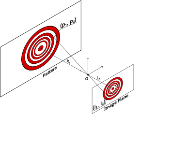
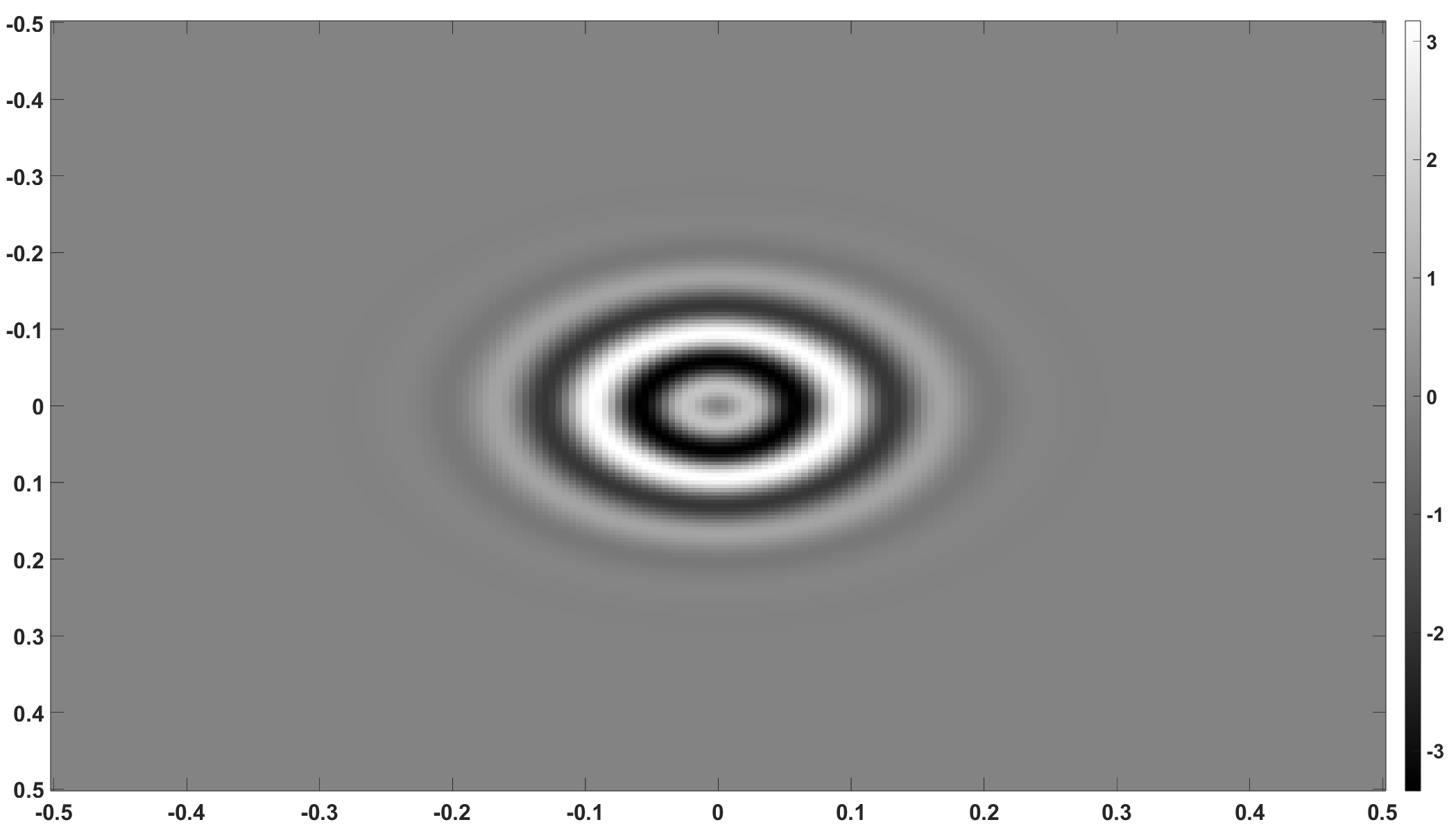
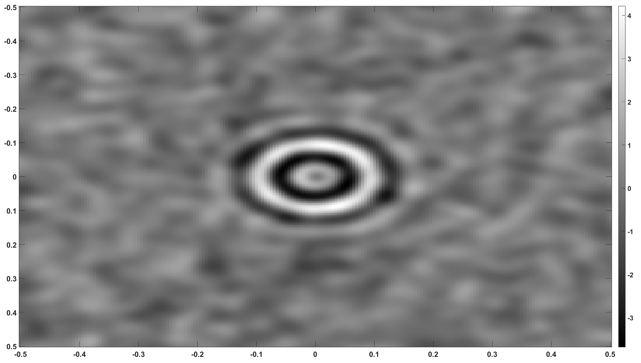
This section presents simulation results for the derived Kalman filter with infinite-dimensional measurements, as described in Algorithm 1. This system consists of a state vector , which represents the position and velocity of some agent. The motion model consists of a state transition model where is the change in time between each discrete step. A two-dimensional image is fixed perpendicular to the line of motion of the filter. This image is represented by the function . We note that the measurement readings are scalar valued, perhaps representing visual light intensity, but this could easily be extended to multi-dimensional image outputs. For example, the intensity of three distinct RGB channels could be represented solely by changing the form of the function to be vector-valued. The measurement model used is the simple pinhole camera model. An illustration of this model is given in Fig. 2. Both the motion model and the measurement model are affected by zero-mean, stationary, additive Gaussian noise such that and
The patterned wall possesses a gray-scale intensity function
| System Variable | Notation | Value |
|---|---|---|
| State Matrix | ||
| Process Noise Covariance | ||
| Measurement Kernel | ||
| State Vector | ||
| Initial State | ||
| Linearization Point | ||
| Integral Domain | ||
| Wall Pattern | ||
| Measurement Covariance | ||
| Initial Error Covariance | ||
| Initial State Estimate | ||
| Time Interval | ||
| Position Variance | ||
| Velocity Variance | ||
| Decay Parameter | ||
| Frequency Parameter | ||
| Measurement Noise Intensity | ||
| Focal Length | ||
| Length Scale | ||
| Sample Spacing |
where is a scalar parameter that determines the decay rate and is a scalar parameter that determines the frequency. Utilizing the pinhole camera model, our non-linear measurement equation is then of the form
This function is linearized around some equilibrium point to derive the linear form used in the simulation. This linearization is given in equation (33) and leads to the corresponding measurement function
| (32) |
The system equations then are:
| (33) |
An example of the linearized measurement pattern as measured by the system without and with noise are presented in Figs. 3(a) and 3(b) respectively.
We can formulate a discrete-time Riccati equation for this system as given by (29).
The matrix pair is stabilizable in the sense of Definition 2.2 because considering a matrix , it is then clear that
It is also true that the matrix pair is detectable in the sense of Definition 2.3, where . This can be shown by demonstrating that the matrix pair is stabilizable, specifically, in the simulated system the matrix takes the form
Considering a matrix of the form
immediately gives that
These conditions, along with the fact that is positive-definite, ensure that the discrete-time Riccati equation for this system possesses a unique stabilizing solution [35]. Utilizing the Matlab function idare and substituting the appropriate terms, the following covariance matrices were calculated for this system.
| (34) |
The process noise of the position and velocity are uncorrelated. A centred, stationary, stochastic field is used to represent the measurement noise, the covariance function of which is a squared exponential also given in table 4.
With the parameters given in Table 4, Algorithm 1 was implemented and simulated using Matlab. It is necessary during implementation to discretise the system appropriately for numerical computation. Numerical functions were evaluated with spacings equal to in each dimension, or a frequency of samples per unit of in each dimension. Algorithm 1 requires numerical integration for the posterior state update step, and the trapz function was used to implement this numerical integration. For this numerical integration step, a finite pixel domain was used. This is larger than the effective pixel-width of and much larger than the effective width of the noise covariance , suggesting minimal impact on the results obtained.
This naive method of numerical integration does not exploit the structure of and hence there may be more efficient numerical methods that do exploit this structure and lead to more efficient computation. Analysis of such techniques and their impact on efficiency will continue to be an important question for future work in this area.
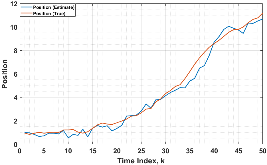
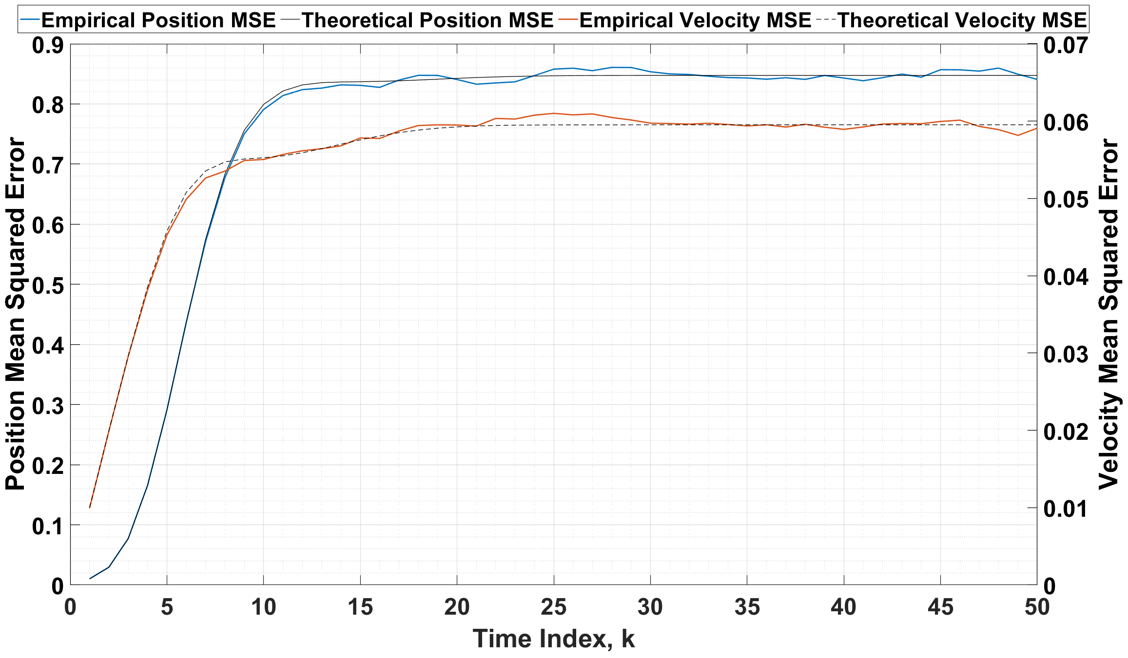
A single realization of the systems true state and the filter estimate over time steps is given in Fig. 4(a). The system was subject to simulated trials and the average MSE of both the position and velocity trajectories calculated. Fig. 4(b) presents these results alongside the theoretical mean square errors according to (34).
8 Conclusion
This article has presented a Kalman filter for a linear system with finite-dimensional states and infinite-dimensional measurements, both corrupted by additive random noise. The assumption that the measurement noise covariance function is stationary allows a closed-form expression of the optimal gain function, whereas previous derivations rely on an implicitly defined inverse. Conditions are derived which ensure the filter is asymptotically stable and, surprisingly, these conditions apply to finite-dimensional components of the system. An algorithm is presented which takes advantage of this stationarity property to reduce computational complexity, and the derived filter is tested in a simulated environment motivated by a linearization of the pinhole camera model.
An extension to a continuous-time framework is possible, but would require additional tools and some further technical conditions, such as the use of stochastic integrals (either in the Itô or Stratonovich sense). An extension of the Fubini-Tonelli theorem given by Theorem 3.1 would also need to be modified to validate the interchange of expectation and integration on stochastic fields over a continuous spatial and temporal field.
Future work includes investigating more efficient means of executing this algorithm, such as non-uniform integration intervals, to yield insight into effective sensor placement. This could be thought of as a form of feature selection, and this principled approach to feature selection may provide insights related to existing heuristics-based and data driven feature selection strategies often employed in high-dimensional measurement processing. It should also be noted that most real-world applications possess non-linear measurement equations and adapting the linear filter to nonlinear systems will be an important area for future work.
9 Existence of Integral (5) via Fubini-Tonelli Theorem
We introduce one final technical assumption:
A8
is measurable with respect to the product -algebra on .
Proof 9.1.
For any fixed , Jensen’s inequality tells us
This implies, due to the non-negativity of norms, that
As this is true for any given , we have the inequality
As is bounded and is absolutely integrable, the first term of the right hand side is finite. By Hölder’s inequality and assumptions A1 and A5 we have and hence the second term as well as the the left hand side is finite. As all norms on are equivalent, we have
where is the element of the vector . As the integral of the absolute expectation of each component is finite, we may apply the Fubini-Tonelli theorem component-wise for each and compose the vector form
References
- [1] A. Belloni and V. Chernozhukov, High Dimensional Sparse Econometric Models: An Introduction, pp. 121–156. Berlin, Heidelberg: Springer Berlin Heidelberg, 2011.
- [2] R. Sepulchre, “Spiking control systems,” Proceedings of the IEEE, vol. 110, no. 5, pp. 577–589, 2022.
- [3] P. Corke, Robotics, Vision and Control - Fundamental Algorithms in MATLAB®, vol. 73 of Springer Tracts in Advanced Robotics. Springer, 2011.
- [4] K. Morris, Controller Design for Distributed Parameter Systems. Springer, 2020.
- [5] R. Curtain, “A survey of infinite-dimensional filtering,” SIAM Review, vol. 17, no. 3, pp. 395–411, 1975.
- [6] A. Bensoussan, G. Da Prato, M. Delfour, and S. Mitter, Representation and Control of Infinite Dimensional Systems. Systems and Control: Foundations and Applications, Birkhauser, 2 ed., 2007.
- [7] S. Tzafestas and J. Nightingale, “Optimal filtering, smoothing and prediction in linear distributed-parameter systems,” Proceedings of the Institution of Electrical Engineers, vol. 115, pp. 1207–1212(5), 1968.
- [8] H. Nagamine, S. Omatu, and T. Soeda, “The optimal filtering problem for a discrete-time distributed parameter system,” International Journal of Systems Science, vol. 10, no. 7, pp. 735–749, 1979.
- [9] P. L. Falb, “Infinite-dimensional filtering: The kalman-bucy filter in hilbert space,” Information and Control, vol. 11, pp. 102–137, 1967.
- [10] Z. Emirsajłow, Output Observers for Linear Infinite-Dimensional Control Systems, pp. 67–92. Cham: Springer International Publishing, 2021.
- [11] R. Curtain and H. Zwart, Introduction to Infinite-Dimensional Systems Theory: A State-Space Approach, vol. 71 of Texts in Applied Mathematics book series. Germany: Springer, 2020.
- [12] Z. Hidayat, R. Babuska, B. De Schutter, and A. Núñez, “Observers for linear distributed-parameter systems: A survey,” in IEEE International Symposium on Robotic and Sensors Environments, pp. 166–171, 2011.
- [13] A. Aalto, “Spatial discretization error in Kalman filtering for discrete-time infinite dimensional systems,” IMA Journal of Mathematical Control and Information, vol. 35, pp. i51–i72, 04 2017.
- [14] A. Küper and S. Waldherr, “Numerical gaussian process kalman filtering for spatiotemporal systems,” IEEE Transactions on Automatic Control, pp. 1–8, 2022.
- [15] F. E. Thau, “On Optimum Filtering for a Class of Linear Distributed-Parameter Systems,” Journal of Basic Engineering, vol. 91, no. 2, pp. 173–178, 1969.
- [16] S. G. Tzafestas, “On the distributed parameter least-squares state estimation theory,” International Journal of Systems Science, vol. 4, no. 6, pp. 833–858, 1973.
- [17] S. G. Tzafestas, “Bayesian approach to distributed-parameter filtering and smoothing,” International Journal of Control, vol. 15, no. 2, pp. 273–295, 1972.
- [18] K. A. Morris, “Optimal output estimation for infinite-dimensional systems with disturbances,” Systems & Control Letters, vol. 146, p. 104803, 2020.
- [19] J. S. Meditch, “Least-squares filtering and smoothing for linear distributed parameter systems,” Automatica, vol. 7, p. 315–322, May 1971.
- [20] A. Bensoussan, Some Remarks on Linear Filtering Theory for Infinite Dimensional Systems, vol. 286, pp. 27–39. Springer Berlin Heidelberg, 10 2003.
- [21] M. M. Varley, T. L. Molloy, and G. N. Nair, “Kalman filtering for discrete-time linear systems with infinite-dimensional observations,” in 2022 American Control Conference (ACC), pp. 296–303, 2022.
- [22] P. A. Fuhrmann, “On observability and stability in infinite-dimensional linear systems,” Journal of Optimization Theory and Applications, vol. 12, pp. 173–181, Aug 1973.
- [23] M. Megan, “Stability and observability for linear discrete-time systems in hilbert spaces,” Bulletin mathématique de la Société des Sciences Mathématiques de la République Socialiste de Roumanie, vol. 24 (72), no. 3, pp. 277–284, 1980.
- [24] B. Fristedt and L. Gray, A Modern Approach to Probability Theory. Boston, MA: Birkhauser, 1997.
- [25] D. G. Luenberger, Optimization by Vector Space Methods. USA: John Wiley & Sons, Inc., 1st ed., 1997.
- [26] R. J. Adler, The Geometry of Random Fields (Probability & Mathematical Statistics S.). John Wiley & Sons Inc, June 1981.
- [27] J. Doob, Stochastic Processes. Probability and Statistics Series, Wiley, 1953.
- [28] S. Janson, Gaussian Hilbert Spaces. Cambridge Tracts in Mathematics, Cambridge University Press, 1997.
- [29] R. Boie and I. Cox, “An analysis of camera noise,” IEEE Transactions on Pattern Analysis and Machine Intelligence, vol. 14, no. 6, pp. 671–674, 1992.
- [30] J. Fehrenbach, P. Weiss, and C. Lorenzo, “Variational algorithms to remove stationary noise: Applications to microscopy imaging,” IEEE Transactions on Image Processing, vol. 21, no. 10, pp. 4420–4430, 2012.
- [31] T. L. Marzetta, “Spatially-stationary propagating random field model for massive mimo small-scale fading,” in 2018 IEEE International Symposium on Information Theory (ISIT), pp. 391–395, 2018.
- [32] P. M. Atkinson and C. D. Lloyd, Geostatistical Models and Spatial Interpolation, pp. 1461–1476. Berlin, Heidelberg: Springer Berlin Heidelberg, 2014.
- [33] E. M. Stein and G. Weiss, Introduction to Fourier Analysis on Euclidean Spaces. Princeton University Press, 1971.
- [34] G. Folland, Fourier Analysis and Its Applications. American Mathematical Society, 2009.
- [35] B. D. O. Anderson and J. B. Moore, Optimal filtering. Prentice-Hall Englewood Cliffs, N.J, 1979.
- [36] A. I. Mourikis, N. Trawny, S. I. Roumeliotis, A. E. Johnson, A. Ansar, and L. Matthies, “Vision-aided inertial navigation for spacecraft entry, descent, and landing,” IEEE Transactions on Robotics, vol. 25, no. 2, pp. 264–280, 2009.
- [37] M. Mascaró, I. Parra-Tsunekawa, C. Tampier, and J. Ruiz-del Solar, “Topological navigation and localization in tunnels—application to autonomous load-haul-dump vehicles operating in underground mines,” Applied Sciences, vol. 11, no. 14, 2021.
- [38] H. Mäkelä, “Overview of lhd navigation without artificial beacons,” Robotics and Autonomous Systems, vol. 36, no. 1, pp. 21–35, 2001.
- [39] A. Krasner, M. Sizintsev, A. Rajvanshi, H.-P. Chiu, N. Mithun, K. Kaighn, P. Miller, R. Villamil, and S. Samarasekera, “Signav: Semantically-informed gps-denied navigation and mapping in visually-degraded environments,” in 2022 IEEE/CVF Winter Conference on Applications of Computer Vision (WACV), pp. 1858–1867, 2022.
- [40] H. Cho, Y.-W. Seo, B. V. Kumar, and R. R. Rajkumar, “A multi-sensor fusion system for moving object detection and tracking in urban driving environments,” in 2014 IEEE International Conference on Robotics and Automation (ICRA), pp. 1836–1843, 2014.
- [41] E. Kreyszig, Introductory Functional Analysis with Applications. Wiley Classics Library, Wiley, 1991.
- [42] R. A. Horn and C. R. Johnson, Matrix Analysis. Cambridge; New York: Cambridge University Press, 2nd ed., 2013.
- [43] R. L. Schilling, Measures, Integrals and Martingales. Cambridge University Press, 2005.
- [44] S. J. Axler, Linear Algebra Done Right. Undergraduate Texts in Mathematics, New York: Springer, 1997.
- [45] R. E. Kalman, “A new approach to linear filtering and prediction problems,” Transactions of the ASME–Journal of Basic Engineering, vol. 82, no. Series D, pp. 35–45, 1960.
- [46] R. Bracewell, The Two-Dimensional Fourier Transform, pp. 140–173. Boston, MA: Springer US, 2003.
- [47] J. B. Conway, A course in functional analysis / John B. Conway. Graduate texts in mathematics ; 96, New York: Springer Science+Business Media, 2nd ed. ed., 2010.
- [48] C. E. Rasmussen and C. K. I. Williams, Gaussian processes for machine learning. Adaptive computation and machine learning, MIT Press, 2006.
- [49] V. Strassen, “Gaussian elimination is not optimal,” Numer. Math., vol. 13, p. 354–356, aug 1969.
- [50] P. J. Ferreira and M. E. Domínguez, “Trading-off matrix size and matrix structure: Handling toeplitz equations by embedding on a larger circulant set,” Digital Signal Processing, vol. 20, no. 6, pp. 1711–1722, 2010.
- [51] K. R. Rao, D. N. Kim, and J.-J. Hwang, Fast Fourier Transform - Algorithms and Applications. Springer Publishing Company, Incorporated, 1st ed., 2010.
[![[Uncaptioned image]](https://cdn.awesomepapers.org/papers/e15b97fa-05ef-403f-ab37-37add3bddc54/max-varley.jpg) ]Maxwell M. Varley
Received the B.S. degree in electrical systems and the M.S. degree in Electrical Engineering from the University of Melbourne, Australia, in 2017 and 2019, respectively. He is currently working towards the Ph.D. degree in electrical engineering at the University of Melbourne.
]Maxwell M. Varley
Received the B.S. degree in electrical systems and the M.S. degree in Electrical Engineering from the University of Melbourne, Australia, in 2017 and 2019, respectively. He is currently working towards the Ph.D. degree in electrical engineering at the University of Melbourne.
[![[Uncaptioned image]](https://cdn.awesomepapers.org/papers/e15b97fa-05ef-403f-ab37-37add3bddc54/timothy-molloy.jpg) ]Timothy L. Molloy (Member, IEEE) was born in Emerald, Australia. He received the B.E. and Ph.D. degrees from Queensland University of Technology (QUT), Brisbane, QLD, Australia, in 2010 and 2015, respectively. He is currently a Senior Lecturer in Mechatronics at the Australian National University. From 2017 to 2019, he was an Advance Queensland Research Fellow at QUT, and from 2020 to 2022, he was a Research Fellow at the University of Melbourne. His interests include signal processing and information theory for robotics and control.
Dr. Molloy is the recipient of a QUT University Medal, a QUT Outstanding Doctoral Thesis Award, a 2018 Boeing Wirraway Team Award, and an Advance Queensland Early-Career Fellowship.
]Timothy L. Molloy (Member, IEEE) was born in Emerald, Australia. He received the B.E. and Ph.D. degrees from Queensland University of Technology (QUT), Brisbane, QLD, Australia, in 2010 and 2015, respectively. He is currently a Senior Lecturer in Mechatronics at the Australian National University. From 2017 to 2019, he was an Advance Queensland Research Fellow at QUT, and from 2020 to 2022, he was a Research Fellow at the University of Melbourne. His interests include signal processing and information theory for robotics and control.
Dr. Molloy is the recipient of a QUT University Medal, a QUT Outstanding Doctoral Thesis Award, a 2018 Boeing Wirraway Team Award, and an Advance Queensland Early-Career Fellowship.
[![[Uncaptioned image]](https://cdn.awesomepapers.org/papers/e15b97fa-05ef-403f-ab37-37add3bddc54/girish-nair-2020.jpg) ]Girish N. Nair (Fellow, IEEE) was born in Malaysia. He received the B.E. (First Class Hons.) degree in electrical engineering, the B.Sc. degree in mathematics, and the Ph.D. degree in electrical engineering from the University of Melbourne, Parkville, VIC, Australia, in 1994, 1995, and 2000, respectively. He is currently a Professor with the Department of Electrical and Electronic Engineering, University of Melbourne. From 2015 to 2019, he was an ARC Future Fellow, and from 2019 to 2024, he is the Principal Australian Investigator of an AUSMURI project. He delivered a semiplenary lecture at the 60th IEEE Conference on Decision and Control, in 2021. His research interests are in information theory and control.
Prof. Nair was a recipient of several prizes, including the IEEE CSS Axelby Outstanding Paper Award in 2014 and a SIAM Outstanding Paper Prize in 2006.
]Girish N. Nair (Fellow, IEEE) was born in Malaysia. He received the B.E. (First Class Hons.) degree in electrical engineering, the B.Sc. degree in mathematics, and the Ph.D. degree in electrical engineering from the University of Melbourne, Parkville, VIC, Australia, in 1994, 1995, and 2000, respectively. He is currently a Professor with the Department of Electrical and Electronic Engineering, University of Melbourne. From 2015 to 2019, he was an ARC Future Fellow, and from 2019 to 2024, he is the Principal Australian Investigator of an AUSMURI project. He delivered a semiplenary lecture at the 60th IEEE Conference on Decision and Control, in 2021. His research interests are in information theory and control.
Prof. Nair was a recipient of several prizes, including the IEEE CSS Axelby Outstanding Paper Award in 2014 and a SIAM Outstanding Paper Prize in 2006.