Optimal Investment with Stochastic Interest Rates and Ambiguity

How to optimally allocate wealth between bonds, stocks, and cash when there is ambiguity? Without ambiguity, this is an important example of an asset allocation problem, which is typically addressed by dynamic asset allocation models with interest rate risk. Such models show how rational investors can deal with the risk induced by (long-term) bonds and stocks as well as the risk related to the short-term interest rate. However, the models do not show how to deal with ambiguity. Ambiguity refers to the uncertainty that cannot be described by probabilities and is surely present in financial markets, since model parameters are far from perfectly known and often hard to estimate. Therefore, it is natural to treat the parameters of the asset allocation model as ambiguous and study how ambiguity affects the optimal portfolio choice between bonds, stocks, and cash.

This is captured by an optimal investment problem with several sources of ambiguity. The starting point is a setting purely based on risk, similar to (classical) dynamic asset allocation models with interest rate risk. The market offers a locally risk-free asset with a risky short-term interest rate. In addition, there is a zero-coupon bond with deterministic risk premium and volatility. The stock market is represented by a single risky asset with constant risk premium, volatility, and correlation (between the stock and the short-term interest rate as well as the bond). The investor chooses how much wealth to invest in the different assets, which can be continuously rebalanced over time. Since there is ambiguity, the investor does not only consider a single scenario for the risk premia, the volatilities, and the correlation but a collection of possible scenarios without any assumptions on which is more likely to be the correct one. Each scenario leads to a different evolution of the investor’s wealth and the short-term interest rate. As it is common in the literature, the ambiguity is represented by a set of priors [13, 14], where each prior represents a specific scenario for the risk premia, the volatilities, and the correlation. The investor’s preferences display both risk aversion and ambiguity aversion, represented by a constant relative risk aversion utility function and maxmin expected utility in the spirit of Gilboa and Schmeidler [18], respectively. Thus, the investor aims at maximizing expected utility under the worst possible prior.

The solution to the optimal investment problem shows how the ambiguity affects the optimal investment strategy of the investor. The optimal investment problem can be solved in closed form for the optimal investment strategy, the worst-case prior, and the value function related to the problem, constituting the main result of the paper. Since the optimal investment strategy can be decomposed into a speculative part and a part that hedges interest rate risk (similar to the case without ambiguity), the solution shows that only the speculative part is altered by the ambiguity, while the hedge part is not. The change in the speculative part of the optimal investment strategy compared to the optimal investment strategy neglecting ambiguity can be interpreted as a hedge against the ambiguity. In particular, the ambiguity about the correlation and the worst-case Sharpe ratios of the bond and the stock determine whether the investor invests in the bond or the stock for speculative reasons, while the investor always invests in the bond to hedge interest rate risk. In contrast to the case without ambiguity, the ambiguous risk premium on the bond, which is endogenously determined by the ambiguous volatility of the short-term interest rate, leads to an additional dynamic effect in the optimal investment strategy.

An implementation of the optimal investment strategy shows the quantitative effects of ambiguity aversion. The calibration is similar to the case without ambiguity but estimates the extreme values for the ambiguous quantities by the extreme values of rolling window estimates, which is reasonable in a dynamic setting since the ambiguous quantities are allowed to vary over time, but there are in general also other ways to estimate parameters for the ambiguous quantities, e.g., by confidence intervals, which is suitable for a one-period framework, where the ambiguous quantities do not vary over time [11, 17]. The estimates yield the optimal investment strategy for an ambiguity averse investor and the optimal investment strategy for an investor neglecting ambiguity. Comparing both strategies shows that ambiguity aversion leads to more reasonable and less leveraged strategies, which still display the desirable properties from the case without ambiguity. By looking at the different sources of ambiguity separately, one can see how each source influences the optimal investment strategy. Moreover, the implementation shows that the optimal investment strategy with ambiguity aversion has a much more natural behavior over time, which is more in line with typical investment advice in contrast to the optimal investment strategy neglecting ambiguity. The reason for the change in the dynamic behavior is the additional dynamic effect in the optimal investment strategy, which is due to the ambiguous volatility of the short-term interest rate.

The approach to solving the optimal investment problem is based on an extension of the martingale optimality principle. The martingale optimality principle provides a very simple method for solving dynamic asset allocation problems in closed-form [22, 32], although in applications, it is very similar to the classical dynamic programming approach to stochastic control problems. But more importantly, it is straightforward to extend the martingale optimality principle to a setting with multiple priors, that is, settings incorporating ambiguity [4, 27]. Since the focus of the present paper is on obtaining a closed-form solution to an optimal investment problem in the presence of ambiguity, the martingale optimality principle is tailor-made for solving the problem.

Allocating wealth between bonds, stocks, and cash plays an important role in the (dynamic) asset allocation literature. The reason is that according to typical investment advice, more risk averse investors should invest more in bonds compared to stocks, which seems intuitive but contradicts classical fund separation results, as pointed out by Canner et al. [9]. A solution to this problem is to consider dynamic asset allocation models with interest rate risk, as it is done by Bajeux-Besnainou et al. [1, 2], Brennan and Xia [7], Sørensen [33], and Wachter [34] in a continuous-time framework and by Campbell and Viceira [8] in a discrete-time framework. Due to the importance of the results, there are many papers on this problem in the asset allocation literature: Lioui and Poncet [28] and Munk and Sørensen [31] extend the results to more general settings, Korn and Kraft [23, 24] provide a detailed analysis of some technical issues related to the problem, and Branger et al. [5] study collective investment in bonds, stocks, and cash (to name a few).

In addition to risk, there is a stream of literature on asset allocation focusing on ambiguity, which the present paper complements. Garlappi et al. [17] introduce ambiguity to the classical mean-variance analysis, and Dangl and Weissensteiner [11] follow a similar approach to consider the allocation between bonds, stocks, and cash (and other asset classes). Instead of a one-period setting, one can also introduce ambiguity to continuous-time portfolio selection problems, as it is done by Branger et al. [6] and Maenhout [29, 30] using a maxmin approach and by Balter et al. [3] using the smooth ambiguity approach. Similar to the present paper, Flor and Larsen [15] study optimal investment in bonds, stocks, and cash with ambiguity. However, as the previous studies on ambiguity in continuous time, they construct the set of priors using equivalent probability measures, which restricts the ambiguity to the drift of the underlying processes, that is, ambiguous risk premia. In addition to ambiguous risk premia, it is important to consider ambiguous volatility. Epstein and Ji [13, 14] offer a detailed discussion about the relevance of ambiguous volatility and study asset pricing. Kostopoulos et al. [25] provide empirical support for the effect of ambiguous volatility on investor behavior. Biagini and Pinar [4] and Lin and Riedel [27] study dynamic asset allocation problems with several sources of ambiguity–including ambiguous volatility. In addition to ambiguous volatility, Epstein and Halevy [12] highlight the role of ambiguous correlation and provide experimental evidence. Fouque et al. [16] and Lin et al. [26] examine asset allocation with ambiguous correlation. However, none of the studies with additional sources of ambiguity (in addition to ambiguous risk premia) focuses on the allocation between bonds, stocks, and cash. Therefore, the motivation of the present paper is to investigate the asset allocation problem between bonds, stocks, and cash with ambiguous risk premia, ambiguous volatilities, and ambiguous correlation.

The paper is organized as follows. Section 2 introduces the investment problem the investor faces. Section 3 states and discusses the main result: the optimal investment strategy. Section 4 implements the optimal investment strategy and offers quantitative results. Section 5 gives a conclusion. The proof of the main result and some details related to the calibration of the model are deferred to Sections A and B in the appendix, respectively.

All risk in the model is represented by a two-dimensional standard Brownian motion. Let $(\Omega,\mathcal{F},P_{0})$ be a probability space such that $\Omega=C_{0}(\mathbb{R}_{+},\mathbb{R}^{2})$, the space of all $\mathbb{R}^{2}$-valued continuous functions on $\mathbb{R}_{+}$ starting at $0$, and $P_{0}$ is the Wiener measure. Then the canonical process, $B=(B_{t}^{1},B_{t}^{2})_{t}^{\top}$, is a two-dimensional standard Brownian motion under $P_{0}$. Moreover, let $\mathbb{F}=(\mathcal{F}_{t})_{t}$ be the filtration generated by $B$, representing the information available to the investor as time evolves. The process $B$ consists of the risk factors that drive the dynamics of the (risky) assets in the market.

The market offers a risk-free asset, determined by the short-term interest rate. The (locally) risk-free asset satisfies the price dynamics

where the process $r=(r_{t})_{t}$ denotes the short-term interest rate. The short-term interest rate is stochastic and evolves as in the (classical) Vasicek model:

Thus, the short-term interest rate is a mean-reverting process with a constant volatility. The parameters $\kappa,\bar{r},\sigma_{r}\in\mathbb{R}$, where $\sigma_{r}>0$, represent the mean reversion speed and level and the volatility, respectively.

In addition to the risk-free asset, the investor can invest in a zero-coupon bond, which is risky. According to the Vasicek model, a zero-coupon bond with maturity $\bar{T}$ is priced such that its price evolves as

The function $b:\mathbb{R}\rightarrow\mathbb{R}$, which is defined by

determines the volatility of the bond in terms of the volatility of the short-term interest rate. It is an increasing function; thus, long-term bonds are riskier than short-term bonds. Since the dynamics of the bond are only driven by the first risk factor, the bond is perfectly negatively correlated with the short-term interest rate. The Sharpe ratio of the bond is represented by $\lambda_{B}\in\mathbb{R}$, which is assumed to be constant in the Vasicek model. This assumption makes the model tractable but is (of course) very unrealistic. Introducing ambiguity to the model in the following helps to overcome this trade-off.

Moreover, the investor can invest in the stock market. The stock market is represented by a single risky asset with price dynamics

The stock is driven by both risk factors–so the stock price is driven by some additional noise, while the first noise term allows for some correlation between the short-term interest rate and the stock. The correlation and the volatility are represented by the parameters $\rho\in(-1,1)$ and $\sigma_{S}\in\mathbb{R}$, respectively, where $\sigma_{S}>0$. In contrast to the bond, $\lambda_{S}\in\mathbb{R}$ represents the expected excess return over the risk-free asset, i.e., the risk premium on the stock. It is also assumed to be constant (as the Sharpe ratio of the bond), which is (again) unrealistic but needed for tractability reasons. Korn and Kraft [24] offer a critical discussion in this regard. As mentioned above, the succeeding framework with ambiguity offers a good alternative since it is more realistic but still tractable.

The investor participates in the market by choosing a dynamic investment strategy, which can be continuously rebalanced over time. An investment strategy is an $\mathbb{F}$-adapted process $\pi=(\pi_{t}^{B},\pi_{t}^{S})_{t}^{\top}$, where $\pi_{t}^{B}$ and $\pi_{t}^{S}$ are the fractions of wealth invested in the bond and the stock, respectively, at time $t$. The remaining wealth is invested in the risk-free asset. For an investment strategy $\pi$, the investor’s wealth, given by the process $W^{\pi}=(W_{t}^{\pi})_{t}$, evolves as

starting from the investor’s initial wealth, denoted by $W_{0}$, where

It should be noted that the dynamics of the wealth process ensure that the investment strategy is self-financing. The investor is restricted to choose a sufficiently regular investment strategy, ensuring in turn that the wealth process is sufficiently regular. This is met if the investment strategy $\pi$ is bounded. Such strategies are referred to as admissible investment strategies. The restriction to bounded investment strategies can be relaxed by imposing suitable integrability conditions, but this leads to some technical difficulties when solving the optimal investment problem, which is however still feasible. It turns out that the optimal investment strategy is bounded in any case–thus, the restriction simplifies the exposition but does not restrict the results.

Since there is ambiguity, the investor considers several scenarios for the risk premia, the volatilities, and the correlation of the available assets instead of a fixed parameter combination. A fixed parameter combination is given by $(\lambda_{B},\lambda_{S},\sigma_{r},\sigma_{S},\rho)$ in the setting above. The space of possible scenarios is denoted by $\Theta$, which consists of all $\mathbb{F}$-adapted processes $\theta=(\lambda_{t}^{B},\lambda_{t}^{S},\sigma_{t}^{r},\sigma_{t}^{S},\rho_{t})_{t}$ satisfying for all $t$

where $\underline{\lambda}_{B}(t),\underline{\lambda}_{S},\underline{\sigma}_{r},\underline{\sigma}_{S}>0$ and $-1<\underline{\rho}\leq 0\leq\overline{\rho}<1$. Hence, the investor considers a collection of possible parameter combinations including time varying risk premia, volatilities, and correlations. The only restriction is that their evolution is bounded by some extreme values. The extreme values for the risk premium on the stock, both volatilities, and the correlation are given exogenously. The extreme values for the risk premium on the bond are determined endogenously by the volatility of the short-term interest rate. The reason is that an arbitrage-free term structure in the presence of ambiguous volatility requires an ambiguous process in the risk premium of a zero-coupon bond [19, 21]. The same can be deduced for fixed coupon bonds and other interest rate derivatives [20]. In a Vasicek model with ambiguous volatility, the risk premium on a zero-coupon bond with maturity $\bar{T}$ is $b(\bar{T}-t)\lambda_{t}^{B}$, where the ambiguity in the risk premium, represented by $\lambda_{t}^{B}$, is bounded by

[19, Section 6]. The extreme values for the ambiguous risk premium on the bond are essentially determined by the extreme values for the ambiguous variance of the short-term interest rate [19, Theorem 2.1]. Compared to the original results, $\lambda_{0}^{B}$ is nonzero, since otherwise, the initial value of the risk premium on the bond is zero. This still yields an arbitrage-free description of the bond price, since the dynamics of the ambiguous part in the risk premium on the bond are essential for obtaining an arbitrage-free term structure [19, Proof of Theorem 6.1].

Consequently, the investor’s wealth and the short-term interest rate have a different evolution in each possible scenario. For an investment strategy $\pi$ and a scenario $\theta\in\Theta$, the investor’s wealth and the short-term interest rate, now denoted by $W^{\pi,\theta}=(W_{t}^{\pi,\theta})_{t}$ and $r^{\theta}=(r_{t}^{\theta})_{t}$, respectively, evolve as

starting from the investor’s initial wealth and the initial short-term interest rate, denoted by $W_{0}$ and $r_{0}$, respectively, where

The investor is still restricted to choose a sufficiently regular investment strategy. The space of admissible investment strategies is denoted by $\Pi$, which consists of all $\mathbb{F}$-adapted processes $\pi$ that are bounded, ensuring that the wealth process is sufficiently regular for all $\theta\in\Theta$, that is, in each possible scenario.

The ambiguity is represented by a set of priors, where each prior represents a different scenario. Similar to Epstein and Ji [13, 14], one can construct a prior related to each scenario for the evolution of the wealth process and the short-term interest rate. For each investment strategy $\pi\in\Pi$ and each possible scenario $\theta\in\Theta$, define the prior

i.e., the probability measure induced by the processes $W^{\pi,\theta}$ and $r^{\theta}$. Then the set of priors, related to the investment strategy $\pi\in\Pi$, is defined by

Hence, the canonical process, now denoted by $(W,r)=(W_{t},r_{t})_{t}$, which represents the wealth and the short-term interest rate, evolves according to a different scenario under each prior.

The investor has preferences about terminal wealth from investing, displaying both risk and ambiguity aversion. As in similar studies, the investor cares about terminal wealth. The preferences are represented by expected utility with a constant relative risk aversion (CRRA) utility function, representing the investor’s risk aversion. The attitude towards ambiguity is incorporated by maxmin expected utility in the spirit of Gilboa and Schmeidler [18]: the investor ranks investment strategies according to their expected utility from terminal wealth under the worst-case scenario among the relevant priors. Thus, in order to rank an admissible investment strategy $\pi\in\Pi$, the investor considers

where $T<\infty$ represents the investor’s time horizon and $u$ is a CRRA utility function: $u(W):=\frac{W^{1-\gamma}}{1-\gamma}$ for a relative risk aversion parameter $\gamma>1$. The case $\gamma=1$ corresponds to logarithmic utility: $u(W)=\ln(W)$.

Then the aim of the investor is to choose an investment strategy maximizing the preferences, that is, an optimal investment strategy in the following sense.

The optimal investment problem admits a closed-form solution for the optimal investment strategy, the worst-case prior, and the related value function.

The solution to the optimal investment problem shows that the ambiguity affects only the speculative motives of the investor but not the demand for hedging interest rate risk. The optimal investment strategy consists of two parts–a speculative part and a part that hedges interest rate risk–as in the case without ambiguity. The optimal portfolio, $\hat{\pi}$, from Theorem 3.1 can be separated into two parts:

where the investor’s level of risk aversion, $\gamma$, determines how wealth is allocated between both parts. The first part, $\hat{\pi}^{\text{myopic}}=(\hat{\pi}_{t}^{\text{myopic}})_{t}$, is given by

and represents the speculative part, since it corresponds to the classical mean-variance optimal investment strategy, which is typically referred to as the myopic portfolio. The second part, $\pi^{\text{hedge}}=(\pi_{t}^{\text{hedge}})_{t}$, is given by

which is referred to as the hedge part, since it can be related to hedging interest rate risk. As in the classical situation without ambiguity, only the bond is used to hedge interest rate risk. In particular, one can see that the ambiguity, represented by the worst-case scenario, $\hat{\theta}$, only affects the speculative part of the investment, but it has no effect on hedging interest rate risk. This is due to the fact that the source of ambiguity in the volatility of the short-term interest rate and the bond is the same and thus cancels out.

The effect of the ambiguity on the speculative part of the investment strategy can also be interpreted as a hedge against the ambiguity. Similar to Flor and Larsen [15] and Maenhout [30], one can alternatively represent the optimal portfolio by three parts, where one measures the difference to the optimal portfolio neglecting ambiguity. If there is no ambiguity, that is, if the investor only considers the (constant) scenario $\tilde{\theta}=(\lambda_{0}^{B},\lambda_{S},\sigma_{r},\sigma_{S},\rho)_{t}$ (similar to the beginning of Section 2), the optimal portfolio, denoted by $\tilde{\pi}=(\tilde{\pi}_{t})_{t}$, is given by

where in this case, the speculative part, $\tilde{\pi}^{\text{myopic}}=(\tilde{\pi}_{t}^{\text{myopic}})_{t}$, is instead determined by the scenario $\tilde{\theta}$:

and the hedge part, $\pi^{\text{hedge}}$, is the same as before. The optimal investment strategy with ambiguity, $\hat{\pi}$, can then be written as

i.e., as the optimal investment strategy neglecting ambiguity, consisting of the two parts $\tilde{\pi}^{\text{myopic}}$ and $\pi^{\text{hedge}}$, and an additional part. The additional part, $\hat{\pi}^{\text{myopic}}-\tilde{\pi}^{\text{myopic}}$, can be interpreted as a hedge against ambiguity. It is determined by how much the speculative part of the investment strategy is affected by the ambiguity (compared to the reference scenario $\tilde{\theta}$).

Whether the investor invests in the bond or the stock for speculative reasons is determined by the worst-case scenario for the correlation. Theorem 3.1 shows that the worst-case scenario for the correlation depends on the lowest possible correlation, $\underline{\rho}$, and the worst-case Sharpe ratios of the bond and the stock, $\underline{\lambda}_{B}(t)/\overline{\sigma}_{r}$ and $\underline{\lambda}_{S}/\overline{\sigma}_{S}$, respectively. There are three possible cases at each time $t$:

1. $(i)$

   The lowest possible correlation is relatively high and/or the worst-case Sharpe ratios are relatively close to each other, that is,

   $\displaystyle\underline{\rho}>-\frac{\underline{\lambda}_{B}(t)/\overline{\sigma}_{r}}{\underline{\lambda}_{S}/\overline{\sigma}_{S}},\quad\underline{\rho}>-\frac{\underline{\lambda}_{S}/\overline{\sigma}_{S}}{\underline{\lambda}_{B}(t)/\overline{\sigma}_{r}}.$

   Then the portfolio weights in the speculative part, $\hat{\pi}_{t}^{\text{myopic}}$, are both positive, since it holds

   	$$\displaystyle\frac{\hat{\lambda}_{B}(t)}{\hat{\sigma}_{r}}+\hat{\rho}(t)\frac{\hat{\lambda}_{S}}{\hat{\sigma}_{S}}=\frac{\underline{\lambda}_{B}(t)}{\overline{\sigma}_{r}}+\underline{\rho}\frac{\underline{\lambda}_{S}}{\overline{\sigma}_{S}}>0,$$
   	$$\displaystyle\frac{\hat{\lambda}_{S}}{\hat{\sigma}_{S}}+\hat{\rho}(t)\frac{\hat{\lambda}_{B}(t)}{\hat{\sigma}_{r}}=\frac{\underline{\lambda}_{S}}{\overline{\sigma}_{S}}+\underline{\rho}\frac{\underline{\lambda}_{B}(t)}{\overline{\sigma}_{r}}>0.$$

   Consequently, the investor invests in the bond and in the stock for speculative reasons.

2. $(ii)$

   The lowest possible correlation is relatively low and/or the worst-case Sharpe ratio of the bond is much lower than the worst-case Sharpe ratio of the stock, that is,

   $\displaystyle-\frac{\underline{\lambda}_{B}(t)/\overline{\sigma}_{r}}{\underline{\lambda}_{S}/\overline{\sigma}_{S}}\geq\underline{\rho}.$

   Since $\underline{\rho}>-1$ and consequently $\underline{\lambda}_{B}(t)/\overline{\sigma}_{r}<\underline{\lambda}_{S}/\overline{\sigma}_{S}$, it then holds

   	$$\displaystyle\frac{\hat{\lambda}_{B}(t)}{\hat{\sigma}_{r}}+\hat{\rho}(t)\frac{\hat{\lambda}_{S}}{\hat{\sigma}_{S}}=\frac{\underline{\lambda}_{B}(t)}{\overline{\sigma}_{r}}-\frac{\underline{\lambda}_{B}(t)/\overline{\sigma}_{r}}{\underline{\lambda}_{S}/\overline{\sigma}_{S}}\frac{\underline{\lambda}_{S}}{\overline{\sigma}_{S}}=0,$$
   	$$\displaystyle\frac{\hat{\lambda}_{S}}{\hat{\sigma}_{S}}+\hat{\rho}(t)\frac{\hat{\lambda}_{B}(t)}{\hat{\sigma}_{r}}=\frac{\underline{\lambda}_{S}}{\overline{\sigma}_{S}}-\frac{\underline{\lambda}_{B}(t)/\overline{\sigma}_{r}}{\underline{\lambda}_{S}/\overline{\sigma}_{S}}\frac{\underline{\lambda}_{B}(t)}{\overline{\sigma}_{r}}>0.$$

   Thus, the investor does not invest in the bond for speculative reasons but only in order to hedge interest rate risk–the investor always hedges interest rate risk, since the hedge part, $\pi^{\text{hedge}}$, is not affected by the ambiguity.

3. $(iii)$

   The lowest possible correlation is relatively low and/or the worst-case Sharpe ratio of the stock is much lower than the worst-case Sharpe ratio of the bond, that is,

   $\displaystyle-\frac{\underline{\lambda}_{S}/\overline{\sigma}_{S}}{\underline{\lambda}_{B}(t)/\overline{\sigma}_{r}}\geq\underline{\rho}.$

   Then, similar to the previous case, it holds

   	$$\displaystyle\frac{\hat{\lambda}_{B}(t)}{\hat{\sigma}_{r}}+\hat{\rho}(t)\frac{\hat{\lambda}_{S}}{\hat{\sigma}_{S}}=\frac{\underline{\lambda}_{B}(t)}{\overline{\sigma}_{r}}-\frac{\underline{\lambda}_{S}/\overline{\sigma}_{S}}{\underline{\lambda}_{B}(t)/\overline{\sigma}_{r}}\frac{\underline{\lambda}_{S}}{\overline{\sigma}_{S}}>0,$$
   	$$\displaystyle\frac{\hat{\lambda}_{S}}{\hat{\sigma}_{S}}+\hat{\rho}(t)\frac{\hat{\lambda}_{B}(t)}{\hat{\sigma}_{r}}=\frac{\underline{\lambda}_{S}}{\overline{\sigma}_{S}}-\frac{\underline{\lambda}_{S}/\overline{\sigma}_{S}}{\underline{\lambda}_{B}(t)/\overline{\sigma}_{r}}\frac{\underline{\lambda}_{B}(t)}{\overline{\sigma}_{r}}=0.$$

   Therefore, the investor invests in the bond for speculative reasons and in order to hedge interest rate risk but refrains from investing in the stock–the optimal portfolio in this case is a sparse portfolio with no stock investment. However, such a portfolio is by no means extreme, since this case leads to a short position in the stock if there is no ambiguity.

The worst-case scenario also shows that the endogenous ambiguity leads to an additional dynamic effect in the optimal investment strategy compared to the case without ambiguity. Without ambiguity, the dynamic behavior of the optimal investment strategy, $\tilde{\pi}$, is represented by the function $b$ which depends on time. More specifically, it depends on the time to the investor’s time horizon and the time to the bond’s maturity, $T-t$ and $\bar{T}-t$, respectively. Thus, there is no difference between the evolution of time and shortening the time horizon of the investor and the maturity of the bond. The effect prevails in the case with ambiguity, but there is also an additional dynamic effect. The endogenous ambiguity about the risk premium on the bond is time-dependent and enters the optimal investment strategy. It also makes the worst-case correlation time-dependent, which enters the optimal investment strategy. Compared to the dynamic effect from the case without ambiguity, this additional dynamic effect is independent of the investor’s time horizon and the bond’s maturity. How this changes the behavior of the optimal investment strategy over time is shown by the implementation of the optimal investment strategy in the following section.

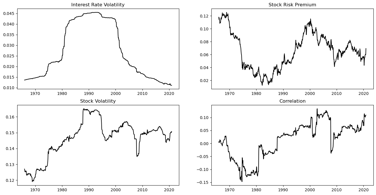
The calibration of the model is similar to the case without ambiguity and incorporates ambiguity by inferring the extreme values for the ambiguous quantities from the extreme values of rolling window estimates. The investor’s time horizon is $T=10$ and the maturity of the bond is $\bar{T}=20$, which is a similar choice compared to other papers on optimal investment with stochastic interest rates [1, 7, 15, 33]. If there is no ambiguity, i.e., when the investor only considers the (constant) scenario $\tilde{\theta}$ (introduced in the previous section), the parameters of the short-term interest rate, the bond, and the stock can be estimated as outlined in Section B of the appendix. Using US data ranging from January, 1946, to December, 2020, the estimation then yields $\kappa=0.336$, $\bar{r}=0.0381$, $\sigma_{r}=0.0262$, $\lambda_{0}^{B}=0.0086$, $\lambda_{S}=0.078$, $\sigma_{S}=0.1457$, and $\rho=0.0196$, which determine the optimal investment strategy neglecting ambiguity. The estimation taking ambiguity into account is based on the same approach but uses rolling window estimates (with a rolling window of 20 years) for the ambiguous quantities (to observe how they vary over time) and then takes the minimum and the maximum of the rolling window estimates as the extreme values for the ambiguous quantities. The variation of the rolling window estimates over time can be seen in Figure 4.1 and leads to the estimates $\underline{\sigma}_{r}=0.0111$, $\overline{\sigma}_{r}=0.0455$, $\underline{\lambda}_{S}=0.0124$, $\overline{\lambda}_{S}=0.1254$, $\underline{\sigma}_{S}=0.1191$, $\overline{\sigma}_{S}=0.1651$, $\underline{\rho}=-0.1474$, and $\overline{\rho}=0.1337$.

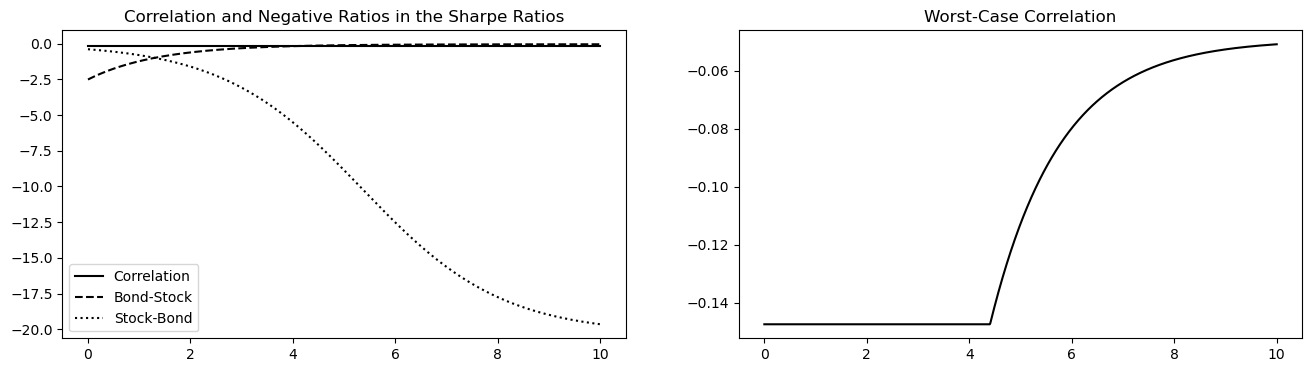
The estimates then enable to compute the optimal investment strategies of an ambiguity averse investor and an investor neglecting ambiguity, respectively. The optimal investment strategy neglecting ambiguity, $\tilde{\pi}$, can be computed using the estimates from the case without ambiguity. In the case with ambiguity, the estimates for the extreme values of the ambiguous quantities determine the worst-case scenario, $\hat{\theta}$, as shown in Theorem 3.1. In particular, the lowest possible correlation, $\underline{\rho}$, and the ratios $-(\underline{\lambda}_{B}(t)/\overline{\sigma}_{r})/(\underline{\lambda}_{S}/\overline{\sigma}_{S})$ and $-(\underline{\lambda}_{S}/\overline{\sigma}_{S})/(\underline{\lambda}_{B}(t)/\overline{\sigma}_{r})$ determine the worst-case scenario for the correlation, which is illustrated by Figure 4.2 and affects the speculative motives of the investor (as described in the cases $(i)$, $(ii)$, and $(iii)$ in the previous section). From the worst-case scenario, one can then compute the optimal investment strategy with ambiguity aversion, $\hat{\pi}$.

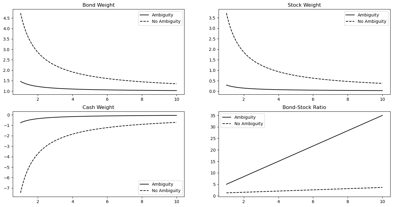
A comparison of the optimal investment strategies at inception shows that ambiguity aversion yields more reasonable positions and preserves the desirable properties of the optimal investment strategy neglecting ambiguity. Figure 4.3 shows the portfolio weights at time $0$ and the related bond-stock ratio as a function of the investor’s level of risk aversion, $\gamma$, corresponding to the optimal investment strategy with ambiguity aversion and the optimal investment strategy neglecting ambiguity. It shows that the ambiguity decreases the bond and the stock weight and increases the cash weight. Thus, ambiguity aversion leads to less leveraged positions compared to the very extreme positions neglecting ambiguity. This is due to the hedge against the ambiguity, which is the distance between the two curves of the risky assets’ portfolio weights at $\gamma=1$. The difference in the portfolio weights is greater for low levels of risk aversion, since then there is more investment in the hedge against ambiguity. Since the hedge part in the bond weight is not affected by the ambiguity, the ambiguity generally increases the bond-stock ratio. The effect is more pronounced for high levels of risk aversion. Therefore, the ambiguity amplifies the effect that the bond-stock ratio is increasing in the relative risk aversion, which is an important result in the asset allocation literature (as pointed out in the introduction) and hence robust with respect to ambiguity.

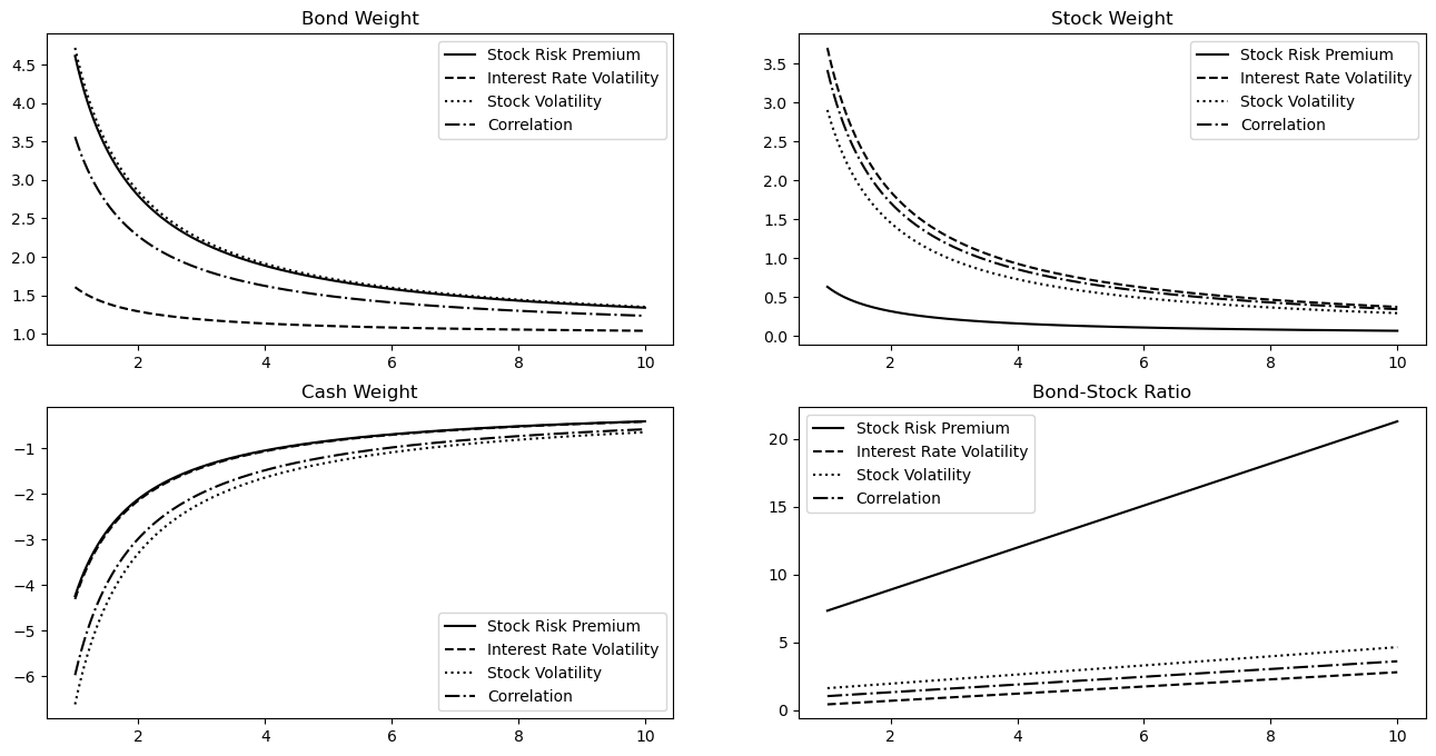
While all sources of ambiguity affect the optimal investment strategy, the magnitude of their effects is different. Figure 4.4 shows the same as Figure 4.3 but for the optimal investment strategy considering only one source of ambiguity for each of the different sources of ambiguity. It shows that the ambiguity about the volatility of the short-term interest rate and the risk premium on the stock have the largest impact on the optimal investment strategy. The ambiguous volatility of the short-term interest rate decreases the bond weight the most compared to the other sources of ambiguity. The ambiguous risk premium on the stock on the other hand has the largest decreasing effect on the stock weight compared to the other sources of ambiguity and consequently has the largest increasing effect on the bond-stock ratio. The reason is that, according to the estimates, the ambiguity about the volatility of the short-term interest rate is relatively large (i.e., the distance between the extreme values relative to the values is large) compared to the ambiguity about the volatility of the stock and that there is more ambiguity (i.e., a larger distance between the extreme values) about the stock’s risk premium compared to its volatility. Despite its magnitude, the ambiguity about the correlation has a relatively modest effect on the optimal investment strategy.

In addition to the static effects, ambiguity aversion also leads to a much more natural dynamic behavior. Figure 4.5 shows the portfolio weights, the speculative part and the hedge part in the bond weight, and the bond-stock ratio as a function of time for $\gamma=2$ corresponding to the optimal investment strategy with ambiguity aversion and the optimal investment strategy neglecting ambiguity. The optimal investment strategy neglecting ambiguity changes only slightly over time (due to the hedge part in the bond weight, which decreases the bond weight and increases the cash weight slightly close to the time horizon) and therefore stays highly leveraged as time passes. The stock weight in the optimal investment strategy with ambiguity aversion increases slightly, as the speculative part shifts from the bond to the stock over time, and then stays constant. The bond weight on the other hand decreases vastly as time passes, since the speculative part decreases (in addition to the hedge part), until the investor stops investing in the bond for speculative reasons, as described in the case $(ii)$ in Section 3, which is illustrated by Figure 4.2, and invests in the bond only in order to hedge interest rate risk. Hence, the cash weight increases over time such that the investor holds almost all wealth in cash at the time horizon, which is intuitive and resembles popular investment advice in contrast to the optimal investment strategy neglecting ambiguity.

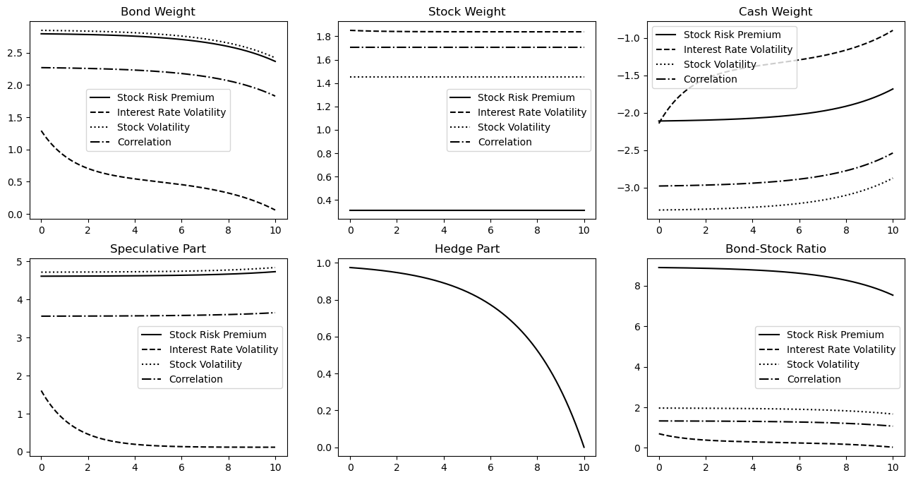
Comparing the different sources of ambiguity shows which source creates the difference in the dynamic behavior of the optimal investment strategy with ambiguity aversion. Figure 4.6 shows the same as Figure 4.5 but for the optimal investment strategy considering only one source of ambiguity for each of the different sources of ambiguity (similar to Figure 4.4 for the static portfolio weights). It shows that the ambiguous volatility of the short-term interest rate is responsible for the change in the dynamic behavior of the optimal investment strategy as it is outlined above. The reason is that the endogenous ambiguity, which is due to the ambiguity about the volatility of the short-term interest rate, causes an additional dynamic effect in the optimal investment strategy, as described at the end of Section 3. The other sources of ambiguity in contrast do not change the dynamic behavior; instead, they make the optimal investment strategy less extreme (similar to the static effects seen in Figure 4.4).

This paper shows the importance and advantages of considering ambiguity–especially several sources of ambiguity–in dynamic asset allocation problems with bonds, stocks, and cash as the main asset classes. On a theoretical level, the results of the paper show that ambiguity aversion in the sense of maxmin expected utility only affects the speculative motives of the investor, which can be interpreted as a hedge against the ambiguity, but it does not affect the demand for hedging interest rate risk. From a practical perspective, ambiguity aversion leads to investment strategies that are more in line with popular investment advice due to the dampening effect of ambiguity in the speculative and highly leveraged part of the investment strategy.

References

- Bajeux-Besnainou et al. [2001] Bajeux-Besnainou, I., J. V. Jordan, and R. Portait (2001). An asset allocation puzzle: Comment. The American Economic Review 91(4), 1170–1179.
- Bajeux-Besnainou et al. [2003] Bajeux-Besnainou, I., J. V. Jordan, and R. Portait (2003). Dynamic asset allocation for stocks, bonds, and cash. The Journal of Business 76(2), 263–287.
- Balter et al. [2021] Balter, A. G., A. Mahayni, and N. Schweizer (2021). Time-consistency of optimal investment under smooth ambiguity. European Journal of Operational Research 293(2), 643–657.
- Biagini and Pinar [2017] Biagini, S. and M. c. Pinar (2017). The robust Merton problem of an ambiguity averse investor. Mathematics and Financial Economics 11(1), 1–24.
- Branger et al. [2023] Branger, N., A. Chen, A. Mahayni, and T. Nguyen (2023). Optimal collective investment: An analysis of individual welfare. Mathematics and Financial Economics 17(1), 101–125.
- Branger et al. [2013] Branger, N., L. S. Larsen, and C. Munk (2013). Robust portfolio choice with ambiguity and learning about return predictability. Journal of Banking and Finance 37(5), 1397–1411.
- Brennan and Xia [2000] Brennan, M. J. and Y. Xia (2000). Stochastic interest rates and the bond-stock mix. Review of Finance 4(2), 197–210.
- Campbell and Viceira [2001] Campbell, J. Y. and L. M. Viceira (2001). Who should buy long-term bonds? The American Economic Review 91(1), 99–127.
- Canner et al. [1997] Canner, N., N. G. Mankiw, and D. N. Weil (1997). An asset allocation puzzle. The American Economic Review 87(1), 181–191.
- Chan et al. [1992] Chan, K. C., G. A. Karolyi, F. A. Longstaff, and A. B. Sanders (1992). An empirical comparison of alternative models of the short-term interest rate. The Journal of Finance 47(3), 1209–1227.
- Dangl and Weissensteiner [2020] Dangl, T. and A. Weissensteiner (2020). Optimal portfolios under time-varying investment opportunities, parameter uncertainty, and ambiguity aversion. Journal of Financial and Quantitative Analysis 55(4), 1163–1198.
- Epstein and Halevy [2019] Epstein, L. G. and Y. Halevy (2019). Ambiguous correlation. The Review of Economic Studies 86(2), 668–693.
- Epstein and Ji [2013] Epstein, L. G. and S. Ji (2013). Ambiguous volatility and asset pricing in continuous time. The Review of Financial Studies 26(7), 1740–1786.
- Epstein and Ji [2014] Epstein, L. G. and S. Ji (2014). Ambiguous volatility, possibility and utility in continuous time. Journal of Mathematical Economics 50, 269–282.
- Flor and Larsen [2014] Flor, C. R. and L. S. Larsen (2014). Robust portfolio choice with stochastic interest rates. Annals of Finance 10(2), 243–265.
- Fouque et al. [2016] Fouque, J.-P., C. S. Pun, and H. Y. Wong (2016). Portfolio optimization with ambiguous correlation and stochastic volatilities. SIAM Journal on Control and Optimization 54(5), 2309–2338.
- Garlappi et al. [2007] Garlappi, L., R. Uppal, and T. Wang (2007). Portfolio selection with parameter and model uncertainty: A multi-prior approach. The Review of Financial Studies 20(1), 41–81.
- Gilboa and Schmeidler [1989] Gilboa, I. and D. Schmeidler (1989). Maxmin expected utility with non-unique prior. Journal of Mathematical Economics 18(2), 141–153.
- Hölzermann [2021] Hölzermann, J. (2021). The Hull–White model under volatility uncertainty. Quantitative Finance 21(11), 1921–1933.
- Hölzermann [2022a] Hölzermann, J. (2022a). Pricing interest rate derivatives under volatility uncertainty. Annals of Operations Research. https://doi.org/10.1007/s10479-022-04921-y.
- Hölzermann [2022b] Hölzermann, J. (2022b). Term structure modeling under volatility uncertainty. Mathematics and Financial Economics 16(2), 317–343.
- Korn [2003] Korn, R. (2003). The martingale optimality principle: The best you can is good enough. WILMOTT July 2003.
- Korn and Kraft [2001] Korn, R. and H. Kraft (2001). A stochastic control approach to portfolio problems with stochastic interest rates. SIAM Journal on Control and Optimization 40(4), 1250–1269.
- Korn and Kraft [2004] Korn, R. and H. Kraft (2004). On the stability of continuous‐time portfolio problems with stochastic opportunity set. Mathematical Finance 14(3), 403–414.
- Kostopoulos et al. [2022] Kostopoulos, D., S. Meyer, and C. Uhr (2022). Ambiguity about volatility and investor behavior. Journal of Financial Economics 145(1), 277–296.
- Lin et al. [2022] Lin, Q., Y. Luo, and X. Sun (2022). Robust investment strategies with two risky assets. Journal of Economic Dynamics and Control 134(1), 104275.
- Lin and Riedel [2021] Lin, Q. and F. Riedel (2021). Optimal consumption and portfolio choice with ambiguous interest rates and volatility. Economic Theory 71(3), 1189–1202.
- Lioui and Poncet [2001] Lioui, A. and P. Poncet (2001). On optimal portfolio choice under stochastic interest rates. Journal of Economic Dynamics and Control 25(11), 1841–1865.
- Maenhout [2004] Maenhout, P. J. (2004). Robust portfolio rules and asset pricing. The Review of Financial Studies 17(4), 951–983.
- Maenhout [2006] Maenhout, P. J. (2006). Robust portfolio rules and detection-error probabilities for a mean-reverting risk premium. Journal of Economic Theory 128(1), 136–163.
- Munk and Sørensen [2004] Munk, C. and C. Sørensen (2004). Optimal consumption and investment strategies with stochastic interest rates. Journal of Banking and Finance 28(8), 1987–2013.
- Rogers [2013] Rogers, L. C. G. (2013). Optimal Investment. Springer.
- Sørensen [1999] Sørensen, C. (1999). Dynamic asset allocation and fixed income management. Journal of Financial and Quantitative Analysis 34(4), 513–531.
- Wachter [2003] Wachter, J. A. (2003). Risk aversion and allocation to long-term bonds. Journal of Economic Theory 112(2), 325–333.