Optimal investment problem for a hybrid pension with intergenerational risk-sharing and longevity trend under model uncertainty
Abstract
This paper studies the optimal investment problem for a hybrid pension plan under model uncertainty, where both the contribution and the benefit are adjusted depending on the performance of the plan. Furthermore, an age and time-dependent force of mortality and a linear maximum age are considered to capture the longevity trend. Suppose that the plan manager is ambiguity averse and is allowed to invest in a risk-free asset and a stock. The plan manager aims to find optimal investment strategies and optimal intergenerational risk-sharing arrangements by minimizing the cost of unstable contribution risk, the cost of unstable benefit risk and discontinuity risk under the worst-case scenario. By applying the stochastic optimal control approach, closed-form solutions are derived under a penalized quadratic cost function. Through numerical analysis and three special cases, we find that the intergeneration risk-sharing is achieved in our collective hybrid pension plan effectively. And it also shows that when people live longer, postponing the retirement seems a feasible way to alleviate the stress of the aging problem.
Key words: robust, hybrid penison, overlapping generations, risk-sharing, longevity trend, model uncertainty.
1 Introduction
Recently, the number of retirees is increasing because of the increasing life expectancy, and there are great pressures on the pension systems due to the change of the economic and demographic. Defined benefit (DB) plans and defined contribution (DC) plans are two traditional types of pension scheme. In a DB plan, plan trustees bear the financial risk while in a DC plan, the participants bear all the longevity and investment risks since they hold their own individual accounts. Furthermore, DC plans are affordable and transparent, as the participants have full control over their contributions. However, they may not obtain adequate benefits upon retirement because their benefits are somewhat depending on the asset returns and interest rates, which could be volatile and unpredictable. On the other hand, DB tends to provide adequate benefits as predetermined. Therefore, they are generally opaque and not necessarily afforable, especially from the plan trustees’ perspective. Thus, neither of these plans is ideal to face the challenges of the demographic transition. The social partners have been planning to revise the regulatory framework for pension funds. An ideal pension scheme should provide adequate benefits and risk-sharing between participants and plan trustees.
Recently, many researchers propose the hybrid pension plan which combines the advantages of DB and DC plans. Hybrid pension plan is in the middle of the two ”extremes” and can be more flexible. Therefore, many countries begin to implement various hybrid pension plans. For example, the collective DC plans (Kortleve (2013); Bovenberg et al. (2014)), target benefit plans (Munnell and Sass (2013); Wang et al. (2018)), risk-sharing DB plans (Pugh and Yermo (2008)), the floor-offset plans ( Chen and Hardy (2009)) and Notional Defined Contribution (NDC) plans (Alonso-Garcia and Devolder (2016), Alonso-Garcia et al. (2018)). Turner and Center (2014) provide an overview of the development of hybrid pension plans around the world and classify the plans into four different types: the hybrid DB plans in the Netherlands, the nonfinancial DC plan in Sweden, cash balance plans in the United States, Canada and Japan, and the Riester plans in Germany.
The hybrid pension plan aims to provide a better retirement security on a sustainable, stable and affordable basis with risk sharing among different age cohorts. Actually, it is well documented that intergenerational risk-sharing may be welfare enhancing. Gollier (2008) proves that intergenerational risk transfer is welfare-improving for all current and future generations in a collective pension scheme compared with participants in individual schemes. This is because a better intergenerational risk-sharing scheme makes it socially efficient to raise the collective risk exposure in order to take advantage of the large equity premium. Cui et al. (2011) examines a funded system with a realistic description of risks in financial markets. Comparing risk sharing in various types of funded pension systems such as individual DC plans, collective DC plans and traditional DB plans, they find that risk-shifting over time (due to adjustment mechanisms) leads to higher utilities in pension schemes. Jean-Franois (2020) studies intergenerational risk and cost sharing for a variety of collective funded pension plans with time-varying contributions and benefit levels considering the Volatility Index (VIX). He also concludes that pension schemes with a well-structured volatility-risk-adjusted component can be welfare enhancing for the entry and future cohorts. Similar researches can be found in Teulings and De Vries (2006), Beetsma et al. (2012), Beetsma (2016), Boes and Siegmann (2018). Besides, there are other studies in the literature having tried to find optimal contributions and/or benefit adjustment policies within hybrid pension funds. See Khorasanee (2012), Wang and Lu (2019), He et al. (2020) and the references therein.
Furthermore, the issue of longevity is an important factor when designing intergenerational risk-sharing scheme. The increasement of people’s average life expectancy poses a threat to the traditional pension plans. Strulik and Vollmer (2013) show that improvements in life expectancy have been driven to a large part by expansions of the maximum age from the second half of the 20th century onwards. Therefore, Knell (2018) thinks that a straightforward way to capture increasing life expectancy is to assume that the maximum age increases in a linear fashion according to time. Devolder and Melis (2015) introduce the factor that is a random effect on the expected survival probability to reflect systematic longevity risk in a two-period model. Besides, it captures the longevity trend through the force of mortality that is not only age-dependent but also include a cohort-specific time. To be more specific, in the long run, people’s force of mortality is relatively low due to the progress of medical treatment and development of economy. On the other hand, it is obvious that the force of mortality raises when people’s age increases. Furthermore, Knell (2018), Alonso-Garcia and Devolder (2019), Andrés et al. (2014) and Holzmann et al. (2017) all take the socio-economic status and income into consideration in model of mortality. Inspired by Knell (2018), we assume that the maximum age is an incresing function of the time in this paper. Moreover, we apply an a age and time-dependent force of mortality which we call modified Makeham’s Law to capture the longevity.
Traditionally, the manager of the hybrid pension plan is assumed to know exactly the true probability measures of financial market. However, decision-makers are uncertain about the true model in practice. Because, for example, the parameters (especially the drift parameters) are hard to estimate with precision (Merton (1980)). Therefore, it is fair to say that any particular probability measure used to describe the model would be subject to a considerable degree of model misspecification. This type of uncertainty caused by the lack of information about the probability measure is also referred to as ambiguity, which is apparently different from risk where the model is characterized by a single probability measure. To deal with the decison makers’ ambiguity aversion, Anderson at el. (2003) proposes a robust control approach in a continuous-time framework. They assume that the decision-maker does not trust the specific probability measure. and treats it as a reference measure, and takes into account a set of alternative measures that is statistically difficult to distinguish from the reference measure. The gap between the reference measure and an alternative measure is constrained by the relative entropy, which acts as a penalty term in the optimization procedure. This penalty captures the decision-maker’s ambiguity aversion about the reference measure. Rencently, Wang and Li (2018) investigate a robust optimal investment problem for an ambiguity-averse member of defined contribution (DC) pension plans with stochastic interest rate and stochastic volatility. In addition, Wang Peiqi et al. (2021) consider the optimal investment and benefit payment problem for a target benefit plan (TBP) with default risk and model uncertainty.
However, to the best of our knowledge, there is few literature on investment problem of hybrid pension plan under ambiguity. But the plan manager is always uncertain about the reference model. Therefore we assume that a representative hybrid plan member is ambiguity averse in this paper. Suppose that all the participants are in an aggregate pension fund with both active members and retirees in an overlapping generations’ economy. Contributions are paid by active members and at the same time the retired members receive benefits from the pension fund. It is more reasonable that all generations should share the risk and this is achieved by adjusting contributions and benefits as a function of the fund surplus which is the difference between the asset and target liability. This adjustment scheme is motivatied by real-world example (see e.g.Ponds and Van (2007)). In this collective hybrid pension scheme, we focus on the strategic portfolio allocation decisions together with pension policies, that are intergenerational risk sharing rules, to dynamically adjust financial position of the pension funds. Inspired by Wang and Lu (2019), the ultimate goals of this study is to provide retirees adequate and stable retirement benefits and to ensure fair and effective contributions from active members. Meanwhile, plan manager is ambiguity averse and aims to keep the system financially sustainable ensuring the generational equity under the uncertainty. Mathematically, these goals are achieved through minimizing the expected utility of intergenerational risk, adjustment of the contribution and the benefit, which is called the discontinuity risk, the unstable contribution risk and the unstable benefit risk, respectively, by choosing appropriate cost function under the worst-case scenario. According to Haberman (1997), Josa-Fombellida et al. (2001) and Ngwira and Gerrard (2007), we consider the quadratic cost function.
The contributions of this paper is as follows. First of all, we take model uncertainty into account, which reflect the fact that in many situation decision-makers are uncertain about the true model, and try to find the robust strategy for the pension plan under the worst-case scenario. Then, the model we considered, comparing to Cui et al. (2011) and Khorasanee (2012), is in an overlapping generations’ economy (OLG). This OLG model allows people to enter and leave at every continous time and all the generations will share the risk together. Besides, we consider the age and time-dependent force of mortality that is the modified Makeham’s Law, which reflects the longevity trend of population. At last, followed by He et al. (2020), we consider the negative entrant growth rate of the labor supply, which could reflect the fact of low fertility.
The rest of the paper is structured as follows. In Section 2, we introduce the model of financial market and the hybrid pension plan. In Section 3, we propose the optimal investment problem for the hybrid pension and robust strategy under model uncertainty. In Section 4, we give three special cases. In Section 5, we present some numerical results and sensitivity analysis. Finally, Section 6 concludes the paper and provide some further research ideas.
2 Model formulation
Let be a complete probability space, where is a complete and right continuous filtration generated by a two-dimensional standard Brownian Motion, that is, is the filtration containing the information about the financial market and the information about the salary of the members at their time of retirement at time , which is available to the sponsor of the pension plan, and is a probability measure on .
2.1 The financial market
The financial market consists of a risk-free asset (bond) and a risky asset (stocks). The price of the risk-free asset and risky asset at time is described by
| (2.1) | |||
| (2.2) |
where denotes the risk-free interest rate. is the appreciation rate of the stock and is the volatility rate, both and being positive constants, and is a standerd Brownian motion. To exclude arbitrage opportunities, we assume that .
2.2 Population dynamics
For population, We will develop a continuous deterministic framework considering that age and time are continous variables. Plan members are assumed to enter the labor market at age and to keep active up to a retirement age . As above mentioned, it is reasonable that the force of mortality decrease with time and increase with age because of the decreasing fertility and increasing life expectancy. Here, we consider an age and time-dependent mortality followed by modified Makeham’s Law, which may capture longevity trend dynamically as following assumption.
Assumption 2.1
The age and time-dependent force of mortality is denoted by
where is a positive parameter called longevity parameter which shows longevity trend that is every year, the average life expectancy increases by one year. More precisely, for a -year-old cohort at time 0, the force of mortality is . years later, the force of mortality at time is . And theoretically, if there is no longevity parameter, the force of mortality at time could be like . Therefore the model we considered shows that people have relatively low force of mortality and is equivalent to be one-year “younger”. On the whole, the average life expectancy would increases by one year.
Remark 2.1
In this age and time-dependent force of mortality, we note that the higher , the trend of longevity comes more slowly which means it takes long time for the whole people be long-lived. Instead, the lower , the aging problem would be more urgent. For example, according to European Commission (2015), for the European Union(EU)-countries, life expectancy at birth is projected to increase over the next 50 years by about 7.5 years, which means almost .
Assumption 2.2
The maximum age is denoted by
where is the initial maximum survival age.
This assumption shows that the maximum age increases in a linear fashion and is in line with the empirical literature. Knell (2018) and Oeppen and Vaupel (2002) e.g., analyze ‘record female life expectancy’ (i.e., the highest value for female life expectancy reported in any country for which data are available) from 1840 to 2000 and they show that it follows an almost perfect linear development. Actually, Strulik and Vollmer (2013) have shown that from the second half of the 20th century onwards improvements in life expectancy have been driven to a large part by expansions of the maximum age.
Denote the survival function that the cohort who enter the system at time survives to age . It holds that and that survivorship declines with age, i.e., for . The mortality hazard rate of cohort at age is given by
therefore, and are not only age-specific but also include a cohort-specific time index. It holds that:
Thus the age and time-dependent survival function can be expressed as
| (2.3) |
We denote by the entry rate which describes the density of sizes of new cohort entering in working life at age at time . follows Malthusian demographic model , where is the density of the new -year-old entrants at time , is the growth rate of the new entrants. Inspired by He et al. (2020) and He et al. (2021), represents the demographic model with serious aging problem, which is caused by low fertility and low mortality. Then the number of those attaining age at time is
where is the time at which this cohort joined the pension system. Note that with , the value of could be negative, meaning that a member whose age is at time joined the pension system years ago. The total number of active member who make contributions at time is given by
| (2.4) |
and the total number of retired members who recieve the benefits at time is
| (2.5) |
Here, we assume that during the working period, each cohort receives his labor income, which is normalized to 1. Therefore the total contribution income is
| (2.6) |
and the total benefit payment is
where and is the amount of the contribution and benefit at time t, respectively. The specific forms about and will be given by the next section.
Remark 2.2
The surplus (deficit) between the total contribution income and the total benefit payment will increase (decrease) the accumulation of the pension fund. Meanwhile, the accumulation is dynamically allocated to a risk-free asset and a risky asset.
2.3 Hybrid pension scheme
The pension fund trustee is responsible for the asset-liability management. The amount of money invested in the risky asset at time is denoted by and then the amount invested in risk-free asset is . The dynamics of the asset process can be described by
| (2.7) |
where is the initial asset at time 0. Using (2.1) and (2.2), we can easily rewrite (2.7) as
| (2.8) |
Consider the target contribution and target benefit at time and a finite time interval with being the so-called terminal time. For each age cohort, denoted by , the target liability equals the difference between the present value of risk-free benefits and the present value of the yet-to-be-paid risk-free contributions. This is in line with the one in the literature of Cui et al. (2011).
| (2.9) |
where is the target instantaneous growth rate of the target contribution and the target benefit.
At the aggregate level, the target liabilities of the fund can be calculated simply as the sum of the liabilities for each age cohort.
| (2.10) |
Given the sationary age composition of the fund and the fixed target benefit level, the target liability is time invariant. Actually, if the fund invests fully in the risk-free asset, then the actual liability follows exactly as the target liability . If the fund accepts mismatch risk, for example by investing in stocks, there may be funding surpluses or deficits with respect to the target liability.
The fund surplus is defined as the diference between assets and the target liability level
Notice that the collective pension schemes may leave surpluses or deficits which lead to intergenerational transfers and hence to intergenerational risk sharing.
Besides the adjustment of the plan members’ traget liabilities as described in (2.10) by linking to the fund assets as decribed in (2.8), for the collective hybrid pension model, we also dynamically and simultaneously adjust both the current individual contribution paid by the active members and individual benefit payments payable to the retirees, implicitly influenced by the surplus level of the pension fund in order to make intergenerational risk sharing.
To achieve our goal mentioned above, we specify a simple cohort contribution and benefit policy, where the contribution per cohort is a function of the target contribution rate level and the funding residual per active cohort , and the benefit per cohort is a function of the target benefit rate level and the funding residual per retire cohort .
| (2.11) | |||
| (2.12) |
where , which represent the adjustments to the pension contributions and benefit payments, respectively. The slope coefficient and change over time according to the adjustment of the hybrid pension system thus reflect the speed of absorbing the funding imbanlances, being the so-called spread parameters for contribution income and benefit payment, respectively. or implies that a funding imbalance is immediately and fully abdorbed. More specifically, a fraction of the funding residual is shared among employees and a fraction of the funding residual is shared among retirees. A lower vaule of and imply that part of the funding surplus is shifted to the future, and shared across generations i.e. the lower vaule of and , the higher the degree of intergenerational risk sharing.
The two adjusted processes and describe the pension system over the time which consist of decision on contribution and benefit payment for each cohort at time . When the underlying fund value at time t has surplus (), indicating an out performance in assets investment, we expect both positive policy adjustment of and so that at time t the benefit payments would be increased while the contributions required being decreased. When the underlying fund incurs a deficit due to investment losses (), we in turn expect both negative policy adjustment of and . Here, increasing the contributions and decreasing the benefits can re-balanced the budget. All in all, high and low asset returns of the fund are spread over active members and retirees, which implies an intergenerational risk transfer or sharing. Such hybrid pension model has a similar mathematical structure as the hybrid model studied in Cui et al. (2011), Khorasanee (2012) and Wang and Lu (2019).
In the following section we present, for the pension model described above, we set a continuous-time robust stochastic optimal control problem for the hybrid pension plan.
3 Optimal investment problem for the hybrid pension under model uncertainty
3.1 Optimization problem
In the traditional framework of pension plan or investment problem, the member is assumed to be ambiguity-neutral, which implies that the manager has complete confidence in the above model provided by probability measure . However, the fact is that in many cases the member cannot know exactly the true model, and thus any particular probability measure used to describe the model would lead to potential model misspecification. The parameters of financial markets are difficult to estimate with precision in practice and numerous experimental studies demonstrate that the investors are averse not only to risk (the known probability distribution) but also to ambiguity (the unknown probability distribution) (refer to Peter et al. (2010)). Therefore, we assume that the manager is ambiguity-averse and aims to protect himself against the worst-case scenario. The manager recognizes that the models under the reference probability only approximate the true models and takes into account some alternative models, which can be defined via a family of probability measures equivalent to as follows
Based on this assumption, we can use Girsanov’s theorem to change the probability measures, so that the models defined by the alternative measures only differ in terms of drift function. By Girsanov’s theorem, for each , there is a progressively measurable process , which can be referred as the probability distortion process, such that
where
| (3.1) |
Moreover, if satisfies Novikov’s condition
then the Radon-Nikodym derivative process is a -martingale.
According to Girsanov’s theorem, under the alternative measure , the stochastic process is one-dimensional standard Brownian motion, and we have
Hence, for the given measure , choosing an alternative measure is equivalent to determining the process . Furthermore, the price of the stock and dynamic asset process under alternative measure become
| (3.2) | ||||
| (3.3) |
Definition 3.1
(Admissible Strategy). For any fixed , a strategy
is said to be admissible if
-
(i)
is -adapted;
-
(ii)
for all , and ;
-
(iii)
is the unique solution to SDE (2.8).
Recall that the hybrid pension plan considered consists of both active members who make contributions to the fund and retired members who receive pension benefits. Since the contribution and benefit are time variant, the plan trustees must choose an asset allocation, contribution and benefit strategies which strike a reasonable compromise between the interests of these two groups. Ideally, the fund should make contributions and benefits in a stable and sustainable manner to each cohort as close to the target as possible. As the pension plan we considered is a collective one with different generations involved, taking the all generations into consideration, the goal of the pension trustees is that the pension plan can be run stably and sustainably and the investment risks are shared intergenerationally.
Mathematically, the objective of this continuous-time hybrid pension system is to seek a robust optimal strategy to minimize the expected discounted cost of unstable contribution risk, unstable benefit risk and discontinuity risk over the time interval . The model setting is in line with He et al. (2020) and Wang et al. (2018). In particular, the contribution and benefit should be stable and comparable with respect to target contibutionn and target benefit, and the final accumulation should be neither too large nor too small, comparing with the initial accumulation. As such, we propose a cost function that consists of three parts. The first part is the deviation between the actual contribution and the target contribution. The target contribution is a reference level, At any time , when is ralatively larger (smaller) than , the current working cohorts (cohorts at previous times) naturally feel unstatisfied because of bearing higher contribution burden, comparing to the cohorts at previous times (current working cohorts). In this cricumastance, there is welfare cost due to the unstable contribution risk. The second part is the deviation between the actual benefit and the target benefit. As same as the first part, should aproach the as much as possible in order to make sure that is fair to all the cohorts. If not, in this cricumastance, there is also welfare cost due to the unstable benefit risk. The third part is the initial accumulation to depict the cost of the two risks. When the final accumulation is smaller (larger) than the initial accumulation, there exist intergenerational transfer from the current working cohorts (cohorts at other times) to the cohorts at other times (current working cohorts), In this circumstance, there is welfare cost due to the discontinuous accumulation risk. Hence, the objective is to minimize the deviations within the finite time horizon . In the literature Josa-Fombellida et al. (2001), Ngwira and Gerrard (2007) and Wang et al. (2018), both the finite and infinite time horizon are studied, and the finite time horizon vary from years to decades. In this paper, we assumed a reasonable finite time horizon because that the pension manager pays more attention to the interests of the working cohorts in their term of mangement, which means that they do not take the interests of the unborn into consideration. Further reasons about finite time horizon can be found in He et al. (2020). Employing the quadratic deviations as the cost function, We formulate the robust optimal investment problem as follows:
| (3.4) |
where is a set of all the admissible strageies of . , and are nonnegative constants, interpreted as the weight parameter which measures the importance of the cost of unstable contribution risk, the cost of the unstable benefit risk and the cost of the discontinuous risk in the overall cost function, respectively. The expectation is computed under the alternative measure defined by . The last part in (3.4) is the penalty term depending on the relative entropy which measures the discrepancy between the alternative measure and the reference measure, and the increase in the relative entropy from to equals . This integral term is scaled by which is nonnegative and stand for the preference parameters for ambiguity aversion, measuring the degree of confidence to the reference probability . The larger is, the more ambiguity-averse the insurer is, the smaller the penalty for deviating from the reference measure is, and the less faith in the reference measure the manager has. Finally, when , the manager is completely convinced that the true measure is the reference measure . In this case problem (3.4) degenerates to the classical the quadratic deviations minization in the absence of ambiguity. When , the penalty term vanishes, which implies that the member is extremely ambiguous (see Uppal and Wang (2003); Yi et al. (2014);Wang and Li (2018)). And for analytical tractability, we assume that , where is positive constants and stand for the ambiguity aversion parameter, meaning manager’s the different levels of ambiguity aversion about the stock’s price.
Thus, the continuous-time robust stochastic optimal control problem for the hybrid pension plan is established. By choosing strategies, the manager seeks to minimize the penalized objective function in the worst-case scenario. In the section below we aim at finding the optimal policy which solves the optimal control problem.
3.2 Robust strategy to the optimization problem
In this section, we use standard methods to solve the optimal control problem (3.4) and derive closed-form expressions of the optimal policy, denoted by , within all the admissible policies.
First, we define a variational operator
| (3.5) |
where , , are partial derivatives of .
According to the principle of stochastic dynamic programming, the Hamilton-Jacobi-Bellman (HJB) equation can be derived as(see Uppal and Wang (2003); Yi et al. (2014)):
| (3.6) |
Based on the above setting, we derive a solution to the HJB equation (3.6) with . We state our findings on the optimal asset allocation, contribution and benefit adjustment policies for robust optimal control problem (3.4) in the following theorem. For notation simplicity, we let , which is the Sharpe ratio of the risky asset.
Theorem 3.1
For the optimal control problem (3.4), the optimal asset allocation policy, contribution and benefit adjustment policy are given, respectively, by
| (3.7) | ||||
| (3.8) | ||||
| (3.9) | ||||
| (3.10) |
where and is show as (2.4) and (2.5) respectively. and the corresponding value function is given by
| (3.11) |
where the expressions of and are given below. We denote that
| (3.12) |
then and can be show as
| (3.13) |
where
| (3.14) |
Proof. According to the first-order optimality conditions, differentiating expression in bracket of (3.6) with respect to , the function is given by
| (3.15) |
Substituting (3.15) into (3.6), we have
| (3.16) |
Differentiating expression in bracket of (3.6) with respect to , and , setting to zero and solving them give immediately
| (3.17) |
Substituting (3.17) into (3.16), denote
we have
| (3.18) |
To solve (3.18), we try to speculate on the solution in the following form
| (3.19) |
whose partial derivatives are
| (3.20) |
Substituting (3.20) into (3.18), the optimal policies (control variables) can be expressed in terms of the functions , .We have
| (3.21) |
The coefficients of , are all zeros, which leads to the following system of differential equations
| (3.22) |
Differential equations (3.22)with boundary conditions in (3.19) can be easily solved. Denote , we have
| (3.23) |
where
| (3.24) |
Above, we have derived closed-form expressions for the optimal investment strategy and optimal risk-sharing arrangemnts taking into account the three competing objectives of contibution rate stabilty and benefit stability and continous intergenerational risk-sharing.
Remark 3.1
According to the closed-form result, it is not so obvious about the impact of the longevity parameter . Actually, the ,, is closely ralated to the , since the expression of and contain survival function where as the important longevity parameter being shown in the force of mortality.
Then, we will interpret the optimal controls presented in (3.8), (3.9) and (3.10), providing economic intuition for some of their more surprising behavior.
First, in (3.22) can be rewrite in actuarial notation as
where is the present value of an annuity certain payable continuously for the remainder of the horizon, valued at a force of interest . Besides, in (3.12) represent the difference between the target total contribution and target total benefit. Therefore the first term in is the present value at time of difference between the target total contribution and target total benefit during the remaining horizon, and the second is the accumulated asset at time for the initial fund. Now, we can have next remark.
Remark 3.2
The expression for in (3.8) can be rewritten as a constant proportion () of the excess or shortfall of its total assets and the present value of the plan’s aspirations.
Here total assets include both its financial assets and the present value of defference between the target total contribution and target total benefit which will collect over the remainder of the horizon, whereas the plan’s “aspirations” reflects the target accumulated assets, with all items being valued at the risk-free rate, which is in line with Wang et al. (2018). Consequently, investment in the risky asset is required only when the plan’s total assets are not sufficient to cover the plan’s aspirations by investing exclusively in the risk-free asset.
Next, moving our focus to the optimal risk-sharing adjustment policy. Like , can also be rewrite in actuarial notation as
| (3.25) | ||||
| (3.26) |
where and is the present value of an annuity certain payable continuously for the remainder of the horizon, valued at a force of interest . Therefore
where the denominator represent the present value of a continuous investment of at time for years, valued at the adjusted rate , while leaving a lump sum at the end of years equal to , valued at the adjusted rate . And can be showed as same way.
Remark 3.3
The expressions for and have similar pattern, and multiplying both side by () in 3.9(3.10), we have
and we find that the optimal total contribution adjustments and optimal total benefit adjustments at time are dynamic adjustments that spreads the current excess (shortfall) of the plan’s total assets relative to the plan’s aspirations over the remaining number of years in the horizon with a proportionate share left over as part of the legacy fund at the end of the horizon.
4 Special Cases
4.1 Optimal investment problem for a hybrid pension without model uncertainty
Under the assumptions of no uncertainty, as we mentioned in section 3.1, when in (3.4) , the manager is completely convinced that the true measure is the reference measure . In this case, problem (3.4) degenerates to the classical quadratic deviations minization in the absence of ambiguity. since , where is positive constants and stand for the ambiguity aversion parameter, meaning manager’s the different levels of ambiguity aversion about the stock’s price, therefore, we can set in problem (3.4). The following is the classical quadratic deviations minization problem in absence of model uncertainty.
| (4.1) |
The result of problem (4.1) is given by following Theorem (4.1), which is derived by set in Theorem 3.1.
Theorem 4.1
the optimal asset allocation policy, contribution and benefit adjustment policy are given, respectively, by
| (4.2) | ||||
| (4.3) | ||||
| (4.4) |
where and is show as (2.4) and (2.5) respectively. and the corresponding value function is given by
| (4.5) |
where the expressions of and are given below. We denote that
| (4.6) |
then and can be show as
| (4.7) |
where
| (4.8) |
Remark 4.1
and are unaffected by uncertainty, and is associated with uncertainty. It can be seen that the proportion of investment in risky assets decreases with the increase of time and is lower than when there are exist model uncertainty. The contribution is lower than that with model uncertainty, and the retirement benefits are higher than that with model uncertainty. This is mainly because pension managers have confidence in the model and do not have the risk of model uncertainty. For detailed analysis, see numerical analysis in section 5.
4.2 Optimal investment problem for a hybrid pension without consideration of longevity trend
Under the assumptions of on longevity trend, we can set in Assumption 2.1 and in Assumption 2.2. Therefore the maximum survival age is which is constant and the survival function is denoted by
| (4.9) |
which is as same as the Wang and Lu (2019). Besides, the optimal investment problem is as same as the (3.4) which is given by
| (4.10) |
Theorem 4.2
The optimal asset allocation policy, contribution and benefit adjustment policy are given, respectively, by
| (4.11) | ||||
| (4.12) | ||||
| (4.13) | ||||
| (4.14) |
where and is show as
| (4.15) |
and the total number of retired members who recieve the benefits at time is
| (4.16) |
where the is given by (4.9).
The corresponding value function is given by
| (4.17) |
where the expressions of and are given below. We denote that
| (4.18) |
then and can be show as
| (4.19) |
where
| (4.20) |
Remark 4.2
and were affected by the longevity trend, while was not. It can be seen that the proportion of investment in risky assets is lower than that with longevity trend, the optimal contribution is lower than that with longevity trend, and the optimal retirement benefits are higher than that with longevity trend. The main reason is that without the influence of longevity trend, the pension system has no aging problem, while the actual pension system has the influence of longevity trend. Therefore, pension systems with longevity trends must be considered. For detailed analysis, see numerical analysis in section 5.
4.3 Optimal investment problem for a hybrid pension without model uncertainty and consideration of longevity
Under the assumptions of without uncertainty and longevity trend, we set , , . The optimal investment problem is as same as (4.1) and is given by
| (4.21) |
Theorem 4.3
the optimal asset allocation policy, contribution and benefit adjustment policy are given, respectively, by
| (4.22) | ||||
| (4.23) | ||||
| (4.24) |
where and is show as (4.15) and (4.16) respectively. and the corresponding value function is given by
| (4.25) |
where the expressions of and are given below. We denote that
| (4.26) |
then and can be show as
| (4.27) |
where
| (4.28) |
5 Numerical illustrations
In section 3, we have establish the explicit expression of the robust optimal investiment allocation and adjustment strategies of both the contribution and the benefit for per cohort in the hybrid pension model. In this section, we present numerical examples to illustrate our results regarding optimal policies.
The parameter settings in numercial simulation are mainly in line with the ones in literature Wang and Lu (2019). In the demography aspect, we assume a negative growth rate of new labor entrants to study the impacts of aging problem (), which depicts the scenario of negative growth of labor supply. The assumption is far removed from current reality but might emerge soon. For the age and time-dependent survival function, set , , . Besides, we set , which means that every 4 years, the average life expectancy increases by one year.
| -0.005 | 1.124 | 0.000022 | 4 | 25 | 65 | 10 | 3000 | 20 | 100 | |
| 0.1 | 0.7 | 0.02 | 2 | 2 | 2 | 0.01 | 0.05 | 0.15 | 2 | 0.25 |
In the pension rules aspect, the age of the new entrants into the pension system is , and the age of retirement is . The number of new entrants at time 0 is . The initial fund accumulation is . The time horizon is . Futhermore, the target contribution is , and target benefit is . And the target growth at detemnistic rate . We assume that the weight parameter , and we will change the vaule and analyse the impact.
In the finacial market aspect, the risk-free interest rate is . The expected return and the volatility of the risky asset is and , respectively. As such, the sharpe ratio is . At last, the ambiguity aversion parameter .
In the following part, we use Monte Carlo method to do the numerical analysis. We first partition the time interval into 1000 subintervals, For each of these subintervals, we generate a random variable with normal distribution, which applied to the common random source of risky asset. Based on the salary level and risky asset price, as well as the optimal control policies obtained in section 3, we could get the new fund accumulation at the end of the subinterval. Then, we recalculate the optimal contribution, the optimal benefit and the optimal asset allocation amount based on the new accumulation, using (2.11), (2.12), (3.8), (3.9), (3.10), following the above instructions, the procedure is repeated in the next subinterval using the newly determined value of , yielding 1000 consecutive values of during the time interval . By repeating this process 1000 times, we obtain the empirical distribution of at the end of each subinterval, and the average of the optimal contribution rate , the average of the optimal benefit and the average of the optimal risky investment proportion are used by the follow-up analysis.
According to the parameter settings in the Table 1. Figure 1 gives the information about the spread parameter for rcontribution income and benefit payments , in the hybrid pension system. Both the and have similar trend. As we mentioned in section 2, the lower vaule of and , the higher degree of intergenerational risk sharing. As such, the pension system gradually decreases the part of funding surplus which shifted to the future, i.e, decreases the degree of intergenerational risk sharing.


In the first part of sensitivity analysis, we study the impacts of demography trends and time interval on the optimal control policies with respect to time .
First, we investigate the impacts of new entrants growth rate on the optimal polices for the hybrid pension model. In Figure 2, when the new entrants growth rate is decreases, the dependency ratio increases and it leads to higher deficit of the pension budget. As such, the contribution substantially increases and benefit decrease at the same time. In Figure 3, when the new entrants growth rate decreases, the proportion allocated to the risky asset increases. The pension manager needs to take more investment risk to re-balance the pension budget. Besides, we notice that when which means that the number of population entering the pension plan system is every year and the population stays relatively stable during this 20 years. In that case, In the first two years, the contribution and optimal investment proportion are negative since there are no much pressure on finacial at the beginning.


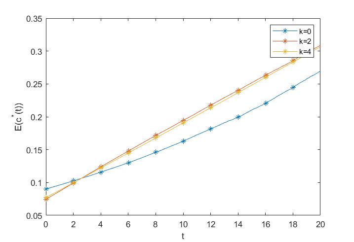
Then, we investigate the impact of time interval on optimal policies. In Figure 4, long time interval leads to higher contribution and lower benefit since there are more uncertainty in the remote future and we have to put sufficent money into pension system to meet the budget. In Figure 5 (a), when time interval we considered is relatively long, there are more proportion put into risky asset since pension system needs more money to keep sustainable.

In the second part of sensitivity analysis, we study the cross impacts of two dimensional parameters on the optimal policies at time 10.
First, we investigate the impacts of retirement age and longevity parameter on optimal policies. In Figure 6 and Figure 7 (a). Lower means the aging problem is relatively urgent, which leads to higher contribution, higher risky asset proportion and lower benefit. That is because there will be more retired people in our system, higher contribution and risky asset proportion can increase the asset so that keep our pension system stable and sustainable. At the same time, if we can postponing retirement age, the risky asset proportion and contribution will slightly decrease and the benefit will increase, since there are more working cohort in pension system and sufficient accumulations as the benefit payment. This can alleviate the contribution burden and reduces both of the risk-taking and discontinutity risk in some aspects. Therefore, according to the change of longevity parameter , we can choose the appropriate retirement age to make sure the pension system run smoothly.


Second, we investigate the impacts of retirement age and new entrants growth rate on optimal policies. In Figure 7(b) and Figure 8, when the new entrants growth rate is low and people retire early, the contribution rate and the risky investment proportion are both high. Meanwhile, we find that postponing the retirement age from 60 to 70 could offset the negative impact of decreasing new entrants growth rate from 0.01 to -0.01. Therefore, postponing the retirement is an important measure to alleviate the adverse influence of the aging problem. This conlusion is in line with the He et al. (2020).


At last, we investigate the impacts of the weight parameter of unstable contribution and benefit risk on optimal policies. In Figure 9, when is high and is low, which means we are more care about the unstable contribution risk instead of unstable benefit risk, both the contribution and benefit are high. This shows that as long as keeping the contribution stable and adequate, the benefit is natually can be statisfied.


In the third part of sensitivity analysis, we study the special cases that we discussed in Section 4.
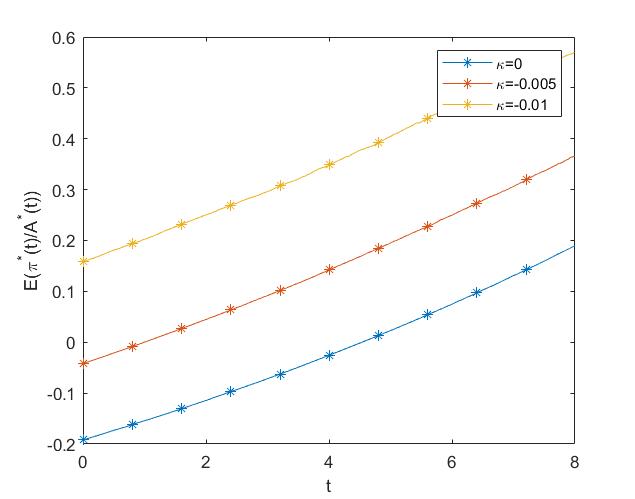
First, under the assumptions of no uncertainty, Figure 10 and 11 is the numercial analysis compared with the and . When there is no model uncertainty, the contrubtion is relatively low and the benefit is raltively high. Besides, the investment proportion has a total different pattern. That is because the pension manager has faith to the true model and no risk of model uncertainty.


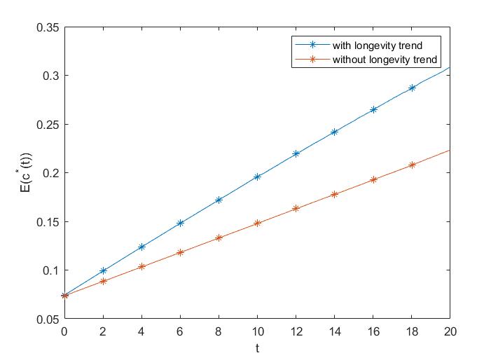
Then, under the assumptions of on longevity trend, Figure 12 and 13 is the numercial analysis compared with the model with longevity trend. When there is no longevity trend, the contrubtion and investment proportion is relatively low and the benefit is raltively high. Without longevity trend, there are not too much pressures on the pension plan, therefore, it allows that a few proportion of assets invested to the finicial market.


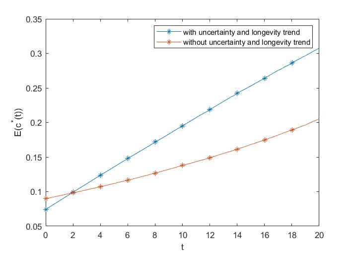
At last, under the assumptions of without uncertainty and longevity trend, the contrubtion is relatively low and the benefit is raltively high. Besides, the investment proportion has a total different pattern. Without uncertainty and longevity trend, pension manager has faith to the true model and no pressure of aging problem. Thus, it is reasonable to decrease the proportion of investment to risk asset and the contributions, and retirees can get more pension after they retired which is in line with the He et al. (2020) and Wang et al. (2018).


6 Conclusion
This paper investigates the optimal contribution, the optimal benefit payment and the optimal asset allocation policies to minimize the cost of unstable contribution risk, the cost of unstable benefit risk and discontinuity risk in a hybrid pension plan under model uncertainty. Considering that all the participants are in an aggregate pension fund with both active members and retirees in an overlapping generations economy, we propose a dynamic and controllable model for this hybrid pension fund. Besides, a linear fashion of maximum survival age and an age and time-dependent force of mortality is considered to capture the longevity trend which is decrease with time and increase with age. The fund asset is invested in a risk-free asset and risky asset, and we employ the penalized quadratic deviations as the cost function. By adjusting both the contribution rate and benift according to the surplus or deplict (the difference between the fund asset and the target liabilities), the fund residual can be shared across generations, including employees and retirees. Solving the minimization problem by HJB under the worst scenario, we obtain the robust optimal strategies in our hybrid pension plan. In the part of numercial illustrations, we investigate the impact of different parameters. In most cases, there are opposite trends between the contribution rate and the benefit, since the pension fund should always be stable and balanced. Include, the time interval have a positive impact on contribution and risky aseet proprotion, which means we must have sufficient money to face the long-term hybrid pension system. Besides, Postponing the retirement age could offset the negative impact of decreasing new entrants growth rate, which lead to lower contribution and higher benefit. Therefore, postponing the retirement is an feasible measure to alleviate the aderverse influence of the aging problem. In the section of three special cases, we notice that taking the uncertainty and longevity into consideration increase the proportion of investment to the risk asset and contributions, and decrease the benefits.
However, there are still many aspects that can be researched in our future study. Firstly, we assume that the force of mortality is age and time-dependent. This hypothesis is reasonable due to the decreasing fertility and increasing life expectancy. Furthermore, it is worth mentioning that some research has emphasized the relationship between socio-economic status, income and mortality; see, Andrés et al. (2014) and Holzmann et al. (2017). Taking the socio-economic status and income into consideration in our model of mortality might provide practically more equitable risk sharing strategies. Secondly, other sources of persistent systematic risks and market incompleteness, like inflation risk and real interest rate risk might further strengthen the welfare-enhancing potential of intergenerational risk sharing. Since these risks are often non-hedgable in the financial markets. What’s more, we assume that the salary is constant 1 whereas it is unrealistic. Actually, it is more reasonal if there is a stochastic salary process, and we will leave it into our future work. At last, by default, We denote the rate of discount by risk-free interest rate. However, Jesus and Navas (2009) and Josa-Fombellida and Navas (2020) introduced the analysis of dynamic optimization problems in continuous time setting with non-constant rate of discount. That is a very practical assumption because the non-constant discounting reflect the temporal preferences depend on the temporal position of the decision maker, but it could arise the time inconsistency, so we need modified HJB equation to solve this kind of problem.
7 Acknowledment
The authors would be very grateful to referees for their suggestions and this research was supported by the National Natural Science Foundation of China (Grant Nos. 11871052, 12171360, 11771329), Key Project of the Nation Social Science Foundation of China (Grant No. 21AZD071) and Natural Science Foundation of Tianjin City (Grant No. 20JCYBJC01160).
References
- Kortleve (2013) Kortleve, N., 2013. The “defined ambition” pension plan: a dutch interpretation. SSRN Electronic Journal, 6.
- Bovenberg et al. (2014) Bovenberg, A.L., Mehlkopf, R., Nijman, T., 2014. The promise of defined ambition plans: lessons for the united states. SSRN Electronic Journal. 23, 45-62.
- Munnell and Sass (2013) Munnell, A.H., Sass, S.A., 2013. New brunswick’s new shared risk pension plan. State and Local Pension Plans Briefs.
- Wang et al. (2018) Wang, S.X., Lu, Y., Sanders, B., 2018. Optimal investment strategies and intergenerational risk sharing for target benefit pension plans. Insurance Mathematics and Economics.
- Pugh and Yermo (2008) Pugh, C., Yermo, J., 2008. Funding regulations and risk sharing. Oecd Working Papers on Insurance and Private Pensions. 2008, 163-196.
- Chen and Hardy (2009) Chen, K., Hardy, M.R., 2009. The DB underpin hybrid pension plan. North American Actuarial Journal. 13, 407-424.
- Alonso-Garcia and Devolder (2016) Alonso-Garcia, J., Devolder, P., 2016. Optimal mix between pay-as-you-go and funding for dc pension schemes in an overlapping generations model. Insurance Mathematics and Economics. 70, 224-236.
- Alonso-Garcia et al. (2018) Alonso-García, J., Boado-Penas, M.D.C., Devolder, P., 2018. Automatic balancing mechanisms for notional defined contribution accounts in the presence of uncertainty. Scandinavian Actuarial Journal. 2018, 85-108.
- Turner and Center (2014) Turner, J.A., Center, P.P., 2014. Hybrid pensions: risk sharing arrangements for pension plan sponsors and participants.
- Gollier (2008) Gollier, C., 2008. Intergenerational risk-sharing and risk-taking of a pension fund. Journal of Public Economics. 92, 1463-1485.
- Cui et al. (2011) Cui, J., Jong, F.D., Ponds, E., 2011. Intergenerational risk sharing within funded pension schemes. Journal of Pension Economics and Finance. 10(1), 1-29.
- Jean-Franois (2020) Jean-Franois, B., 2020. Levelling the playing field: a vix-linked structure for funded pension schemes. Insurance: Mathematics and Economics. 94.
- Teulings and De Vries (2006) Teulings, C.N., De Vries, C.G., 2006. Generational accounting, solidarity and pension losses. De Economist. 154, 63-83.
- Beetsma et al. (2012) Beetsma, R.M.W.J., Romp, W.E., Vos, S.J., 2012. Voluntary participation and intergenerational risk sharing in a funded pension system. European Economic Review. 56.
- Beetsma (2016) Beetsma, R., 2016. Intergenerational risk sharing. Handbook of the Economics of Population Aging. 311-380.
- Boes and Siegmann (2018) Boes, M.J., Siegmann, A., 2018. Intergenerational risk sharing under loss averse preferences. Journal of Banking. 92, 269-279.
- Khorasanee (2012) Khorasanee, Z.M., 2012. Risk-sharing and benefit smoothing in a hybrid pension plan. North American Actuarial Journal. 16.
- Wang and Lu (2019) Wang, S.X., Lu, Y., 2019. Optimal investment strategies and risk-sharing arrangements for a hybrid pension plan. Insurance: Mathematics and Economics. 89.
- He et al. (2020) He, L., Liang, Z.X., Yuan, F., 2020. Optimal DB-PAYGO pension management towards a habitual contribution rate. Insurance Mathematics and Economics. 94.
- Strulik and Vollmer (2013) Strulik, H., Vollmer, S., 2013. Long-run trends of human aging and longevity. Journal of Population Economics. 26, 1303-1323.
- Knell (2018) Knell, M., 2018. Increasing life expectancy and ndc pension systems. Journal of Pension Economics and Finance. 17, 1-30.
- Devolder and Melis (2015) Devolder, P., Melis, R., 2015. Optimal mix between pay as you go and funding for pension liabilities in a stochastic framework. Astin Bulletin. 45, 551-575.
- Alonso-Garcia and Devolder (2019) Alonso-Garcia, J., Devolder, P., 2019. Continuous time model for notional defined contribution pension schemes: liquidity and solvency. LIDAM Reprints ISBA.
- Andrés et al. (2014) Andrés, M., Villegas, S., Haberman, 2014. On the modeling and forecasting of socioeconomic mortality differentials: an application to deprivation and mortality in england. North American Actuarial Journal. 18, 168-193.
- Holzmann et al. (2017) Holzmann, R., Alonso-García, J., Labit-Hardy, H., Andrés M.V., 2017. NDC schemes and heterogeneity in longevity: proposals for redesign. SSRN Electronic Journal.
- Merton (1980) Merton, R.C., 1980. On estimating the expected return on the market : an exploratory investigation. Journal of Financial Economics. 8.
- Anderson at el. (2003) Anderson, E.W., Peter, H.L., Sargent, T.J., 2003. A quartet of semigroups for model specification, robustness, prices of risk, and model detection. Journal of the European Economic Association. 68-123.
- Wang and Li (2018) Wang, P., Li, Z., 2018. Robust optimal investment strategy for an aam of dc pension plans with stochastic interest rate and stochastic volatility. Insurance Mathematics and Economics. 80.
- Wang Peiqi et al. (2021) Wang Peiqi et al. Robust optimal investment and benefit payment adjustment strategy for target benefit pension plans under default risk. Journal of Computational and Applied Mathematics, 2021, 391
- Ponds and Van (2007) Ponds, E.H.M., Van Riel, B., 2007. Sharing risk : the netherlands’ new approach to pensions. Other publications TiSEM. 8, 91-105.
- Haberman (1997) Haberman, S., 1997. Stochastic investment returns and contribution rate risk in a defined benefit pension scheme. Insurance Mathematics and Economics. 19, 127-139.
- Josa-Fombellida et al. (2001) Josa-Fombellida, R., Juan Pablo R.Z., 2001. Minimization of risks in pension funding by means of contributions and portfolio selection. Insurance Mathematics and Economics. 29, 35-45.
- Ngwira and Gerrard (2007) Ngwira, B., Gerrard, R., 2007. Stochastic pension fund control in the presence of poisson jumps. Insurance: Mathematics and Economics. 40, 283-292.
- European Commission (2015) European Commission. 2015. The 2015 Ageing Report: Economic and budgetary projections for the 28 EU Member States (2013-2060). European Economy, 3.
- Oeppen and Vaupel (2002) Oeppen, J. Broken Limits to Life Expectancy. Science, 2002, 296(5570):1029-1031.
- He et al. (2021) He, L., Liang, Z., Song, Y., Ye, Q., 2021. Optimal contribution rate of paygo pension. Scandinavian Actuarial Journal. 1-27.
- Peter et al. (2010) Peter, B., Paolo, G., Serena, G., Zame, W.R., 2010. Ambiguity in asset markets: theory and experiment. The Review of Financial Studies. 4.
- Uppal and Wang (2003) Uppal, R., Wang, T., 2003. Model misspecification and underdiversification. The Journal of Finance. 58.
- Yi et al. (2014) Yi, B., Viens, F., Li, Z., Zeng, Y., (2014). Robust optimal strategies for an insurer with reinsurance and investment under benchmark and mean-variance criteria. Scandinavian Actuarial Journal.
- Jesus and Navas (2009) Marin-Solano, J., Navas, J., 2009. Non-constant discounting in finite horizon: the free terminal time case. Journal of Economic Dynamics and Control. 33, 666-675.
- Josa-Fombellida and Navas (2020) Josa-Fombellida, R., Navas, J., 2020. Time consistent pension funding in a defined benefit pension plan with non-constant discounting. Insurance: Mathematics and Economics, 94.