Optimal Echo Chambers
Abstract
When learning from others, people tend to focus their attention on those with similar views. This is often attributed to flawed reasoning, and thought to slow learning and polarize beliefs. However, we show that echo chambers are a rational response to uncertainty about the accuracy of information sources, and can improve learning and reduce disagreement. Furthermore, overextending the range of views someone is exposed to can backfire, slowing their learning by making them less responsive to information from others. We model a Bayesian decision maker who chooses a set of information sources and then observes a signal from one. With uncertainty about which sources are accurate, focusing attention on signals close to one’s own expectation can be beneficial, as their expected accuracy is higher. The optimal echo chamber balances the credibility of views similar to one’s own against the usefulness of those further away.
Keywords: echo chambers, confirmation bias, selective exposure, information silos, homophily, credibility, social learning, trust, polarization
JEL codes: D72, D83, D85
1 Introduction
Learning from others is fundamental to making decisions. Yet when deciding whom to learn from, people often choose those with similar beliefs. Consumers of news from both traditional and social media prefer sources aligned with their political views, and even when money is on the line, investors tend to follow social media accounts whose views on the market match their own.222[79] provide experimental evidence that news consumers prefer sources that align with their political leanings. [54] find that Facebook users tend to have friends who share their political views, and thus end up seeing news they agree with more often. [69] find similar selective exposure on Twitter. [64] find that users of a social media site for stock investors tend to follow others whose sentiment (bullish/bearish) matches their own. [93] reviews the communications literature on selective exposure. The resulting echo chambers—cliques of people communicating only with those who agree with them—are often attributed to cognitive bias, at odds with accuracy. They have been blamed for polarization in beliefs and the spread of misinformation during a global pandemic, and framed as a threat to democracy as well as the stability of financial markets.333See (respectively) [67] (discussed further in footnote 25), [62], [95], and [96].
We provide an alternative explanation for echo chambers that requires no behavioral biases and matches the empirical evidence well, yet has very different policy implications than cognitive bias. If some information sources are less accurate than others but it is not clear which, it is reasonable to place more trust in those one agrees with. [71] show this is true for a binary state, but otherwise this insight remains largely absent from the literature, despite its relevance to a wide variety of learning environments.444[81] review the economics literature on echo chambers, but focus on segregation that does not improve the accuracy of beliefs. [75] survey psychology work on selective exposure, weighing confirmation of pre-existing attitudes against accuracy as competing motives. We extend this result to a richer context (a continuous state space), which allows us to develop counter-intuitive new insights about learning from others. We define echo chambers broadly, as environments in which people tend to encounter views similar to their own, and our findings apply to learning from news organizations as well as dialogue with peers.
Proposals to eliminate echo chambers (and messaging campaigns more generally) often aim to expose people to views that challenge their beliefs—for example, appealing to people to diversify their sources themselves, or even giving them less control over what appears in their social media feeds.555While some suggestion algorithms show users news stories similar to those they already like, others such as the BuzzFeed News feature “Outside Your Bubble” [91] are designed to show users a range of perspectives. See [87] for an appeal to self-diversify. It may seem natural that if somebody is misinformed and only paying attention to similar views, exposing them to more accurate information will bring their beliefs closer to the truth. But this doesn’t always work in practice—for example, exposing partisans to opposing political views can result in wider disagreement, rather than bringing views together.666[53] find that social media users incentivized to follow accounts they are politically opposed to polarize more than the control group. See Table 1 in Appendix A2 for further detail. Our theory can help resolve this seeming paradox. We show that if someone is unsure whom to trust, broadening the views they are exposed to can backfire, slowing their learning and undermining their trust in others.
In our model, an agent starts with a prior belief about the state of the world, which is real-valued. There exists a collection of signal sources, and some are more accurate and informative than others, though the agent is not sure which. The agent chooses a range to sample from (her echo chamber), and draws a signal realization from those within that range of her prior expectation. Finally, having observed the signal realization (but not the quality of its source), she takes an action and is rewarded based on how closely it matches the true state.
A key feature of our model is the agent’s ability to focus attention on a specific range of views, which applies to a wide range of real-world examples. Choosing to watch only a news channel with a known partisan slant is one example, or filtering the social media one consumes to avoid certain viewpoints. Selecting which article to read based on headlines could also qualify, or striking up a conversation with a new neighbor based on the political signs in their yard. Choosing to hear only news one agrees with will sometimes require an editorial intermediary to filter out signals that challenge one’s beliefs, though our results hold even if the agent’s control of the echo chamber is inexact (Appendix A1).777Another interpretation of such a “fuzzy” echo chamber is that the agent divides their attention across a spectrum of news sources, allocating more attention to some than others. And even in contexts without an intermediary filter, we show that people have incentives to coordinate and learn from those with similar views (Corollary 2).
Our main results are as follows. First, if there exist information sources of low enough accuracy, signal realizations close to one’s prior expectation are more likely to be accurate (Proposition 1). Accordingly, it can be optimal to pay more attention to viewpoints similar to one’s own (Proposition 2), as this screens out signals that are less accurate in expectation. This is true even if there are very few low-quality sources. The optimal echo chamber balances the credibility of views close to one’s own with the usefulness of those further away. Second, we find that signal realizations close to the prior expectation can in some cases move beliefs further than more contrary views, since the former are more credible (Proposition 4). The message most persuasive to someone may not be the truth, but instead something closer to their own beliefs. Third, removing the agent’s ability to focus on signals she agrees with not only makes her posterior beliefs less accurate in expectation, but can also cause her to be less influenced by the signal she receives (Proposition 3). Despite only providing a limited range of viewpoints, echo chambers may do more to correct mistaken beliefs than exposure to viewpoints outside the echo chamber, since only trusted views are heeded. And by improving the accuracy of posterior beliefs, echo chambers can reduce the dispersion of beliefs in a population (Corollary 1). To be clear, echo chambers prevent people from learning from those whose knowledge may be most useful to them. However, this may be impossible to remedy without first addressing the underlying friction: uncertainty about accuracy.
Our work contributes to a long theoretical literature on the tendency to choose confirmatory sources and the polarization of beliefs. A decision maker receiving a binary signal only wants to hear that their prior expectation is wrong if the signal is sufficiently strong to overwhelm their prior. As such, a signal that tends to confirm the receiver’s prior (but is very likely correct when it disagrees) can be preferable to an unbiased signal [59]. [94] shows that using such biased sources over time, while rational, can lead to polarization in beliefs. [86] extend this work by incorporating rational inattention. We show that even if the full spectrum of signal realizations is available, it can be optimal to focus attention on a subset.888See also [61], who study a stopping problem with two information sources, one biased towards each state, but no variation in quality. [78] extend this model to show that news consumers prefer to pay scarce attention to other consumers with similar beliefs and preferences, creating echo chambers when consumers learn from one another as well as biased primary sources.
Another strand of the literature features heterogeneity in the preferences or prior beliefs of those one is learning from. Heterogeneity in prior beliefs can lead to information segregation between groups [90]. Similarly, it may be preferable to learn from the opinions of those whose preferences are correlated with one’s own, if someone’s opinion reflects both what they know and what they want [97]. In models of persuasion, echo chambers can offer those with similar beliefs [84] or preferences [80] an opportunity to credibly share information they otherwise might have misrepresented in an attempt to influence others.999See also [73]. By contrast, the driving mechanism behind the confirmation bias in our paper is heterogeneity in signal accuracy.
[55] show that rational players can update their beliefs about a certain issue in opposite directions in response to the same signal if that signal is “equivocal”—if its likelihood depends on some other ancillary issue, about which the players may have different beliefs. Disagreement can also persist when people use different models [83], or face even slight uncertainty about signal distributions [50].
The antecedent model closest to ours is that of [71], who show that a Bayesian will infer that news sources are more accurate if their reports have agreed with her beliefs in the past. If producers of news value consumer perceptions of their accuracy, they will bias their reporting towards consumers’ beliefs to build trust. However, [71] do not model consumers’ choice of news source—the focus of our paper. And since their consumers are choosing between just two actions, news reports that confirm a consumer’s prior are useless, as they cannot change her action. By contrast, we are able to show (using a richer state and signal space) that confirmatory reports can do the most to change an agent’s views, and can thus be the most valuable.101010Another distinction is that their bias takes the form of garbling: randomly mis-reporting when the state of the world does not match the consumer’s prior. As such, the biased reporting in [71] makes the consumer worse off—a sharp contrast to our finding that selective exposure to a different set of facts can improve expected welfare.
Our continuous state space is a natural way to think about similarity between different states,111111For example, if the state of the world represents the optimal minimum wage policy, it is intuitive to think that $16 is more similar to $15 than $6. and we show that the key intuition from [71] carries over: signal realizations close to the prior expectation are of higher expected accuracy (Proposition 1).121212This is also true in [72], whose model features normally distributed signals, discussed further below. For the remainder of our results, the richer state space is essential, allowing us to study echo chambers on a spectrum. Our paper is the first to study the essential trade-off between credibility and usefulness that affects learning from others whenever one is not certain about the accuracy of others’ information. The setup does not rely on biased signals (though we allow for them), as our agent can focus on confirmatory reports by sampling unbiased signals with realizations close to her prior expectation. Our results do not depend on discontinuities created by binary signals, or the boundedness of their support. And we do not require reputation built over time—even in our one-shot setup, credibility instantly accrues to viewpoints similar to the agent’s own.
We study a rational agent who simply wants to know the state of the world. By contrast, another strand of related literature departs from fully rational Bayesian updating of beliefs.131313[88] study an agent who occasionally misinterprets unbiased signals when they disagree with the prior belief. [72] show that a slight bias in what is thought to be unbiased direct information can lead to polarization in trust of secondary sources. In their model an agent observes signals from all sources; we complement their findings by studying how, even without biased signals, one’s choice of sources interacts with mistrust to affect the accuracy and responsiveness of beliefs. [82] show that if boundedly rational agents update marginal beliefs but not a joint distribution, beliefs can diverge asymptotically in response to common information. [74] review work on avoiding free information; in our model, information has an opportunity cost. [92] models affective polarization, in which players’ distrust of others’ selflessness grows; our model has no misalignment of incentives. [66] study “persuasion bias”—a failure to account for repetition of information. [57] show polarization can occur when people sharing information misperceive others’ access to primary sources. However, experimental findings support the idea that selective exposure to similar views is motivated by seeking credible information sources under time or attention constraints. [68] find that limiting the number of information sources participants can review increases their tendency to select information that supports their prior views. [85] find that news articles that support participants’ prior attitudes are viewed as more credible. [98] find evidence that partisans don’t just dislike listening to those who are politically opposed, they sincerely believe them to be less informed. Even when selective exposure is associated with inaccurate beliefs (as [64] find of stock investors), this may be explained by those in echo chambers simply having lower budgets for information or attention. Relative to work that does seem to find irrational levels of confirmation bias (e.g. [76]141414[76] finds that subjects learning about political facts do update beliefs, but more slowly than Bayes’ rule would suggest; in their experiment signal quality is known, unlike our setup.), fully rational models such as ours may be thought of as a relevant baseline on top of which psychological biases may play a role. Further, our model may explain why such biases arose—as a heuristic approximating a rational distrust of those with opposing views.
Finally, our paper can also be related to the literature on network formation. Social networks often exhibit homophily (the tendency of connected individuals to share traits) in many dimensions, including political affiliation: friends tend to agree on politics. [63] demonstrate this empirically, and show that networks of friendship or cooperation may form amongst politically aligned people as a social reward to motivate costly voting. We provide a complementary explanation for homophily in beliefs, beyond heterogeneity in preferences: people befriend those whose opinions they trust. And amongst similarly knowledgeable peers with different prior expectations, our model generates a pairwise-stable network of communication (Corollary 2).
Section 2 describes the baseline model and Section 3 derives the main results, which require little in terms of regularity assumptions. Section 4 assumes that the signal noise and prior are normally distributed to permit sharper and more intuitive results, which are illustrated graphically. Section 5 concludes by discussing policy implications and ideas for future work. Appendix A1 extends the baseline model to allow for sampling according to a normal distribution over signals, rather than uniform sampling within a certain radius. Throughout, proofs and ancillary results are relegated to Appendix A2.
2 Model
Consider an agent choosing an action . The state of the world is unknown, and the agent has a prior belief which has finite mean and finite variance . The state could be economic growth over the next year, the current rate of global warming, or the number of hospitalizations caused by a new virus, to give a few examples. The agent wants to match her action to the state of the world: her utility is .
There exists a continuum of signal sources. These might be peers or news organizations—both applications are discussed further below. A fraction are high quality and produce signal realizations distributed , while the remaining fraction are low-type, with signal realizations distributed . High-type signals are unbiased (the mean of is , the true state of the world), though low-type signals need not be,151515The assumption that high-type signals are unbiased is not important, since the agent could simply de-mean the observed signals if necessary. and both and are strictly positive everywhere. We denote the variances of the high- and low-type signal distributions and , and assume that they are finite. Define to be the total probability density of signal given state .
A signal realization is a report that the state is , and thus measures how inaccurate the report is. The key difference between the two types of signals is that low-type signals are less accurate (higher variance): . This may be because low-type sources make worse estimates, or because they make more mistakes in recollection or reporting, or because they are more biased or deliberately deceitful. We also assume that low-type signals are (Blackwell) less informative. This should seem natural given that they are less accurate, but rules out the possibility that the agent somehow knows the low type sources well enough to unravel their mistakes or misreporting so as to end up with better inferences than can be made from the more accurate high-type signals. While inaccuracy is not the only way one signal can be less informative than another,161616For example, low-type signals might instead be low-variance but completely unrelated to the true state, in which case sampling close to the agent’s prior expectation would not be an effective way of screening out low type signals. heterogeneity in accuracy is a feature of many important real-world learning environments—see e.g. [65] or [51]. We assume that the signal noise is orthogonal to the agent’s prior noise,171717If the agent realized she were reading a news report that cited the same primary source she had used to form her prior, for example, she would want to disregard it in favor of new information. but make no restrictions on correlation between signals.181818As such, it may be that for any given set of signal realizations, the low type signals are close to each other—that is, wrong in the same way.
We assume that low-type signals are from a family of densities parameterized by variance that satisfies the following regularity condition: for any state ,
| (1) |
Equation 1 says that the low-type density converges to zero pointwise as its variance goes to infinity. In other words, increasing the variance parameter does not simply make the tails longer, but can make any given region of the support arbitrarily unlikely. This property should not seem unnaturally restrictive—Eq. 1 holds for the normal distribution and the exponential distribution, among others.191919Furthermore, even if the low-type signal distribution does not satisfy Eq. 1, its tails always will (otherwise the distribution would be improper). That is, there will always be a fixed radius around the true state outside which as . If the tails are less informative than the remainder of the signal distribution (low and high type combined), then we can relabel the tails the low type signals and proceed.
Before choosing an action, the agent can sample one signal. Its type (accuracy) cannot be credibly conveyed to the agent, but the agent can choose to sample only signal realizations within a radius of her prior mean . Given a chosen range, let denote the truncation operation. Then the distribution of the signal realization sampled is , that is:
| (4) |
where is the cumulative distribution function of .
The timing is as follows.
-
1.
The state of the world is drawn from the agent’s prior belief distribution , which has mean and variance .
-
2.
The agent chooses a radius to sample within.
-
3.
The agent observes a signal realization , drawn from the distribution .
-
4.
The agent takes an action , and receives a payoff .
The agent can sample the whole space of signal realizations by choosing .202020In this case, let simply be the identity operator. We call this strategy “un-censored” sampling, since the agent updates her beliefs based on the un-truncated realization of . However, while increasing the sampling radius is beneficial whenever the state of the world is far from the prior mean , signals far from are (ex ante) more likely to come from low-quality sources (see Proposition 1). Therefore, restricting the sampling radius may maximize the informativeness of the signal. Crucially, the way to think about censoring in this model is not that the agent receives and discards signal realizations outside radius . After all, a defining feature of an echo chamber is that one does not hear what is outside it. Rather, by censoring the agent guarantees that the signal realization drawn will not be outside the sampling radius.212121If signals are biased, censoring to an asymmetric interval around might (if allowed) yield higher utility than the symmetric radius required by our setup. Nonetheless, for simplicity we only allow a symmetric interval.
There are two distinct applications of this model: learning from peers, and learning from news organizations. As a model of learning from peers, the sampling radius can be thought of as the range of views the agent is willing to entertain from those she consults before making a decision. On social media, this might be effected by setting filters to block certain viewpoints one disagrees with. Offline, it might entail joining a club of like-minded people, or even choosing a city to live in based on how its residents tend to vote. Having selected a group of peers, the agent finds out what one of them says the state is (e.g. by scrolling through social media, or asking a neighbor) before making her decision.
Our model can also be applied to choosing a news organization, as follows. There exist many sources (experts, scientific studies, etc.) that a news organization might cite, some more biased or inaccurate than others. The agent chooses a news organization known to only publish reports that fall within a certain range of the political spectrum and pays no attention to others, the budget constraint on signals leading to a form of rational inattention.222222[78] study a similar rational inattention problem. Since their setup involves a binary state, in their model only signals that challenge the agent’s prior are useful, and there is no uncertainty about accuracy. Notice that the news organization’s editor plays a crucial role here, by only reporting signal realizations within a certain range such that others never reach the agent. This may be because the editor prioritizes certain pieces of evidence, to promote an agenda or (as in [71]) to build trust—it is not costless to digest and summarize all the evidence about a particular topic. Alternatively, the editors themselves may not be as familiar with other evidence: writers may only pitch them stories that match the reputation of the organization, and editors may only develop relationships with expert sources that tend to confirm their views.
In both applications, the agent’s behavior can be considered “selective exposure,” and the limited range of signals the agent is willing to consider an “information silo” or “echo chamber.” In our model these phenomena arise as a rational response to realistic frictions: limited sampling capacity and uncertainty about the quality of signals. In both applications, the agent is aware that views outside her echo chamber exist, but given limited time or attention she may not be interested in hearing them. Appendix A1 shows that the ability to perfectly exclude certain signal realizations is not essential—our results still hold if the agent has inexact control and is only able to put more sampling weight on some signals than others.
3 Main results
Given the problem described above, let be the agent’s optimal action after having chosen sampling radius and then received signal realization . We denote the agent’s optimal choice of sampling radius . To study the choice of censoring policy , we also define the actions that the agent would choose if there was no uncertainty about source quality: for , let be the optimal action given signal realization and sampling radius if all signals are type .
We now proceed to the main results of the paper. Proposition 1 shows that if low-type signals are inaccurate enough, signal realizations close to the prior expectation are likely to come from high types.
Proposition 1.
Fix prior beliefs and high-type signal distribution (with variances and ), the fraction of high types , and a radius . Then as the low-type signal variance goes to infinity, the chance that a signal realization in the range comes from a high-type source goes to one: .
[70]232323This working paper preceding [71] provides detailed formal results referenced in the published version. show that with a binary state space “a source is judged to be of higher quality when its reports are more consistent with the agent’s prior beliefs,” to which our Proposition 1 provides an analogue for a continuous state space. Despite our one-shot setup (another feature distinguishing our model from repeated games such as [71] and [97]), this expectation of quality is immediately useful to the agent. Specifically, echo chambers can aid inference given the constraints. Proposition 2 shows that if low types are inaccurate enough, sampling only signal realizations close to one’s prior expectation can make posterior beliefs more accurate, and improve welfare.
Proposition 2.
Fix variances and , and . There exists a threshold such that if the low-type signal variance , then the optimal censoring radius is finite: .
The essence of the proof (Appendix A2) is that if low types are inaccurate enough, the agent can set a sampling radius such that almost all signal realizations from high types are within and almost all signal realizations from low types are outside . Censoring thus approximates the expected utility of receiving only high-type signals, which is preferable to receiving both types (Lemma 4). Low-type signal inaccuracy need not be extreme for our results to hold, though. For example, censoring can still be optimal even when low-type signals are just as accurate as the agent’s own prior expectation.242424Both Propositions 1 and 2 do, however, make use of the lack of a bound on inaccuracy, which would not be the case if the state/signal space were restricted to a finite interval.
Next, we provide two results that apply our model to populations of agents. First, since selective exposure to confirmatory views can move individuals’ beliefs further towards the truth, echo chambers will reduce the expected variance of posterior beliefs in a population. Echo chambers are often assumed to increase polarization of beliefs, but we show that if they are used as a tool to filter out inaccurate information then they can actually reduce it.252525[67] provide experimental evidence that people’s beliefs diverge after reading opposing articles, and more so if they chose the articles themselves based on the headlines. This is consistent with our model, which predicts that disparate signals can move beliefs in opposite directions, and that trusted news matching one’s prior can be more persuasive. Since the two articles used in their experiment were not random draws but rather selected specifically to represent two opposing viewpoints, the overall effect of selective exposure to news cannot be inferred from their experiment. In fact, since the articles were specifically chosen to represent views not typically associated with their sources, it is possible that they actually fostered convergence of beliefs amongst readers outside the experimental setting, if readers chose what to read based on source rather than headlines.
Corollary 1.
Fix a population of agents indexed by . If agents’ posterior beliefs are correct on average (), then optimal echo chambers reduce the expected variance of posterior expectations in the population (compared to beliefs formed without censoring).
Note that Corollary 1 does not require agents to start with the same prior expectation, nor does it require each agent to choose the same sampling radius. However, it does not apply within subgroups whose beliefs are not correct on average. For example, the more moderate members of a like-minded subgroup might change their beliefs most in response to incoming news, thus increasing disagreement within the subgroup while reducing it in the aggregate population.
Second, our results can be applied to network formation amongst peers. Suppose each signal source is another agent facing a similar problem. Each agent has beliefs about the state of the world, though some (high types) have more accurate expectations than others. Each chooses a radius that defines a set of peers whose expectations are within a certain distance from hers, and then learns the expectation of one of these peers before taking her action, with payoffs as before. Here the agents and their choices form a graph, in which each agent is a node, and a directed edge from to indicates that is included in the set of trusted peers that will sample from. In this context, censoring results in homophily in beliefs: links (edges) are more common between like-minded peers, a phenomenon observed in many real-world settings (see e.g. [63]). Furthermore, for similarly knowledgeable agents, the subgraph of optimal echo chambers is pairwise-stable: all trust is reciprocated (Corollary 2).
Corollary 2.
Consider a set of agents whose prior expectations may differ but whose prior beliefs follow the same distribution conditional on expectation. If each of these agents chooses their optimal sampling radius then all links amongst them are bilateral and pairwise-stable: is in ’s sampling radius iff is in ’s.
Proof.
Since each agent’s prior belief is symmetric, each chooses the same sampling radius. The result follows immediately. ∎
To be clear, the stability of this pairwise trust might not persist into the future, were we to extend our model to include multiple periods of learning and link formation. However, this is realistic: people’s beliefs change as they learn about the world, as does the set of peers they trust. Also, note that Corollary 2 implies that in settings of peer learning, no intermediary is necessary to filter out untrustworthy signals. Simply having a coordinating mechanism to meet up with like-minded people, be it explicit (joining a social media group that supports a political candidate) or incidental (moving to a city that tends to vote a certain way) can suffice.
These main results make no demands on the distributions of the prior or signals beyond finite variance and pointwise convergence (Equation 1). Simply having low-type sources that are inaccurate enough—even if they are rare—is enough to make signals close to one’s prior expectation better quality in expectation. As such, focusing attention on views similar to one’s own can yield the most accurate posterior beliefs given the constraints, reduce disagreement in a population, and generate networks of mutual trust.
4 Normal prior and signals
To further understand the mechanics of the model, this section restricts the prior distribution and signal distributions and to be normally distributed, with . This permits cleaner results, and sharper statements about how the optimal action changes with the parameters as well as with the agent’s choice of censoring policy.
To illustrate the results in this section, consider the following example. Assume the variances of the prior and signals are , , and . The prior mean is zero () and half of the sources are high-type (). Figure 1 shows the prior expected distribution of signal realizations (that is, marginalizing over all possible states of the world).
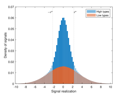
With normal signals these ex-ante distributions are also normal, with mean and variance for , so that . This implies that high-quality signals are expected to be concentrated more around the prior expectation so long as (by contrast, Proposition 1 potentially required extreme low-type variance to reach a similar conclusion). Thus, censoring to a finite radius results in a greater chance of drawing a high-type signal ( is shown here, which Figure 2 will show is optimal).
Figure 2 compares the expected utility of censoring to radius (solid line) to the expected utility of not censoring (dotted line), in all cases assuming the agent plays the optimal action given the signal received as per Equation 8. At radius , the agent is only sampling signal realizations exactly equal to the prior expectation of 0, and not learning anything. Expected utility is thus simply equal to the negative prior variance, since utility is quadratic loss. Radius maximizes the expected utility of censoring, at a level higher than the expected utility of not censoring. As goes to infinity, the expected utility with censoring approaches the expected utility with no censoring, as the radius of attention grows to encompass the full signal realization space.
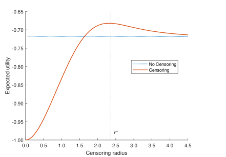
Signal realizations close to the prior expectation are more credible but less useful, since they do not lead the agent to change her beliefs much. Signal realizations far from the prior expectation are useful if true, but less credible. Figure 2 illustrates this key tradeoff: balancing credibility with usefulness. Note that this tradeoff is hard to illustrate in the binary state/signal space used in much of the literature. With a binary state, learning that someone agrees with you strengthens your trust in the accuracy of their beliefs, but is not immediately useful as it will not change your action.
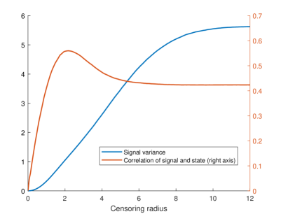
Figure 3 provides an alternative way to illustrate this tradeoff, by comparing what happens with the total variance of the signal and its correlation with the state of the world as the radius increases. Increasing increases the variance of the signal received, including valuable information about the state. Beyond the optimal radius , however, the correlation of the signal with the state diminishes as a low-type source becomes more likely.
To illustrate the conditions under which a finite sampling radius is optimal, we proceed to explore the agent’s best response in this normal framework. With normal signals, standard results in Bayesian inference yield that the optimal action given source quality is a linear convex combination of the prior expectation and the received signal. The weights are given by the relative accuracy of the prior and of the signal:
| (5) |
This linearity between the signal and the action is broken when the agent chooses a finite sampling radius , but the un-censored benchmark will nonetheless be useful to reaching the following three insights. First, conditional on the source type, the optimal action given a finite radius is more responsive to the signal than if it had come from an unbounded sampling radius. In fact, the signal is heeded more whenever the sampling radius is smaller, as Proposition 3 will show.
While the optimal action conditional on the source type is not linear, it is monotonically increasing, so is a non-linear pivot of around the prior expectation (note these policy functions necessarily intersect when ) for any and any finite .
Lemma 1.
Assume , , and are normally distributed, and . Then the optimal action is strictly increasing in the signal realization for any source type .
While Lemma 1 seems intuitive, it does rely on regularity properties afforded by the normal distribution—namely, symmetry and quasi-concavity. [60] provide clear examples illustrating why both are necessary.
Second, the ex-post belief that a signal is high quality (which determines the weights on the source-specific policy functions) is independent of the sampling radius, and monotonically decreasing in the distance between the prior expectation and the signal realization received.
Lemma 2.
If and are normal, the odds of a high-type source given a signal realization is decreasing in , independent of , and takes the following form:
Therefore, the probability of a high-type source is also decreasing in , and independent of .
Lemma 2 says that the more the signal received disagrees with the agent’s prior, the less likely it is perceived to be high-quality information. With the regularity properties of normal distributions, this is true everywhere in the signal space as long as . (Proposition 1 is similar in spirit, but requires the low-type signal noise to be high enough, and reaches a weaker conclusion.) Note that this principle can be applied to other contexts as well, such as scientific experiments. If you step on a scale and it tells you that you weigh a tenth of what you expected, most likely you need a new scale.
Lastly, the un-censored benchmark is useful because the optimal action is more responsive to the signal for any finite . In fact, the smaller the sampling radius, the more the agent heeds the signal received.
Proposition 3.
Assume , , and are normally distributed. Given a signal realization , the optimal action is decreasing in the censoring radius: .
Intuitively, a signal realization that is different from your prior expectation is more indicative of an extreme state of the world if it comes from your echo chamber than if it comes from an un-censored sample.262626Note that, from Lemma 2, we should not interpret from Proposition 3 that echo chambers make the agent more confident that the received signal comes from a high-type source; rather, it is more indicative of an extreme state. In fact, the intuition of the proof is that restricting signal realizations to a censoring radius generates a posterior belief (given signal ) that is equivalent to the posterior that would be achieved if the agent had a higher-variance prior and was drawing an un-censored signal. The effect is to put more weight on the signal and less on the prior expectation, as illustrated in Equation 5 for each source type; this effect applies to the convex combination as well, since the weights do not depend on the sampling range. In this sense, echo chambers facilitate compromise.
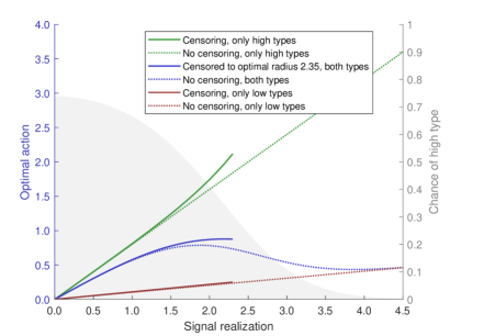
Figure 4 illustrates these pieces put together for the aforementioned parameters. The dotted blue line in the middle is the optimal action (posterior expected state) with no censoring. Per Lemma 3, this is a mixture of the optimal action with low types only and the optimal action with high types only, given by the dotted red and green lines respectively. The weight is determined by the chance of a high type for a given signal, given by the grey shading (right axis). By Lemma 2, higher signals are less likely to come from high types, so the optimal action starts off closer to the upper high-types-only ray at the origin but approaches the lower low-types-only ray as the signal goes to infinity.
The solid blue line in the middle shows the expected state if the agent samples only within the optimal radius . This is again a weighted mixture of the solid red and green lines below and above, which represent the low-types-only and high-types-only optimal actions given censoring to . Note that the agent is more responsive to signals from the echo chamber.
To sum up, in the normal framework, the optimal action is the weighted average between the response given only high types and the response given only low types. Each of these policies is a non-linear pivot of an un-censored policy which admits a simple linear closed-form. The weights on each of type-specific policy do not depend on the chosen radius,272727This property is not exclusive to normal signals—it is shown for the general framework in Appendix A2. and the weight on the high-type-only response steadily decreases as the signal gets further from the prior expectation.282828This monotonicity in the likelihood of a high type comes from the fact that the prior expected distributions of signals satisfy the monotone likelihood property—see Appendix A2 for a more general treatment Finally, the agent is more responsive to signals from smaller sampling radii.
An interesting property arising from signals with uncertain quality is that the optimal action (especially with no censoring) can exhibit non-monotonicity. Since signals further from the agent’s prior expectation are less trustworthy, they can also be less persuasive. So it may be the case that there are regions of the signal space in which the agent’s posterior belief is decreasing in the signal received—a more extreme signal results in a less extreme action.292929[97] derives a similar non-monotonicity owing to correlation in preferences.
In the normal case, the non-monotonicity occurs even though both components that are averaged, and , are monotonically increasing. The average is non-monotonic because the weights are not constant. For example in Figure 4, a signal realization of prompts a higher action than , because the agent knows that the latter almost surely came from a low-type source. In other words, a moderate view can elicit a greater response than an extreme one, because it is more trustworthy. Proposition 4 gives conditions for this non-monotonicity to occur.
Proposition 4.
Assume that the prior and signals and are distributed normally. Fix , , and . Then there exists a threshold such that implies that the optimal action without censoring is not monotonic in , and has a local maximum.
The uncertainty about the quality of a signal is key for the optimal response to be non-monotonic. So long as is in the interior, and the difference in quality between high-types and low types is big enough, the transition from an optimal response close to the high-type-only response to one close to the low-types-only response will imply some non-monotonicity. In the normal case this gap is completely dictated by the difference in variances, but non-monotonic responses can also be expected in more general settings.
Finally, with normal signals, great enough uncertainty about the signal’s quality is not only sufficient, but also a necessary condition for censoring to be optimal.
Proposition 5.
Assume , , and are distributed normally. If or , then the optimal radius is and converges to an increasing and linear function of .
The intuition of the proof is that if there is no uncertainty about the quality of information, the signal received is normal, so the posterior expected state is a linear-convex combination of the prior and the signal. The expected utility is, thus, strictly monotonic and achieves its maximum at . The continuity of the expected utility with respect to , , and completes the proof.
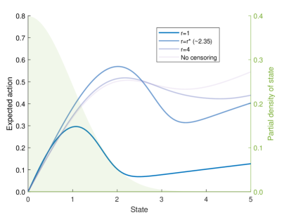
Given these results, what is the best way to disabuse the misinformed? Proposition 3 showed that echo chambers make the agent more responsive to signals, so allowing someone a signal from an echo chamber may move their beliefs further towards the truth than simply exposing them to views they don’t trust. Figure 5 plots the agent’s expected action as a function of the true state, for various censoring radii. Since the agent’s prior expectation is zero, the further the true state is from zero the more wrong the agent’s prior beliefs. While no radius dominates over all possible states, signals from the optimal echo chamber yield a greater expected response than un-censored signals for all but the most extreme states.303030If the prior expectation is very wrong (in this case, more than 2.5 standard deviations from the true state), then an un-censored signal is better ex post. But since the agent believes such a state is extremely unlikely, this is deemed a risk worth taking. So when source quality is uncertain, echo chambers may provide the best chance of correcting mistaken beliefs, since only trusted news is heeded. Note, however, that this result relies on the assumption that even within the echo chamber, signals are more likely to be close to the true state than further away.
5 Conclusion
This paper studies conditions under which echo chambers are rational. When some people’s beliefs are more accurate than others, it is reasonable to think those who agree with you are more likely to be among the well-informed (Proposition 1). So if time or attention is dear, it may be better to focus your attention on those with beliefs similar to your own (Proposition 2). As such, exposing people to contrary views may actually limit their willingness to change their own, if they have little reason to trust what they are hearing.
Importantly, this does not mean that echo chambers indicate a healthy environment for learning from others. On the contrary, they signal the presence of these two key frictions: people don’t have enough time for all the information out there, and aren’t sure who to trust. The selective exposure induced by these constraints may lead people to miss the information that would be most useful to them.
So what interventions can help? If high-quality information sources can be identified (perhaps marking the social media accounts of reporters from trusted news organizations, for example), then this would obviate the need for filtering based on signal content. Decreasing the proportion of low-quality sources (e.g. those spreading misinformation) would improve inference, though it would not preclude echo chambers—even if almost all sources are high quality, it can be preferable to focus attention on less extreme signals if the low-type signal variance is high enough (Proposition 2). Finally, improving the quality of low-type sources would reduce the incentive to filter them out. And easing the agent’s time or attention constraint would also reduce the need for filtering. However, these may be harder to translate into concrete policy recommendations.
Our work demonstrates that demand for information can differ depending on its content, not because of preferences but solely to facilitate inference. An important question not addressed here is how the supply side reacts to this phenomenon in equilibrium. Since signals closer to one’s prior expectation can elicit stronger reactions than extreme signals (Proposition 3), those seeking to persuade others with distant beliefs may find compromise more effective than accurately stating their views. However, it is not clear that such shading of signals will survive in equilibrium. Further exploration of the supply side could also entail extending the binary state space in [71] to a richer continuum to explore how consumer beliefs shape the range of views news producers313131These may include news aggregators capable of tailoring their product based on consumer characteristics—see [77]. see fit to print.
Another interesting direction might be distributional concerns in a dynamic setting. While censoring can increase the accuracy of beliefs on average, it does make those with very inaccurate priors less likely to encounter high-quality information. If the radically misinformed are unable to escape their echo chambers and suffer outsize consequences or take actions that negatively affect others, this may outweigh any benefits of accuracy that selective exposure has for others.
Our results yield a novel, testable implication: restricting someone’s ability to sample information sources based on their content can reduce the accuracy of their beliefs. Understanding the constraints that lead people to focus their attention on confirmatory views can also shed new light on existing empirical findings and provide important guidance for future work. When those in an echo chamber have less accurate beliefs than those with a more diverse diet of news (as found by e.g. [64]), one interpretation is that the echo chamber is a costly mistake. But is this difference in outcomes driven by differences in cognitive bias, or differences in constraints? Our results show that some people might choose echo chambers because they face greater constraints on time or attention. If so, exposing them to more diverse viewpoints may actually hamper their learning. Distinguishing cognitive bias from constraints on time or attention may require randomization of information sources—otherwise, different choices may simply reflect different constraints.323232[53] provide an example of such randomization. Which mechanism dominates is ultimately an empirical question, as is the degree to which beliefs are improved by selective exposure. Future work might seek to measure these forces in various contexts.
References
- [1] Daron Acemoglu, Victor Chernozhukov and Muhamet Yildiz “Fragility of asymptotic agreement under Bayesian learning” In Theoretical Economics 11.1 Wiley Online Library, 2016, pp. 187–225
- [2] Hunt Allcott and Matthew Gentzkow “Social media and fake news in the 2016 election” In Journal of Economic Perspectives 31.2 American Economic Association 2014 Broadway, Suite 305, Nashville, TN 37203-2418, 2017, pp. 211–236
- [3] Christopher A Bail “Exposure to Opposing Views can Increase Political Polarization” Harvard Dataverse, 2018 DOI: 10.7910/DVN/NSESEH
- [4] Christopher A Bail et al. “Exposure to opposing views on social media can increase political polarization” In Proceedings of the National Academy of Sciences 115.37 National Acad Sciences, 2018, pp. 9216–9221
- [5] Eytan Bakshy, Solomon Messing and Lada A Adamic “Exposure to ideologically diverse news and opinion on Facebook” In Science 348.6239 American Association for the Advancement of Science, 2015, pp. 1130–1132
- [6] Jean-Pierre Benoît and Juan Dubra “When do populations polarize? An explanation” In International Economic Review, 2019
- [7] David Blackwell “Comparison of Experiments” In Proceedings of the Second Berkeley Symposium on Mathematical Statistics and Probability Berkeley, Calif.: University of California Press, 1951, pp. 93–102 URL: https://projecteuclid.org/euclid.bsmsp/1200500222
- [8] T Renee Bowen, Danil Dmitriev and Simone Galperti “Learning from shared news: When abundant information leads to belief polarization” In The Quarterly Journal of Economics 138.2 Oxford University Press, 2023, pp. 955–1000
- [9] Paul Bromiley “Products and convolutions of Gaussian probability density functions” In Tina-Vision Memo, 2018
- [10] Randall L Calvert “The value of biased information: A rational choice model of political advice” In The Journal of Politics 47.2 Southern Political Science Association, 1985, pp. 530–555
- [11] Christopher P Chambers and Paul J Healy “Updating toward the signal” In Economic Theory 50.3 Springer, 2012, pp. 765–786
- [12] Yeon-Koo Che and Konrad Mierendorff “Optimal dynamic allocation of attention” In American Economic Review 109.8, 2019, pp. 2993–3029
- [13] Wen-Ying Sylvia Chou, April Oh and William MP Klein “Addressing health-related misinformation on social media” In Journal of the American Medical Association 320.23 American Medical Association, 2018, pp. 2417–2418
- [14] Alexander T Clark and Nicholas H Tenev “Voting and Social Pressure Under Imperfect Information” In International Economic Review 60.4 Wiley Online Library, 2019, pp. 1705–1735
- [15] J Anthony Cookson, Joseph E Engelberg and William Mullins “Echo chambers” In The Review of Financial Studies 36.2 Oxford University Press, 2023, pp. 450–500
- [16] Antonello D’agostino, Kieran McQuinn and Karl Whelan “Are some forecasters really better than others?” In Journal of Money, Credit and Banking 44.4 Wiley Online Library, 2012, pp. 715–732
- [17] Peter M DeMarzo, Dimitri Vayanos and Jeffrey Zwiebel “Persuasion bias, social influence, and unidimensional opinions” In The Quarterly Journal of Economics 118.3 MIT Press, 2003, pp. 909–968
- [18] Ester Faia, Andreas Fuster, Vincenzo Pezone and Basit Zafar “Biases in information selection and processing: Survey evidence from the pandemic” In The Review of Economics and Statistics, 2022, pp. 1–46
- [19] Peter Fischer, Eva Jonas, Dieter Frey and Stefan Schulz-Hardt “Selective exposure to information: The impact of information limits” In European Journal of Social Psychology 35.4 Wiley Online Library, 2005, pp. 469–492
- [20] Kiran Garimella, Gianmarco De Francisci Morales, Aristides Gionis and Michael Mathioudakis “Political discourse on social media: Echo chambers, gatekeepers, and the price of bipartisanship” In Proceedings of the 2018 World Wide Web Conference, 2018, pp. 913–922
- [21] Matthew Gentzkow and Jesse M Shapiro “Media bias and reputation” In NBER Working Paper, 2005
- [22] Matthew Gentzkow and Jesse M Shapiro “Media bias and reputation” In Journal of Political Economy 114.2 The University of Chicago Press, 2006, pp. 280–316
- [23] Matthew Gentzkow, Michael B Wong and Allen T Zhang “Ideological bias and trust in information sources” In Unpublished manuscript, 2021
- [24] Monica Anna Giovanniello “Echo chambers: voter-to-voter communication and political competition” In arXiv preprint arXiv:2104.04703, 2021
- [25] Russell Golman, David Hagmann and George Loewenstein “Information Avoidance” In Journal of Economic Literature 55.1, 2017, pp. 96–135 DOI: 10.1257/jel.20151245
- [26] William Hart et al. “Feeling validated versus being correct: a meta-analysis of selective exposure to information” In Psychological Bulletin 135.4 American Psychological Association, 2009, pp. 555
- [27] Seth J Hill “Learning together slowly: Bayesian learning about political facts” In The Journal of Politics 79.4 University of Chicago Press Chicago, IL, 2017, pp. 1403–1418
- [28] Lin Hu, Anqi Li and Ilya Segal “The politics of personalized news aggregation” In Journal of Political Economy Microeconomics 1.3 The University of Chicago Press Chicago, IL, 2023, pp. 463–505
- [29] Lin Hu, Anqi Li and Xu Tan “A Rational Inattention Theory of Echo Chamber” In arXiv preprint arXiv:2104.10657, 2021
- [30] Shanto Iyengar and Kyu S Hahn “Red media, blue media: Evidence of ideological selectivity in media use” In Journal of Communication 59.1 Oxford University Press, 2009, pp. 19–39
- [31] Ole Jann and Christoph Schottmüller “Why echo chambers are useful” In Oxford Department of Economics Discussion Paper, 2020
- [32] Gilat Levy and Ronny Razin “Echo chambers and their effects on economic and political outcomes” In Annual Review of Economics 11 Annual Reviews, 2019, pp. 303–328
- [33] Isaac Loh and Gregory Phelan “Dimensionality and disagreement: Asymptotic belief divergence in response to common information” In International Economic Review, 2019
- [34] George J Mailath and Larry Samuelson “Learning under Diverse World Views: Model-Based Inference” In American Economic Review 110.5, 2020, pp. 1464–1501
- [35] Delong Meng “Learning from like-minded people” In Games and Economic Behavior 126 Elsevier, 2021, pp. 231–250
- [36] Miriam J Metzger, Ethan H Hartsell and Andrew J Flanagin “Cognitive dissonance or credibility? A comparison of two theoretical explanations for selective exposure to partisan news” In Communication Research 47.1 SAGE Publications Sage CA: Los Angeles, CA, 2020, pp. 3–28
- [37] Kristoffer P Nimark and Savitar Sundaresan “Inattention and belief polarization” In Journal of Economic Theory Elsevier, 2019
- [38] Barack Obama “Farewell Address” Farewell Address of President Barack Obama, Chicago, IL, 2017 URL: https://obamawhitehouse.archives.gov/farewell
- [39] Matthew Rabin and Joel L Schrag “First impressions matter: A model of confirmatory bias” In The Quarterly Journal of Economics 114.1 MIT Press, 1999, pp. 37–82
- [40] Paola Sebastiani and Henry P Wynn “Maximum entropy sampling and optimal Bayesian experimental design” In Journal of the Royal Statistical Society: Series B (Statistical Methodology) 62.1 Wiley Online Library, 2000, pp. 145–157
- [41] Rajiv Sethi and Muhamet Yildiz “Communication with unknown perspectives” In Econometrica 84.6 Wiley Online Library, 2016, pp. 2029–2069
- [42] Ben Smith “Helping You See Outside Your Bubble” BuzzFeed, 2017 URL: https://www.buzzfeed.com/bensmith/helping-you-see-outside-your-bubble
- [43] Daniel F. Stone “Just a big misunderstanding? Bias and Bayesian affective polarization” In International Economic Review, 2019
- [44] Natalie Jomini Stroud “Selective Exposure Theories” In The Oxford Handbook of Political Communication, 2017
- [45] Wing Suen “The self-perpetuation of biased beliefs” In The Economic Journal 114.495 Oxford University Press Oxford, UK, 2004, pp. 377–396
- [46] Cass R Sunstein “# Republic: Divided democracy in the age of social media” Princeton University Press, 2018
- [47] Shiliang Tang et al. “Echo chambers in investment discussion boards” In Proceedings of the International AAAI Conference on Web and Social Media 11.1, 2017
- [48] Cole Randall Williams “Echo Chambers: Social Learning under Unobserved Heterogeneity” In The Economic Journal, 2023 DOI: 10.1093/ej/uead081
- [49] Yunhao Zhang and David G Rand “Sincere or motivated? Partisan bias in advice-taking” In Judgment and Decision Making 18, 2023, pp. e29
References
- [50] Daron Acemoglu, Victor Chernozhukov and Muhamet Yildiz “Fragility of asymptotic agreement under Bayesian learning” In Theoretical Economics 11.1 Wiley Online Library, 2016, pp. 187–225
- [51] Hunt Allcott and Matthew Gentzkow “Social media and fake news in the 2016 election” In Journal of Economic Perspectives 31.2 American Economic Association 2014 Broadway, Suite 305, Nashville, TN 37203-2418, 2017, pp. 211–236
- [52] Christopher A Bail “Exposure to Opposing Views can Increase Political Polarization” Harvard Dataverse, 2018 DOI: 10.7910/DVN/NSESEH
- [53] Christopher A Bail et al. “Exposure to opposing views on social media can increase political polarization” In Proceedings of the National Academy of Sciences 115.37 National Acad Sciences, 2018, pp. 9216–9221
- [54] Eytan Bakshy, Solomon Messing and Lada A Adamic “Exposure to ideologically diverse news and opinion on Facebook” In Science 348.6239 American Association for the Advancement of Science, 2015, pp. 1130–1132
- [55] Jean-Pierre Benoît and Juan Dubra “When do populations polarize? An explanation” In International Economic Review, 2019
- [56] David Blackwell “Comparison of Experiments” In Proceedings of the Second Berkeley Symposium on Mathematical Statistics and Probability Berkeley, Calif.: University of California Press, 1951, pp. 93–102 URL: https://projecteuclid.org/euclid.bsmsp/1200500222
- [57] T Renee Bowen, Danil Dmitriev and Simone Galperti “Learning from shared news: When abundant information leads to belief polarization” In The Quarterly Journal of Economics 138.2 Oxford University Press, 2023, pp. 955–1000
- [58] Paul Bromiley “Products and convolutions of Gaussian probability density functions” In Tina-Vision Memo, 2018
- [59] Randall L Calvert “The value of biased information: A rational choice model of political advice” In The Journal of Politics 47.2 Southern Political Science Association, 1985, pp. 530–555
- [60] Christopher P Chambers and Paul J Healy “Updating toward the signal” In Economic Theory 50.3 Springer, 2012, pp. 765–786
- [61] Yeon-Koo Che and Konrad Mierendorff “Optimal dynamic allocation of attention” In American Economic Review 109.8, 2019, pp. 2993–3029
- [62] Wen-Ying Sylvia Chou, April Oh and William MP Klein “Addressing health-related misinformation on social media” In Journal of the American Medical Association 320.23 American Medical Association, 2018, pp. 2417–2418
- [63] Alexander T Clark and Nicholas H Tenev “Voting and Social Pressure Under Imperfect Information” In International Economic Review 60.4 Wiley Online Library, 2019, pp. 1705–1735
- [64] J Anthony Cookson, Joseph E Engelberg and William Mullins “Echo chambers” In The Review of Financial Studies 36.2 Oxford University Press, 2023, pp. 450–500
- [65] Antonello D’agostino, Kieran McQuinn and Karl Whelan “Are some forecasters really better than others?” In Journal of Money, Credit and Banking 44.4 Wiley Online Library, 2012, pp. 715–732
- [66] Peter M DeMarzo, Dimitri Vayanos and Jeffrey Zwiebel “Persuasion bias, social influence, and unidimensional opinions” In The Quarterly Journal of Economics 118.3 MIT Press, 2003, pp. 909–968
- [67] Ester Faia, Andreas Fuster, Vincenzo Pezone and Basit Zafar “Biases in information selection and processing: Survey evidence from the pandemic” In The Review of Economics and Statistics, 2022, pp. 1–46
- [68] Peter Fischer, Eva Jonas, Dieter Frey and Stefan Schulz-Hardt “Selective exposure to information: The impact of information limits” In European Journal of Social Psychology 35.4 Wiley Online Library, 2005, pp. 469–492
- [69] Kiran Garimella, Gianmarco De Francisci Morales, Aristides Gionis and Michael Mathioudakis “Political discourse on social media: Echo chambers, gatekeepers, and the price of bipartisanship” In Proceedings of the 2018 World Wide Web Conference, 2018, pp. 913–922
- [70] Matthew Gentzkow and Jesse M Shapiro “Media bias and reputation” In NBER Working Paper, 2005
- [71] Matthew Gentzkow and Jesse M Shapiro “Media bias and reputation” In Journal of Political Economy 114.2 The University of Chicago Press, 2006, pp. 280–316
- [72] Matthew Gentzkow, Michael B Wong and Allen T Zhang “Ideological bias and trust in information sources” In Unpublished manuscript, 2021
- [73] Monica Anna Giovanniello “Echo chambers: voter-to-voter communication and political competition” In arXiv preprint arXiv:2104.04703, 2021
- [74] Russell Golman, David Hagmann and George Loewenstein “Information Avoidance” In Journal of Economic Literature 55.1, 2017, pp. 96–135 DOI: 10.1257/jel.20151245
- [75] William Hart et al. “Feeling validated versus being correct: a meta-analysis of selective exposure to information” In Psychological Bulletin 135.4 American Psychological Association, 2009, pp. 555
- [76] Seth J Hill “Learning together slowly: Bayesian learning about political facts” In The Journal of Politics 79.4 University of Chicago Press Chicago, IL, 2017, pp. 1403–1418
- [77] Lin Hu, Anqi Li and Ilya Segal “The politics of personalized news aggregation” In Journal of Political Economy Microeconomics 1.3 The University of Chicago Press Chicago, IL, 2023, pp. 463–505
- [78] Lin Hu, Anqi Li and Xu Tan “A Rational Inattention Theory of Echo Chamber” In arXiv preprint arXiv:2104.10657, 2021
- [79] Shanto Iyengar and Kyu S Hahn “Red media, blue media: Evidence of ideological selectivity in media use” In Journal of Communication 59.1 Oxford University Press, 2009, pp. 19–39
- [80] Ole Jann and Christoph Schottmüller “Why echo chambers are useful” In Oxford Department of Economics Discussion Paper, 2020
- [81] Gilat Levy and Ronny Razin “Echo chambers and their effects on economic and political outcomes” In Annual Review of Economics 11 Annual Reviews, 2019, pp. 303–328
- [82] Isaac Loh and Gregory Phelan “Dimensionality and disagreement: Asymptotic belief divergence in response to common information” In International Economic Review, 2019
- [83] George J Mailath and Larry Samuelson “Learning under Diverse World Views: Model-Based Inference” In American Economic Review 110.5, 2020, pp. 1464–1501
- [84] Delong Meng “Learning from like-minded people” In Games and Economic Behavior 126 Elsevier, 2021, pp. 231–250
- [85] Miriam J Metzger, Ethan H Hartsell and Andrew J Flanagin “Cognitive dissonance or credibility? A comparison of two theoretical explanations for selective exposure to partisan news” In Communication Research 47.1 SAGE Publications Sage CA: Los Angeles, CA, 2020, pp. 3–28
- [86] Kristoffer P Nimark and Savitar Sundaresan “Inattention and belief polarization” In Journal of Economic Theory Elsevier, 2019
- [87] Barack Obama “Farewell Address” Farewell Address of President Barack Obama, Chicago, IL, 2017 URL: https://obamawhitehouse.archives.gov/farewell
- [88] Matthew Rabin and Joel L Schrag “First impressions matter: A model of confirmatory bias” In The Quarterly Journal of Economics 114.1 MIT Press, 1999, pp. 37–82
- [89] Paola Sebastiani and Henry P Wynn “Maximum entropy sampling and optimal Bayesian experimental design” In Journal of the Royal Statistical Society: Series B (Statistical Methodology) 62.1 Wiley Online Library, 2000, pp. 145–157
- [90] Rajiv Sethi and Muhamet Yildiz “Communication with unknown perspectives” In Econometrica 84.6 Wiley Online Library, 2016, pp. 2029–2069
- [91] Ben Smith “Helping You See Outside Your Bubble” BuzzFeed, 2017 URL: https://www.buzzfeed.com/bensmith/helping-you-see-outside-your-bubble
- [92] Daniel F. Stone “Just a big misunderstanding? Bias and Bayesian affective polarization” In International Economic Review, 2019
- [93] Natalie Jomini Stroud “Selective Exposure Theories” In The Oxford Handbook of Political Communication, 2017
- [94] Wing Suen “The self-perpetuation of biased beliefs” In The Economic Journal 114.495 Oxford University Press Oxford, UK, 2004, pp. 377–396
- [95] Cass R Sunstein “# Republic: Divided democracy in the age of social media” Princeton University Press, 2018
- [96] Shiliang Tang et al. “Echo chambers in investment discussion boards” In Proceedings of the International AAAI Conference on Web and Social Media 11.1, 2017
- [97] Cole Randall Williams “Echo Chambers: Social Learning under Unobserved Heterogeneity” In The Economic Journal, 2023 DOI: 10.1093/ej/uead081
- [98] Yunhao Zhang and David G Rand “Sincere or motivated? Partisan bias in advice-taking” In Judgment and Decision Making 18, 2023, pp. e29
Appendix
A1 Robustness: Normal Sampling Model
This section demonstrates that the main findings are not unique to the strategy space of the main model, which requires the agent to sample signals within a radius (with equal probability) and not sample at all outside the radius. Here we consider an alternative strategy space for the agent which permits a more gradual weighting of signals distant from her prior expectation, and does not rely on sampling strategies with bounded support. Suppose that instead of choosing a censoring radius , the agent chooses a sampling function which is a normal distribution with mean and variance (Lemma 9 in Appendix A2 shows that it is optimal to choose the sampling mean equal to the prior mean regardless of the choice of variance).
For simplicity, throughout this section we also assume (as in Section 4) that the prior belief is normally distributed with mean and variance , and that the high- and low-type signal distributions are normal distributions centered on the true state with variances and , respectively. Similar to the original model (see Lemma 3 in Appendix A2), the optimal action is separable. is the convex combination of and , but each of these components is now also a convex combination of the signal and the prior expectation (Lemma 8 in Appendix A2 provides more details). That is, for , where the weight on the prior is a function of :
Lemma 2 also holds with normal sampling so long as the sampling rule does not depend on the state or the quality of the signal . If we let the optimization problem becomes
where is the distribution of signal realizations given the choice of 333333Notice that any linear transformation of generates the same signal distribution ., in particular of . The above integral admits a closed form which is best represented by defining the quality-specific weights:
and their average . With this notation at hand, the problem simplifies to:
| (6) |
where are the variances of the sampling policy conditional on type :
When the quality of information is uncertain, , and the difference in source quality is large enough, we can also have a global maximizer with (Lemma 10, Appendix A2). This complements Proposition 2 by stating the existence of other types of sampling strategies concentrated around the agent’s prior that outperform the uncensored/uniform sampling strategy whenever quality uncertainty is large enough. Moreover, similar to Proposition 5, in this setting meaningful quality uncertainty is also a necessary condition (Corollary 3, Appendix A2).
When or (equivalently) (that is, there is no quality uncertainty), all the average variables are equal to the type-specific variables, and the second term of Equation 6 vanishes. In Appendix A2, Lemma 9 shows that in this case the objective function is equal to , at , and at , the objective takes the value of with a (possible) local minimum at . In such a case, the objective does not admit an interior solution, and is maximized at , which implies uniform sampling (i.e. ).
It is not possible to rank normal vs. uniform sampling in terms of agent welfare, even for a normally distributed prior and signals—there exist cases where each is preferable. However, this section demonstrates that the main results of the paper are not an artifact of the particular sampling strategy we explored. The existence of inaccurate enough low-type sources makes weighting signals closer to one’s prior expectation preferable.
A2 Proofs and results not in the main text
[53] find that disagreement between partisans on Twitter (currently called X) increased more for a group randomly treated with incentives to follow politically opposed accounts. Using their data ([52]), Table 1 shows mean ideology (on a seven-point scale, where higher is more conservative) by initial party affiliation and treatment across the course of the study. Disagreement within the control group increased during the study (from 3.16 to 3.21), indicating the presence of forces other than treatment affecting disagreement between the parties. To be clear, our model does not generally predict increasing disagreement over time. However, it can explain why control group disagreement increased just half as much as treatment group disagreement. These results are consistent with trusted (control group) Twitter exposure having a liberal influence on the beliefs of both Democrats and Republicans, the latter of whom would otherwise have shifted to the right under the influence of other (non-Twitter) sources of news and opinion. By reducing trust in views encountered on Twitter, the treatment resulted in a greater increase in disagreement compared to the control group.
| Wave 1 | Wave 5 | ||
|---|---|---|---|
| Republicans (n=211) | 5.45 | 5.45 | |
| Control | Democrats (n=276) | 2.29 | 2.25 |
| Disagreement (R-D) | 3.16 | 3.21 | |
| Republicans (n=319) | 5.45 | 5.55 | |
| Treated | Democrats (n=416) | 2.36 | 2.35 |
| Disagreement (R-D) | 3.09 | 3.20 |
Note: Ideology measured a seven-point scale where higher is more conservative. Data from [52].
The remainder of this appendix provides further detail and results for our model, discussed in the main text. The agent’s posterior belief on the state of the world after receiving signal is:
| (7) |
Since the agent maximizes the expected value of , the optimal action given a sampling strategy equals the posterior expected state. Another way of thinking about it is that since utility is quadratic loss, maximizing utility is equivalent to minimizing the expected variance of the posterior. Given a signal realization and the sampling strategy, the optimal action is:
| (8) |
Thus, the problem of choosing reduces to the following integral
| (9) |
To study the choice of censoring policy, , we define the actions that the agent would choose if there was no uncertainty about source quality. Let
| (10) |
for source quality , where
It will be useful to note that the optimal action given a signal realization and censoring radius is separable in the following sense.
Lemma 3.
Given any censoring radius , the optimal action is a convex combination of the expected posteriors without quality uncertainty, and :
where is the posterior probability of the signal being of high quality given the signal realization received and the censoring policy, and is the chance of a low-quality source.
Proof.
The second line follows from the law of total probability, the third one from linearity of integrals, and the fourth one re-labels the variables. ∎
We now derive the unsurprising result that expected utility is higher when all signals are high-type.
Lemma 4.
The expected utility of playing with high type sources only (and no censoring) is strictly greater than that of playing with both high and low types.
Proof.
is a garbling of , since is a garbling of and for every state of the world. From [56], it follows that the value of making a decision after receiving a signal realization from is lower than making a decision after receiving a signal realization from . ∎
We now proceed with proving the results found in the main text.
Proof of Proposition 1 (in Section 3).
By Equation 1, for a given and any , . Then given , the chance of a high-type source goes to 1 as grows large:
Then we can apply this to the chance of a high-type source given a signal realization within radius :
Here , but this is not important to the result. ∎
Proof of Proposition 2 (in Section 3).
We will show that if is high enough, there exists a feasible strategy involving censoring which, while not optimal, outperforms the best expected utility achievable without censoring. Since the state has a finite variance , for any there exists such that
As , this implies
Since implies that for any ,
| (11) |
Now consider the signal . The probability distribution of given a high-type source is the product of and with mean . Since both and have finite variance, by the law of total probability does as well—denote it . Then for any there exists such that
So
Since all terms inside the integral are positive, constricting the domain of integration can only reduce it, and we have
Over the domain of integration , so this implies that
| (12) |
Letting be the maximum of and and summing inequalities 11 and 12, we have
Notice that this is equal to the expected loss (negative utility) of simply playing action conditional on a high-type source providing a signal greater than .343434Here we are taking advantage of the fact that the utility function takes the same form (quadratic) as the second moment. Were the utility function to take another functional form, we would need that the expected utility of playing be defined. The expected loss of playing optimally in this case (given by Equation 10) must be smaller, since playing is feasible. So
This shows that if is high enough and there are only high types, the contribution to overall expected utility from signals outside becomes vanishingly small. Accordingly, overall expected utility is almost unchanged if contributions from signals outside are omitted:
| (13) |
Next we show that censoring to this value of (and playing , even though it is not optimal) leaves expected utility nearly unchanged. As noted above, the probability distribution of given a high type source is the product of and . Since this distribution integrates to 1, applying this to Equation 13 means we can find high enough such that is close enough to 1 so that
| (14) |
Note that the second term on the left hand side is the expected utility of censoring to and playing (with only high types). We have thus shown that for high enough it approaches the expected utility of not censoring (again, with only high types).
By Equation 1, there exists such that for any , is arbitrarily small. Then there exists large enough that
| (15) |
Notice the proportion of high types cancels out in the second term. The interpretation is that censoring to with only high types yields nearly the same expected utility as censoring to with both types. This combined with Equation 14 shows demonstrates that there exist and high enough that
| (16) |
So as and grow, the expected utility of censoring to and playing approaches the expected utility of not censoring and playing with high types only. By Lemma 4, this exceeds the expected utility of not censoring (with both types). And the expected utility of not censoring with both types does not increase with (also by Lemma 4), and is invariant to . Thus there exist and such that censoring to provides higher expected utility than not censoring. ∎
Proof of Corollary 1 (in Section 3).
By Proposition 2, expected squared loss is lower with optimal censoring than without censoring: . Agent ’s optimal action after observing a signal drawn from radius is their posterior expectation , and by assumption it is correct in expectation: . Making these two substitutions and summing over agents yields the result: ∎
Proof of Lemma 1 (in Section 4).
We provide a more general proof, relying only on the symmetry and single-peakedness of . Let , fix , and without loss of generality let . If , then , because is symmetric about and single-peaked, so decreasing in . Accordingly, is perceived more likely given : . For states below , the reverse is true. So higher states are more likely under , and lower states are more likely under . As gets closer to , can be made arbitrarily small. So from Equation 10, we have that . ∎
Proof of Lemma 2 (in Section 4).
The odds of a high-type source are
Since both the numerator and the denominator are integrals of two Gaussian probability density functions, the product is also Gaussian with a well-known closed form. Namely,
| (17) |
for , where and are constants equal to the updated mean and variance posteriors of after observing given quality . That is,
The integral in the right hand side of equation 17 is the integral of a normal distribution, so it equals . Thus,
Rearranging terms, we obtain the result:
which is decreasing in , and therefore in as well.
∎
Lemma 5.
Fix a symmetric, quasiconcave prior state distribution and a symmetric, quasiconcave signal distribution . Then the posterior expectation after observing is greater than the prior expectation iff (“updating in the direction of the signal”— [60]).
Proof.
Without loss of generality, let have mean zero and fix . Because has mean zero,
Since is quasiconcave and symmetric about , we know that for , because . Then
| (18) |
Following the same line of argument with the inequalities reversed proves that the posterior expectation exceeds the prior only if . ∎
Lemma 6.
Fix normal prior and signal distributions and , where is the variance of .353535Since is assumed to be normal, we can think of this as signals coming from one source type only. Given a signal realization , the magnitude of the optimal action is increasing in the prior variance .
Lemma 6 says that the more diffuse an agent’s prior, the more weight is put on the signal received. We show here that this is true given normal prior and signal distributions, but this is not a necessary condition. The intuition of the proof is that starting with a sharper prior is equivalent (in terms of posterior beliefs) to starting with a more diffuse prior and receiving an additional signal equal to the prior expectation. Proposition 3 uses this lemma to show that increasing the censoring radius lowers the magnitude of the subsequent optimal action for a given signal.
Proof.
Starting from prior with mean , the posterior belief distribution after observing signal realization we will denote as , with expectation Since the prior and signal are both distributed normally, the posterior distribution is also normal, and therefore symmetric about its mean . Without loss of generality, let . By Lemma 5, this implies that the prior expectation .
Consider an alternative prior with variance . By the symmetry of about zero,
| (19) |
Because and is decreasing in , Combining this with Equation 19, we have Using , this implies The left-hand side is the posterior expectation starting from prior , and the right-hand side is (by assumption) the posterior expectation starting from the sharper prior , so this yields our result: Analogously, it can be shown in the same way that following a signal realization less than the prior expectation . ∎
Proof of Proposition 3 (in Section 4).
The intuition of the proof is that restricting signals to a censoring radius generates a posterior belief (given signal realization ) that is equivalent to the posterior generated by starting with a higher-variance prior belief and drawing an uncensored signal. The effect is to put more weight on the signal in the posterior belief.
First, consider alone. Define to be the belief distribution such that
That is, is the prior belief of state divided by the chance of a signal realization within of the prior expectation, (and then multiplied by whatever constant ensures it integrates to 1). Note that is a mean-preserving spread of : both have the same mean , but the denominator is strictly decreasing in , putting more weight on extreme states. Note also that is, like , symmetric about and decreasing as gets further from .
Observe that the posterior given censoring radius , given in Equation 7, is
In other words, the posterior belief given censoring radius and signal realization is the same as if the agent had started with the more diffuse prior belief and drawn an uncensored signal.
By Lemma 6, this implies . While is not normal, it does satisfy the essential condition ( is decreasing in ) for the lemma to hold. Following the same line of argument with instead of , we have also that .
By Lemma 3, Note that the chance of a given type does not depend on the censoring radius : and . Since both and , this yields our result: .
∎
Lemma 7 shows that with a normal prior and signals, the contribution of high-type signals to the agent’s posterior beliefs vanishes as the signal goes to infinity. This is then used to prove Proposition 4 from Section 4.
Lemma 7.
Assume , , and are distributed normally, and that . Then
| (20) |
Proof.
Since both the prior belief and the signal distribution are normal, the optimal action is a linear function of . By Lemma 2 (and for clarity, suppressing irrelevant constants), Since , a little algebra yields Then Since grows much faster than , the result follows.
∎
Proof of Proposition 4 (in Section 4).
Proof of Proposition 5 (in Section 4).
Since and are normal, they are absolutely continuous. Thus, to study the limit behavior when , or , it suffices to study the behavior at the limit. We can then assume that there is a single source, call it with variance . Equation 4 reduces to a truncated normal distribution with entropy equal to , which is monotonic in , and so is maximized at . That is, is optimal for the agent [89].
If , then Equation 4 is equal to , a normal distribution, and standard Bayesian inference yields that is a linear function of s; in fact at , . ∎
The remaining results apply to the normal sampling setup of Appendix A2.
Lemma 8.
Assume , is normal with mean and variance , and the prior belief and the signal distribution (for the unique source type) are also normally distributed with variances and , respectively. Then the signal received by the agent has distribution which is normal with mean and variance:
Proof.
The product of exponential functions is exponential and is guaranteed to be normalized appropriately to be a distribution function for each value of . See [58] for details on the calculations and the derived formulas.
∎
Lemma 9.
If , is normal with mean and variance , and the prior belief and signals are also normally distributed with mean and variances and respectively, then the optimal sampling has and .
Proof.
Given the closed form of the posterior beliefs, we have that for some policy-dependent coefficients and between zero and one that measure the relative precision of the signal received versus the prior, and of the sampling policy versus the information source:
Therefore, the optimal action is a convex combination of the signal received and the expected value of the sampling function, . Therefore, the objective function in Equation (9) has the following closed form (where is the signal distribution variance, defined by Lemma 8):
Integrating over , and using the fact that we get:
| (23) |
Here we use as shorthand for . Now, integrating over , and using the fact that ,
| (24) |
Simplifying and collecting terms, we get:
| (25) |
Since enters only in the last term of equation 25 it follows that for any given variance parameter , the utility above is maximized at , the prior expected state. Therefore, the expected utility simplifies to:
In terms of the choice variable, sampling radius , this is
| (26) |
Its unique critical point is which, if positive, is a local minimum. We conclude that no interior solution exists. Finally, we have:
Therefore the optimal policy is , which is equivalent to uniform sampling. ∎
Corollary 3.
A normal policy function with finite variance cannot outperform the uniform sampling if the variances of the two types of sources are sufficiently similar.
Proof.
When the signal variances are equal, Lemma 9 shows that uniform sampling is the optimal corner solution. By continuity, if the two variances are close enough, will be approximately normal and uniform sampling will still be optimal. ∎
Lemma 10.
If , for any and there exists threshold such that if , then .
Proof.
This proof applies the same techniques used to prove Proposition 2. In this setup we can still approximate the expected utility of receiving only high-type with arbitrary precision, if we are allowed to increase . By Lemma 8, it is possible by setting and high enough to make the distribution of high-type signals sampled by the agent arbitrarily close to the distribution of high-type signals (since ). Then, can be increased until the chance of receiving a low-type signal is arbitrarily low. Thus it is possible to set such that the agent’s expected utility is arbitrarily close to drawing uniformly from high-type signals only, as before, which by Lemma 4 exceeds the utility of setting .
∎