Optimal Design to Dual-Scale Channel Estimation for Sensing-Assisted Communication Systems
Abstract
Sensing-assisted communication is critical to enhance the system efficiency in integrated sensing and communication (ISAC) systems. However, most existing literature focuses on large-scale channel sensing, without considering the impacts of small-scale channel aging. In this paper, we investigate a dual-scale channel estimation framework for sensing-assisted communication, where both large-scale channel sensing and small-scale channel aging are considered. By modeling the channel aging effect with block fading and incorporating CRB (Cramér-Rao bound)-based sensing errors, we optimize both the time duration of large-scale detection and the frequency of small-scale update within each subframe to maximize the achievable rate while satisfying sensing requirements. Since the formulated optimization problem is non-convex, we propose a two-dimensional search-based optimization algorithm to obtain the optimal solution. Simulation results demonstrate the superiority of our proposed optimal design over three counterparts.
Index Terms:
Sensing-assisted communication, channel estimation, and channel aging.I Introduction
The ever-evolving applications of perceptive mobile network (PMN) spark the rapid evolution of ISAC[1]. But the critical spectrum conflict between sensing and communication (S&C) continues to challenge the research on more cost-effective and powerful ISAC. Enhancing integration and coordination gains of ISAC systems with minimal hardware and signal processing modifications has become a key research focus.
Sensing-assisted communication typically aims to achieve sensing-assisted beamforming, or sensing-assisted secure communication, which can further unlock the potential of ISAC systems. Radar localization can provide more accurate and direct position information than traditional channel estimation. In ISAC-enabled Vehicle-to-Everything (V2X) networks, the authors in [2] and [3] employed the state evolution model and estimated kinematic parameters for beam prediction and tracking, showing that sensing-assisted beamforming can reduce communication errors, and alleviate channel estimation overheads. Fan in [4], and Meng [5] also revealed the inverse relationship between noise offset during parameter estimation and sensing SNR, and the impact of sensing on communication is typically observed in the accuracy of angular alignment. However, most existing works overlooked the dual-scale characteristics of physical-layer channel estimation, where large-scale channel information varies slowly, but small-scale channel information varies rapidly[6]. Sensing results provide only large-scale channel information, as validated by [5], which shows that repeated sensing over short periods offers very limited improvement. Therefore, small-scale channel information should be considered to mitigate the impacts of channel aging. Although [7] and [6] analyzed the performance of ISAC systems with the dual-scale channel estimation framework from the perspectives of deep learning and compressed sampling, the analysis and optimal design that combine both the large-scale and small-scale channel information remain unexplored.
Motivated by the above discussions, this paper jointly considers and optimizes both large-scale channel detection and small-scale channel estimation in ISAC systems to maximize communication efficiency. The main contributions are summarized as follows.
-
•
We focus on dual-scale channel estimation for sensing-assisted communication systems, where we model and analyze the large-scale spatial correlation matrix based on sensing angular CRB and the small-scale channel aging, then we theoretically derive the system achievable rate. An optimal design problem is formulated to maximize the system achievable rate while satisfying the sensing requirements.
-
•
To address the non-convexity mixed integer nonlinear programming (MINLP) problem, we prove the segmented convexity of the sensing duration problem and propose a two-dimensional search-based optimization algorithm to solve it efficiently.
-
•
Simulation results demonstrate the significance and the performance improvement of our proposed design. Specifically, the proposed optimal design can improve the system achievable rate compared to three counterparts.
II System Model and Problem Formulation
We consider the downlink transmission in an ISAC system consisting of a dual-function base station (BS) and users, where BS employs a uniform linear array (ULA) with transmit antennas for communication and tracking targets, and receive antennas for the reception of sensing echo signals, and K users are denoted by .
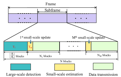
In this paper, we consider both large-scale channel detection and small-scale channel aging. As shown in Fig. 1, at the beginning of each subframe, large-scale channel detection will be conducted through a radar sensing process. The obtained large-scale spatial correlation matrix is key to efficient precoding and resource scheduling in communication systems. In addition, the small-scale Doppler shifts and the minor movement between the users and BS lead to channel aging, which makes the small-scale channel information across the transmission blocks inconsistent and time-correlated. Therefore, within a subframe, multiple small-scale channel estimations should be arranged to update the small-scale channel information such that a higher communication efficiency can be achieved. However, the increase of large-scale sensing duration and small-scale update frequency can improve the channel estimation quality but sacrifice the data transmission time. Therefore, how to optimally design the sensing duration of the large-scale channel detection and the frequency of small-scale channel update is critical and challenging in an ISAC system. In this paper, we model and analyze the impacts of dual-scale channel estimation, and propose the optimal design within specific frame structure.
II-A Frame Structure
As shown in Fig. 1, each subframe consists of blocks. The beginning of each subframe is subjected to a large-scale detection periodically, which is consistent with the design of the physical layer CSI-RS reference signals. The acquisition of large-scale slow-varying channel information is generally achieved by designing the "CSI-ResourcePeriodicityAndOffset" parameter to be periodic between 4-640 timeslots[8]. The time duration of large-scale detection is denoted as , which is an optimization variable. In addition, several small-scale estimations should be arranged at the start of some blocks (denoted as in Fig. 1, which is also an optimization variable). The time duration of small-scale estimation is fixed and denoted as . This corresponds to the design of the physical layer DM-RS and TRS reference signals[9]. Let and denote the time duration of a symbol and a block, respectively. and denote the number of symbols for each block and small-scale estimation, respectively. Then, the fixed time durations of each block and each small-scale channel estimation are and , respectively.
As shown in Fig. 1, to improve the achievable rate, this system entails a compromise on sensing duration design, i.e., the duration of large-scale detection , the number of small-scale updates , and the number of blocks for each small-scale update . Within the total blocks of each subframe, blocks are used for radar sensing to achieve large-scale channel detection, while the remaining blocks are for communication transmission.
II-B Channel Model
We assume the channel is quasi-static in each block but varies across different blocks. The classical "one-ring" model uses the spatial correlation matrix to capture large-scale information, along with the user surrounding effects of clutter. Accordingly, the time-varying channel for the user at the block can be written as [10]
| (1) |
where is the single-side angular spread, and denotes the joint angle-Doppler channel gain function on the direction of arrival (DOA) and the Doppler frequency . With the assumption that the joint angle-Doppler channel gain for different (, ) are uncorrelated, we have
| (2) |
where , and are the average channel gain, power-angle-spectrum and power-Doppler-spectrum, respectively. According to (1) and (LABEL:62615), the temporal-spatial autocorrelation matrix of is given by
| (3) |
where is the temporal correlation coefficient, and is the large-scale spatial correlation matrix111Given the temporal scope of resource scheduling spanning tens of milliseconds, it is general to assume that the large-scale characteristics of the communication channel keep constant[7]. Thus, the large-scale spatial matrix is independent of the time index.. Based on the Clarke-Jakes model[11], the temporal correlation coefficient is given by
| (4) |
where is the zeroth-order Bessel function of the first kind, and is the maximum Doppler frequency of user . Considering channel aging effects, the channel of the -th block can be characterized as
| (5) |
where is the initial channel vector derived through channel estimation. It is assumed that according to the central limit theorem (CLT)[12]. is the independent residual error.
It can be seen from (3) that both large-scale and small-scale channel estimation results influence communication efficiency. In the following subsection, we will model and analyze the large-scale channel detection and small-scale channel estimation in detail.
II-C Two-Scale Channel Estimation
II-C1 Large-Scale Detection Model
In an ISAC system, the large-scale channel detection conducted at the BS depends on the radar sensing accuracy. The sensing seudorandom sequence is transmitted as for users’ tracking at the time , where is the transmit beamforming matrix for target detection. It is assumed that the ISAC signals for different users are orthogonal, i.e., , where , and , . Accordingly, the reflected echoes at the BS is given by
| (6) |
where is the array gain factor, is the complex reflection coefficient, , and are the Doppler phase shift and time delay, respectively. stands for the complex additive white Gaussian noise at the sensing receiver. Assuming the half-wavelength antenna spacing at the BS, the transmit and receive steering vectors, i.e., , and is given by
| (7a) | |||
| (7b) | |||
Since the interference between targets is negligible in the large-scale multiple-input multiple-output (MIMO) regime and the targets can be distinguished in the delay-Doppler domain [13], the BS is capable of processing each echo signal individually, as . Thus, the output of the user after delay and Doppler frequency compensation of the matched filter is expressed as
| (8) |
where is the matched-filtering gain, is the th column of , denotes the measurement noise. Then, assuming the unbiased measurements, the angular CRB is given by[14]222Our model focuses on the impact of angular deviation on sensing, similar to [5, 4]. This is due to the consistent influence of sensing accuracy of speed, angle, and distance on resource scheduling.
| (9) |
where , and . Due to space limit, we simplify the design of , similar to [5, 11]. CRB is widely accepted as the lower bound of mean square error, we can define[15]
| (10) |
where . Since the communication channel is a function of from (1), i.e., , a first-order Taylor expansion-based delta method can be deployed to derive[16]
| (11a) | ||||
| (11b) | ||||
With (11a) and (11b), the covariance matrix of estimation error for the deterministic parameter during a single realization is . Combining with the CLT, we can conclude that
| (12) |
where is the sensing-estimated channel and is the large-scale channel error with zero mean and covariance matrix . Therefore, the large-scale correlation matrix for is given by
| (13) |
Without perfect knowledge of large-scale fading, the communication estimation on the small-scale stage should based on rather than .
II-C2 Small-scale estimation model
With the orthogonal pilot sequences of length , the observation vector for user after signal pre-processing with the imperfect large-scale information is given by [17]
| (14) |
where is the transmit power of pilot sequence, and is the time-accumulated thermal noise. Therefore, the SNR of the training sequence is typically defined as .
With the prior knowledge of the large-scale channel, the well-investigated minimum mean squared error (MMSE) estimator is given by
| (15) |
where , and the corresponding error covariance matrix of is . According to the analyses in (12) and (15), the initial channel can be represented as
| (16) |
Combined with (5), we then have
| (17) |
where is the total prediction error.
II-D Communication Rates in Dual-Scale Estimation
With the transmitted communication signal at the block , the received signals of user is given by
| (18) |
where is the Gaussian noise with mean zero and variance . , and are the interference caused by beamforming gain uncertainty and other users, respectively, and given by
|
|
(19) |
Accordingly, the signal-to-interference-plus-noise ratio (SINR) of ISAC user is given by
| (20) |
To maximize the spectral efficiency, the low-complexity maximum ratio transmission (MRT) beamforming method can be adopted as
| (21) |
where is the covariance matrix of .
Proposition 1: With the MRT transmit beamforming method in (21) and the predicted results in (17), the SINR in the n-th block is given by
| (22) |
Proof:
Please refer to Appendix A ∎
It can be seen from (22) that both small and large-scale estimations influence the communication rate. Large-scale characteristics are reflected in , while small-scale characteristics are evident in both and . The spectral efficiency (bps/Hz) in the -th block for user can be written as
| (23) |
Thus, based on the frame structure shown in Fig. 1, the system achievable rate is given by
| (24) |
where the second term at the right-hand side of (24) is the rate discount caused by the dual-scale channel estimation, and is the time duration occupied by dual-scale channel estimation.
II-E Problem Formulation
In this paper, we aim to maximize communication efficiency given in (24) while satisfying sensing requirements by jointly optimizing the large-scale sensing duration, the number of small-scale updates, and the number of blocks in each small-scale update. Thus, the optimization problem can be formulated as
| (25a) | ||||
| s. t. | (25b) | |||
| (25c) | ||||
| (25d) | ||||
| (25e) | ||||
where is the allowed maximum detection error for user ; the constraint (25b) gives the sensing requirements for each user; the constraint (25c) limits the number of communication transmission blocks to ; (25d) constraints the times of small-scale and large-scale within scheduling cycle, while (25e) constraints the number of blocks in each update not less than 1.
III Problem Decomposition and Algorithm Design
The problem is a MINLP problem that is hard to tackle. Thus, we propose the following two-dimensional search-based optimization algorithm to solve it efficiently.
III-A Determination of the number of blocks in the update (i.e., )
When and are fixed, the second row of (24) is constant and can be equivalently reformulated as
| (26a) | ||||
| s. t. | (26b) | |||
| (26c) | ||||
Since this discrete problem is intractable, we leverage the following proposition to obtain closed-form solutions.
Proposition 2: The closed-form solutions of in are given by
| (27) |
where . That is, after an even distribution equal to for each update, the remaining blocks need to spread evenly in random updates, which will have blocks, and the other updates keep to have blocks.
Proof:
Please refer to Appendix B ∎
III-B Determination of the number of small-scale updates (i.e., ) and the large-scale sensing time (i.e., )
Based on the results in (27), the achievable rate in (24) can be summarized as
With the well-known inequality , the lower bound of is given by
| (28) |
where is total transmit power of all users[11]. The channel estimation quality is reflected in , for which we have the simpler form
| (29) |
Then, the following proposition is motivated.
Proposition 3: For , when is fixed and radar’s large-scale sensing accuracy is reasonable, i.e., , the derivative of achieved throughput monotonically decreases and then it is segmented concave on .
Proof:
Please refer to Appendix C ∎
III-C Analysis of the computational complexity
According to Proposition 3, time-related resource optimization is a convex problem with fixed and blocks occupied by , i.e., . Thus, the optimal solution of this subproblem can be derived via a two-dimension search over and . For these two discrete variables, is between and , where is determined by the sensing requirements in (25b), and is between 1 and . Accordingly, there are loops and each loop optimizes a single variable via the interior-point method with complexity . The total computational complexity of the two-dimensional search-based optimization algorithm is .


IV Performance Evaluation
In this section, we evaluate the performance of our proposed optimal design. We consider an ISAC system where BS has transceivers and five users randomly distributed around it. The power budget is 23 dBm, evenly allocated to each user. All users are assumed to have the same mobility speed333Due to the space limit, we simplify the parameter setting as , users have the same speed and equal power allocation. However, the proposed analysis and method are valid in any general setting without any modifications., with block fading following , and [11]. The symbol duration us, with and (including guard interval). The scheduling cycle is 5 ms with . The sensing requirements of all users are the same, with . The power-angle-spectrum follows a uniform distribution with single-side angular spread [10].
We compare our proposed method with the following benchmark strategies: (a) Single small-scale update (SSU), which only conducts one time small-scale update at the frame’s start and optimizes the sensing duration [11]; (b) Frequent small-scale update (FSU), which performs small-scale update at each block and optimize the sensing duration [6]; (c) Random block allocation (RBA), which includes a random setting of under the dual-scale resource scheduling.
Fig. 2(a) compares the performance of achievable rate with different sensing requirements. It is observed that our proposed optimal design outperforms the three counterparts with different settings of sensing requirements. Specifically, when , our proposed method can improve the data rate by 11.3, 9.1, and 10.8 compared with SSU, FSU, and RBA, respectively. Meanwhile, it shows that the achieved rate increases with the increase of . With a larger value of , the sensing requirement is relaxed and the sensing time will minimally encroach on communication time, thus, the achieved data rate increases. It can also be seen that with a larger value of , our proposed method shows a larger performance improvement, 28.9, than SSU.
Fig. 2(b) shows the achievable rate versus the number of small-scale updates under different detection error requirements. It is observed that as increases, the achievable rate increases at first and then decreases, indicating that both too few and too frequent updates inevitably degrade the system performance. This also highlights the significance of our proposed optimal design of small-scale updates. Additionally, it can be observed that increased sensing requirements result in decreased achievable rates, due to the saturation of sensing resources encroaching on communication time.
We further demonstrate the impacts of sensing duration on the system’s achievable rate when . Note that in order to satisfy the sensing requirement, the value of sensing duration in Fig. 5 starts from 4 blocks. It is observed from Fig. 2(c) that as sensing duration increases, the achievable rate initially increases and then decreases, highlighting the trade-off between sensing and communication time. A longer sensing time improves large-scale channel accuracy but reduces communication time. Our proposed optimal design can find an optimal sensing duration to maximize communication efficiency. In addition, it is observed that the achievable rate for = 7 exceeds that for = 1 and = 20, consistent with the findings presented in Fig. 2(b) and again validates the significance of our proposed optimal design.
V Conclusion
In this paper, we have considered the dual-scale channel estimation in the sensing-assisted communication system. We have leveraged the slow-varying large-scale spatial estimation errors and fast-varying small-scale channel aging to mathematically quantify the communication rate. A joint optimization problem has been formulated to design the duration of large-scale sensing and the frequency of small-scale updates with the objective of maximizing the system achievable rate while satisfying the sensing requirements. A two-dimensional search-based algorithm has been proposed to obtain the optimal solution. Simulation results demonstrate the significance and performance improvement of the proposed method compared with the three counterparts.
Appendix A Proof of Proposition 1
Appendix B Proof of Proposition 2
The Lagrangian function of is given by
| (36) |
where is only effected by the index . To satisfy the stability condition, we require
| (37) |
Whether the optimal solution is on the boundary or not, we have the following result according to the complementary slackness condition
| (38) |
Based on the fact that , and , the rapid update of will inevitably cause a decrease in the achieved throughput. Thus, we conclude from (38). However, is a discrete variable and , which means that redundant blocks need to spread evenly in random updates. So there are updates that have blocks, and the other updates have blocks. We can conclude that
| (39) |
Appendix C Proof of Proposition 3
Based on the results in (27), the throughput in (24) can be summarized as
| (40) |
Assuming the number of blocks occupied by is fixed, will be a constant value and can be represented as , which is continuous. Therefore, only is correlated with in the first two terms of (40). Based on (28), the derivative of is given by
| (41) |
where is derived from (28). With the identity of the Neuman series for matrices[20, 21], the following approximation is given
| (42) |
therefore, we can conclude form (29) that
| (43) |
where from (11b), and is a real value since and are hermitian matrix. Since we assume , the first-order derivative of (43) on will be
| (44) |
Therefore, the maximization of is equivalent to minimizing . So, the lower bound of (43) in th iteration can be obtained by applying the first-order Taylor approximation
| (45) |
Accordingly, we can conclude
| (46) |
Since increases with , we conclude that the derivative form in (41) is monotonically decreasing with after approximation. So is concave on . For the second row of (40), combined with the in the first row, it can transformed as and its derivative is given by
| (47) |
The expressions in (47) is obviously decreases with increases, thus concave on .
References
- [1] F. Liu, Y. Cui, C. Masouros, J. Xu, T. X. Han, Y. C. Eldar, and S. Buzzi, “Integrated sensing and communications: Toward dual-functional wireless networks for 6G and beyond,” IEEE journal on selected areas in communications, vol. 40, no. 6, pp. 1728–1767, 2022.
- [2] W. Yuan, Z. Wei, S. Li, J. Yuan, and D. W. K. Ng, “Integrated sensing and communication-assisted orthogonal time frequency space transmission for vehicular networks,” IEEE Journal of Selected Topics in Signal Processing, vol. 15, no. 6, pp. 1515–1528, 2021.
- [3] F. Liu, W. Yuan, C. Masouros, and J. Yuan, “Radar-assisted predictive beamforming for vehicular links: Communication served by sensing,” IEEE Transactions on Wireless Communications, vol. 19, no. 11, pp. 7704–7719, 2020.
- [4] Y. Fan, S. Gao, D. Duan, X. Cheng, and L. Yang, “Radar integrated mimo communications for multi-hop V2V networking,” IEEE Wireless Communications Letters, vol. 12, no. 2, pp. 307–311, 2022.
- [5] K. Meng, Q. Wu, W. Chen, and D. Li, “Sensing-assisted communication in vehicular networks with intelligent surface,” IEEE Transactions on Vehicular Technology, 2023.
- [6] Z. Gao, Z. Wan, D. Zheng, S. Tan, C. Masouros, D. W. K. Ng, and S. Chen, “Integrated sensing and communication with mmWave massive mimo: A compressed sampling perspective,” IEEE Transactions on Wireless Communications, vol. 22, no. 3, pp. 1745–1762, 2022.
- [7] S. Huang, M. Zhang, Y. Gao, and Z. Feng, “MIMO radar aided mmWave time-varying channel estimation in MU-MIMO V2X communications,” IEEE Transactions on Wireless Communications, vol. 20, no. 11, pp. 7581–7594, 2021.
- [8] E. Dahlman, S. Parkvall, and J. Skold, 5G NR: The next generation wireless access technology. Academic Press, 2020.
- [9] 3GPP TS 38.221 v17.4.0,"Physical channels and modulation", 2023.
- [10] H. Li, Y. Wang, C. Sun, and Z. Wang, “Impact of channel aging on user-centric cell-free vehicular networks with non-isotropic scattering,” in Proc. IEEE Vehicular Technology Conference (VTC2023-Spring). IEEE, 2023, Florence, Italy.
- [11] J. Chen, X. Wang, and Y.-C. Liang, “Impact of channel aging on dual-function radar-communication systems: Performance analysis and resource allocation,” IEEE Transactions on Communications, vol. 71, no. 8, pp. 4972–4987, 2023.
- [12] L. You, X. Gao, A. L. Swindlehurst, and W. Zhong, “Channel acquisition for massive MIMO-OFDM with adjustable phase shift pilots,” IEEE Transactions on Signal Processing, vol. 64, no. 6, pp. 1461–1476, 2015.
- [13] H. Q. Ngo, Massive MIMO: Fundamentals and system designs. Linköping University Electronic Press, 2015.
- [14] X. Song, J. Xu, F. Liu, T. X. Han, and Y. C. Eldar, “Intelligent reflecting surface enabled sensing: Cramér-rao bound optimization,” IEEE Transactions on Signal Processing, vol. 71, pp. 2011–2026, 2023.
- [15] S. M. Kay, Fundamentals of statistical signal processing: estimation theory. Prentice-Hall, Inc., 1993.
- [16] H. Benaroya, S. M. Han, and M. Nagurka, Probability models in engineering and science. CRC press, 2005.
- [17] F. Rezaei, D. Galappaththige, C. Tellambura, and A. Maaref, “Time-spread pilot-based channel estimation for backscatter networks,” IEEE Transactions on Communications, vol. 72, pp. 434–449, 2023.
- [18] J. Zheng, J. Zhang, E. Björnson, and B. Ai, “Impact of channel aging on cell-free massive mimo over spatially correlated channels,” IEEE Transactions on Wireless Communications, vol. 20, no. 10, pp. 6451–6466, 2021.
- [19] Y. Li, C. Tao, G. Seco-Granados, A. Mezghani, A. L. Swindlehurst, and L. Liu, “Channel estimation and performance analysis of one-bit massive mimo systems,” IEEE Transactions on Signal Processing, vol. 65, no. 15, pp. 4075–4089, 2017.
- [20] K. B. Petersen, M. S. Pedersen et al., “The matrix cookbook,” Technical University of Denmark, vol. 7, no. 15, p. 510, 2008.
- [21] R. André, X. Luciani, and E. Moreau, “Joint eigenvalue decomposition algorithms based on first-order taylor expansion,” IEEE Transactions on Signal Processing, vol. 68, pp. 1716–1727, 2020.