Submitted to IEEE American Control Conference 2025
Optimal decentralized wavelength control in light sources for lithography
Abstract
Pulsed light sources are a critical component of modern lithography, with fine light beam wavelength control paramount for wafer etching accuracy. We study optimal wavelength control by casting it as a decentralized linear quadratic Gaussian (LQG) problem in presence of time-delays. In particular, we consider the multi-optics module (optics and actuators) used for generating the requisite wavelength in light sources as cooperatively interacting systems defined over a directed acyclic graph (DAG). We show that any measurement and other continuous time-delays can be exactly compensated, and the resulting optimal controller implementation at the individual optics-level outperforms any existing wavelength control techniques.
1 Introduction
The current information economy including the advent of Artificial Intelligence (AI) based generative modeling, and internet of things (IoT) has its foundations embedded in over half a century of advancements in the semiconductor industry, which has pushed the boundaries of Moore’s Law [1]. The biggest enabler of this is the photolithography process, which is currently the industry standard for manufacturing microchips. The photolithography process constitutes two main components: the wafer scanner, and a light source [2].
Wafer scanners consist of an intercombination of highly complex mechatronic systems, which combine high wafer throughput with high precision for wafer-etching. The scanning process is performed using a sequence of concatenated point-to-point motions, with the tracking specifications of the scanner’s motion systems lying in the (sub-)nanometer ranges [2, 3]. On the other hand, the light source, also known in industry as the laser, is a nonlinear, Multi-Input Multi-Output (MIMO) system. Light is generated in the form of bursts of pulses at several kHz, considered the repetition rate of the laser. These pulses illuminate a mask and expose the photo-resistive material on silicon wafers [2]. Each burst normally corresponds to one die on the wafer, and is followed by a quiescent interval, referred to as the inter-burst interval, which corresponds to moving an adjacent die into position for exposure. Since no bursts are fired in this interval, no measurements of the light are available in this period.
The three important performance specifications of the light include stability in energy, wavelength, and bandwidth, which directly impact the on chip resolution metric known as the Critical Dimension (), where represents the -factor for a given process, the wavelength, and the numerical aperture [2]. The typical values for the so-called DUV (deep ultraviolet) technology in lithography are , , and leading to line widths for ArF gas light sources [4, 5]. As such, the wavelength of the laser directly determines the size of the feature being printed. Wavelength control is achieved in modern light sources using a combination of optics that have reflective and diffractive properties, including multiple prisms, deformable mirrors, and lenses [6, 7, 3, 8, 9]. For instance, state-of-the-art DUV light sources at Cymer, LLC (an ASML company), an industry leader in light sources, have a Line Narrowing Module (LNM) that controls the light source wavelength in its Master Oscillator (MO) chamber, where the seed light is generated [10]. An LNM leverages the concepts of multiple-prism arrays and multiple-prism dispersion to control bandwidth and wavelength of a light source [11, 12]. Fig. 1 represents a schematic of multiple prisms cooperatively performing wavelength control for a light source.

In Fig. 1, light enters the LNM, and it travels through four different prisms before the diffraction grating disperses the incoming light. The directions of reflection are dependent upon the wavelength of the photons in the light beam. The wavelength in the output light is a function of the angle of incidence on the diffraction grating, prism geometry, prism refractive index, and number of prisms [12, 13]. While all four prisms have an effect on the wavelength, the prism closest to the grating (Prism ) has a larger gain from the prism angle to wavelength, followed by the previous one (Prism ) [3]. The wavelength is modified by the actuation of mechanical devices like solenoids, piezoelectric transducers (PZT), stepper motors, which are affixed to the various optics and actuate their corresponding positions/angles. For instance, Prism in Fig. 1 is driven by a stepper motor and serves as a coarse wavelength control, while the Prism is actuated by a PZT, acting as a fine wavelength control.
In this paper, we consider a two-optics module system for wavelength control for the sake of simplicity. Without loss of generality, we will assume one of the instrument is actuated by a PZT, while the other by a stepper motor. This assumption allows us to cover most of the standard actuators used for wavelength control in industry. We will use the term ‘prism’ to refer to any individual optics used for wavelength control in the remainder of the paper.
In Section 2 we review more recent work on decentralized linear quadratic Gaussian (LQG) synthesis, which form the basis for optimal cooperative wavelength control synthesis. In Section 3 we provide the problem setup for optimal decentralized wavelength control and we present our main results in Section 4. In Sections 5 and 6 we present alternate implementations, interpretations, and future work.
2 Decentralized LQG control
Dynamically decoupled decentralized systems are examples of cooperative control systems where each sub-system has independent dynamics but the sub-systems’ controllers share information via a communication topology to optimize a common, global cost. The communication network is abstracted as a directed acyclic graph (DAG). Each system is a linear time-invariant (LTI) dynamical system of the form:
| (1) | ||||
| (2) |
where and , and are the state, input, and measurement for each sub-system, and is exogenous standard Gaussian noise, independent across sub-systems and time. The infinite-horizon LQG problem is to find the causal policy that minimizes the quadratic cost is defined as
| (3) |
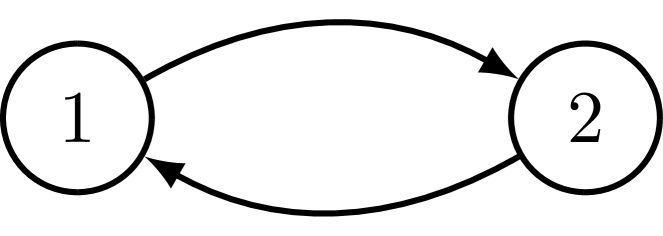
The global matrices , , , , and , obtained by stacking Eqs. 1 and 2 for each of the sub-systems, are block-diagonal in structure, and conform to the adjacency matrix of the transitive closure of the DAG. No assumptions are made on the cost matrices and , so all states and inputs may be coupled. Consider the 2-node DAG in Fig. 2.
What makes this problem decentralized is that each control signal only has access to the past history of the nodes, for which there exists a directed path from them to node . So takes the form , where the are causal maps.
In general, decentralized LQG problems are intractable, and need not have linear optimal control policies [14, 15]. However, LQG problems with partially nested information (plants and controllers structured according to a DAG) have a linear optimal control policy [16] and solving for this optimal linear controller can be cast as a convex optimization problem [17]. Explicit closed-form solutions have been obtained for decentralized linear quadratic regulator (LQR) problem using a state-space approach [18, 19] and poset-based approach [20], for LQG (output-feedback) problem [21, 18, 22, 23] and also with time delays [24, 25, 26]. These results hold for both continuous-time and discrete-time systems, and we will leverage the corresponding results to solve a continuous-time to discrete-time controller version of our problem. We present our problem setup in the next section.
3 Problem Setup
The block-diagram in Fig. 3 represents a standard prism-actuator combination in a laser. The Line Analysis Module (LAM) serves as a wavelength sensor and sampler (A/D) that converts continuous-time outputs of the system into discrete measurements. These measurements are fed into a controller that generates actuation signals for the actuator, which are converted into continuous-time signals via a Zero-Order Hold (ZOH), serving as a D/A. The PZT is modeled as a second-order system (two states) along with an integrator state for reference tracking, while the plant (prism) itself is a constant gain [27]. Analogous linear parameterization exists for a stepper motor and its corresponding gain [28, 29, 30, 31]. Note that outputs of the two systems are corresponding prism positions, while we have a single measurement; the overall wavelength. There exist DC, optics gains defined from the prism positions to wavelength: and for Prisms and respectively [3]. We define the global continuous-time system as:
| (4) | ||||
| (5) |
where are state-space matrices for the stepper, while are those of the PZT for all . The global state-vector is formed by stacking the states of the PZT, followed by the stepper. We form the global input , output , and noise in a similar manner.
3.1 Cost
The goal of the multi-prism configuration is to minimize the error () between the reference () and actual () wavelength. In reality, this wavelength error is , a combination of errors incurred from both prism positions. Without loss of generality, the cost function is defined as:
| (6) |
where is a weighting on the states of the overall system, and penalize the control signals for the PZT and the stepper respectively. The state weighting matrix is a function of the optics gains and , and allows for coupling between the states of the two sub-systems: PZT Prism , and Stepper Prism . Since the PZT is a finer actuator with a limited range, holds in practice. Note that we are considering the infinite-horizon case in this paper for simplicity, with the finite horizon cost briefly discussed in Section 5.1.
3.2 Time-delays and DAG
To the best of our knowledge, existing state-of-the-art control strategies lack communication between each other, with both prisms controlled separately in a discontinuous manner [27, 3]. However, since both prisms simultaneously control the wavelength, we establish two-way communication between the controllers as shown in Fig. 4.
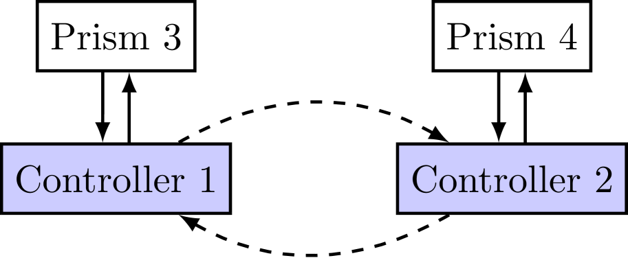
Time-delays are incurred during computation and communication of signals, named input delays, between the two sub-systems. Further there exists a measurement delay for both sub-systems due to the LAM processing. For this paper, we stick to constant delays and avoid complications associated with time-varying delays. Since the measurement delays are exactly the same for both sub-systems, we leverage the time-invariance property and commutativity with the plant to lump them together with the input delays. Thus, sub-system ’s feedback policy (in the Laplace domain) is of the form111There is no loss of generality in assuming a linear control policy [26].
| (7) |
where , , and . While the rationale for is trivial, the assumption is to satisfy the triangle inequality, i.e., information travels along the shortest path [32, 33]. Defining as the set of controllers with structure in Fig. 4 and delays in the diagonal and along cross-diagonal elements, we cast the optimal wavelength control problem as:
| (8) | ||||
where .
4 Decentralized wavelength control
Kashyap [36, Sec. 4.3] provides an explicit state-space formula for the controller and a recursive technique to handle heterogeneous delays that optimizes Eq. 8 for sub-systems. This result will be the starting point for our work. We present a modification of this result below.
Lemma 1.
[36, Thm. 43] Consider the global plant defined as , which is formed by stacking the dynamics of sub-systems, where the regulated output for cost matrices Q and R. Then the optimal in presence of heterogeneous delays by minimizing the cost is obtained by splitting the cost into N separate convex optimization problems and handling the continuous-time delays using loop-shifting. The solution of each of the N problems is for all , and are Finite Impulse Response (FIR) blocks [36, Sec. 1.5.1], and is the delay-free optimal LQG controller [37] for a rational transformation of .
The description of the infinite-dimensional FIR blocks is beyond the scope of this paper. See [36, Sec. 1.5.1] and [26, App. A] for details. We present a brief outline for deriving the optimal decentralized wavelength controller.
4.1 Solution outline
We begin with the setup in Eq. 8. Define the control cost matrix and performing Cholesky decomposition on and , we form the regulated output for wavelength control. We define the global plant
Now re-defining the cost Eq. 6 into the operator theoretic framework we obtain:
| (9) | ||||
Eq. 9 is exactly the problem setup for Lemma 1. Using the block-diagonal structure of , and , we have , which is the defining property of quadratic invariance [33]. The rest of the solution process follows the same steps as in [36, Thm. 43]. Briefly, we leverage the block-diagonal structure of to divide Eq. 9 into two smaller sub-problems. Using the loop-shifting technique [38, 39] iteratively, we compensate for , followed by in both the sub-problems. This results into two non-delayed LQG synthesis problems that are solved by standard optimal control techniques [37].
4.2 Continuous-time sub-system level controller
The solution to Eq. 8 generates an optimal controller, which can be implemented at the sub-system level. Leveraging the existing agent-level controller results for decentralized LQG problems [36, Chap. 3], we implement a continuous-time version of our controller in Fig. 5. We introduce some notation used specifically for this implementation. is a matrix of zeros with dimensions based on context of use. is an identity matrix of size . corresponds to the first columns of . Similarly is the first columns of .
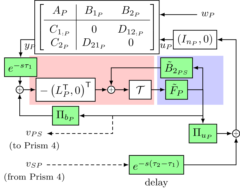
Fig. 5 represents a continuous-time implementation of the optimal controller for the PZT Prism sub-system. While the calculation of the Kalman gain remains the same as for a non-delayed, non-decentralized LQG problem, the delays alter LQR gain computations. Given a combination and if the Riccati assumptions hold [37], there is a unique stabilizing solution for
where gain , and is Hurwitz. So we evaluate the Kalman and LQR gains as and . and are modifications of , and are delay-dependent [36, 26]. The top block is a state-space matrix representation of the sub-system, which transmits wavelength measurements via the LAM. These are multiplied by the inverse of the optics gain (not shown in Fig. 5) to generate . However, we have a measurement delay incurred during this processing along-with any LAM delay, which are represented by the lumped delay term . Note that the number of states in the sub-controller is equal to the total number states of the overall system, i.e., . The Kalman filter (red) predicts the states of both the sub-systems based on available information. For the PZT Prism , the available information are . The signal already contains delayed (by s) information regarding the states of the Stepper Prism sub-system and is further delayed by a s of transmission time. The FIR blocks (feed-forward) and (feedback) together compensate for the continuous time-delays, without any Padé approximations.
5 Discussion
In this section, we consider a discrete-level implementation of the controller presented in Section 4.2 because of the pulse-by-pulse nature of the light source. A straightforward approach is to discretize the continuous-time controller, based on the sampling rate. The analog controller in Fig. 5 can be implemented as a discrete controller for a given sampling period (that satisfies the Nyquist criterion) using standard digital control emulation techniques, including bilinear transformation, matched pole-zero transform, impulse variance, ZOH, First Order Hold [40, 41, 42].
5.1 Finite horizon cost
While the controller works for a infinite horizon problem, the light sources seldom produce bursts over an infinite horizon. A finite horizon cost defined as
makes sense in such a case. The results from the infinite-horizon case are transferable. However the gains are no longer time-invariant and we can use dynamic programming approaches to solve the Hamiltonian-Jacobi-Bellman (HJB) equation associated with the differential Riccati equations to obtain and .
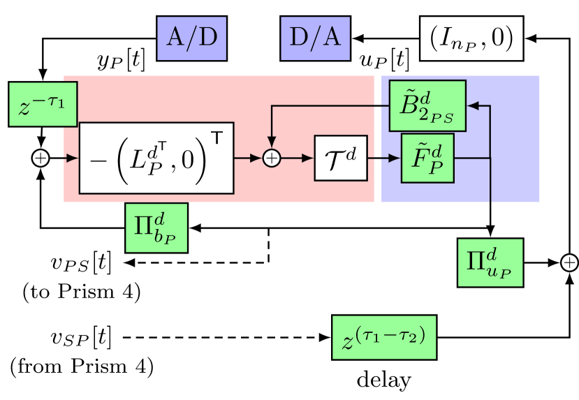
5.2 Discrete-time decentralized control
An alternate approach to the above wavelength control approach is to begin with a discretized version of the plant itself. For sampling period satisfying the Nyquist criterion, a straightforward transformation of the plant dynamics occurs: , as is non-singular, , for , with rest of the terms remaining the same. The corresponding Kalman and LQR gains are obtained by solving a discrete ARE for the infinite horizon cost case. Akin to Section 5.1, we can solve for time-varying gains using the Bellman equation for the finite-horizon cost for discrete decentralized LQG problem [43]. This approach loses the elegance and exactness of handling continuous time-delays due to the underlying approximation involved. However the structure of the discrete implementation remains similar to Fig. 5 with a discrete Kalman filter, discrete LQR, finite-dimensional FIR blocks, and time delays.
5.3 Optimality of performance
Here we show that the controller architectures provided in Figs. 5 and 6 incur the lowest cost in comparison to existing approaches for wavelength control. Current control techniques utilize a discontinuous approach, where the coarse actuator serves to desaturate the finer actuator [3]. Further the amount of wavelength target change determines whether a single actuator or a multi-actuator combination is used for control [3]. The decentralized control method allows for synchronization of the control action of both the sub-systems, ensuring a more continuous level of control. We define the average cost incurred by any sub-optimal strategies as , where is the average optimal cost for a global controller given the cost function defined in Eq. 6, and is the additional cost due to sub-optimal implementations: for instance, open-loop control of the stepper. Note that the measurement delay is already considered in this framework. Defining the cost for , we have from results in [26, Thm. 17] and [44, Lem. 9]. The final step is to establish that the cost defined for satisfies . While is implicit from [26, Thm. 17]. Using a simple limit argument and being a monotonic non-decreasing function with increasing delays [45, Prop. 6], we establish . Indeed for , and . Thus establishes the ‘optimal’ performance of the decentralized controllers in comparison to existing approaches.
5.4 Aliased disturbances
The light source open loop frequency data has several narrow-band, periodic components at known frequencies, some of which are aliased [27]. One of the primary sources of such wavelength disturbances are blowers in the gas chamber that cause acoustic waves inside the chamber, which couple into the optics [3]. For a given sampling rate, periodic disturbances can be modeled as sinusoidal signals, and this disturbance model can be integrated with the state-space formulation in Eqs. 5 and 4 as part of the PZT Prism sub-system. However, this could induce the loss of unobservability for the estimation and uncontrollability for the regulator problems in the augmented state-space system. This is not a hard constraint for solving AREs in the finite-horizon case; while workarounds exist for the infinite-horizon case. We can add a small, non-zero value to disturbance matrices for and to satisfy observability and controllability. With the prior changes, we can solve the optimal decentralized control problem for the augmented system, while simultaneously compensating for these periodic disturbances. Alternately, there exists a rich literature on implementable disturbance cancellation techniques, which are beyond the scope of this paper.
The discrete-time formulations of Figs. 5 and 6 consider a constant sampling rate. However practical considerations could require a variable sampling rate, due to laser feature specifications or the sampler characteristics. Further hardware or other restrictions could require a sampling rate different from the control rate [27]. However the elegant observer-regulator separation structure for the decentralized control problem (red-blue box separation) allows for implementation of modified Kalman filters and modified LQRs to handle these variations. It is worth noting that the LQR gain is solely delay-dependent, with only certain elements of this matrix being functions of and . This allows for faster tuning in case of time-varying delays.
6 Conclusions
We studied a practical example of a structured optimal control problem where multiple optics along-with their actuators, communicate over a delayed network for wavelength control of light in pulsed light sources. Specifically, we characterized the efficient implementation of optimal controllers at the individual optics level. We showed that these controllers incur the minimum cost compared to existing control approaches used for wavelength control in lithography. We also discussed several approaches to handle practical constraints including disturbances, intermittent sampling rates, and finite-horizon cost specifications for these controllers.
While this paper only considered the case of two prisms with their corresponding actuators, our approach is generalizable to multiple optics and actuator combinations to control wavelength in light sources used for photolithography.
References
- [1] G. E. Moore, “Cramming more components onto integrated circuits, reprinted from electronics, volume 38, number 8, april 19, 1965, pp.114 ff.” IEEE Solid-State Circuits Society Newsletter, vol. 11, no. 3, pp. 33–35, 2006.
- [2] H. Levinson, Principles of Lithography. SPIE, 2010.
- [3] M. Heertjes, H. Butler, N. Dirkx, S. van der Meulen, R. Ahlawat, K. O’Brien, J. Simonelli, K.-T. Teng, and Y. Zhao, “Control of wafer scanners: Methods and developments,” in 2020 American Control Conference (ACC), 2020, pp. 3686–3703.
- [4] R. H. French, H. Sewell, M. K. Yang, S. Peng, D. McCafferty, W. Qiu, R. C. Wheland, M. F. Lemon, L. Markoya, and M. K. Crawford, “Imaging of 32-nm 1: 1 lines and spaces using 193-nm immersion interference lithography with second-generation immersion fluids to achieve a numerical aperture of 1.5 and ak 1 of 0.25,” Journal of Micro/Nanolithography, MEMS and MOEMS, vol. 4, no. 3, pp. 031 103–031 103, 2005.
- [5] M. Rothschild and D. Ehrlich, “A review of excimer laser projection lithography,” Journal of Vacuum Science & Technology B: Microelectronics Processing and Phenomena, vol. 6, no. 1, pp. 1–17, 1988.
- [6] C. J. Chang-Hasnain, J. Harbison, C.-E. Zah, M. Maeda, L. Florez, N. Stoffel, and T.-P. Lee, “Multiple wavelength tunable surface-emitting laser arrays,” IEEE Journal of Quantum Electronics, vol. 27, no. 6, pp. 1368–1376, 1991.
- [7] L. A. Coldren, G. A. Fish, Y. Akulova, J. Barton, L. Johansson, and C. Coldren, “Tunable semiconductor lasers: A tutorial,” Journal of Lightwave Technology, vol. 22, no. 1, p. 193, 2004.
- [8] B. Mroziewicz, “External cavity wavelength tunable semiconductor lasers-a review,” Opto-Electronics Review, vol. 16, pp. 347–366, 2008.
- [9] R. Paschotta, “Ultraviolet optics,” RP Photonics Encyclopedia. [Online]. Available: https://www.rp-photonics.comultraviolet_optics.html
- [10] G. M. Blumenstock, C. Meinert, N. R. Farrar, and A. Yen, “Evolution of light source technology to support immersion and euv lithography,” in Advanced Microlithography Technologies, vol. 5645. SPIE, 2005, pp. 188–195.
- [11] I. Newton, Opticks, or, a treatise of the reflections, refractions, inflections & colours of light. Courier Corporation, 1952.
- [12] F. J. Duarte, T. S. Taylor, A. Costela, I. Garcia-Moreno, and R. Sastre, “Long-pulse narrow-linewidth dispersive solid-state dye-laser oscillator,” Applied optics, vol. 37, no. 18, pp. 3987–3989, 1998.
- [13] F. Duarte and J. Piper, “Generalized prism dispersion theory,” American Journal of Physics, vol. 51, no. 12, pp. 1132–1134, 1983.
- [14] H. S. Witsenhausen, “A counterexample in stochastic optimum control,” SIAM Journal on Control, vol. 6, no. 1, pp. 131–147, 1968.
- [15] W. Wonham, “On the separation theorem of stochastic control,” SIAM Journal on Control, vol. 6, no. 2, pp. 312–326, 1968.
- [16] Y.-C. Ho et al., “Team decision theory and information structures in optimal control problems–Part I,” IEEE Transactions on Automatic control, vol. 17, no. 1, pp. 15–22, 1972.
- [17] M. Rotkowitz and S. Lall, “Decentralized control information structures preserved under feedback,” in IEEE Conference on Decision and Control, vol. 1, 2002, pp. 569–575.
- [18] J.-H. Kim and S. Lall, “Explicit solutions to separable problems in optimal cooperative control,” IEEE Transactions on Automatic Control, vol. 60, no. 5, pp. 1304–1319, 2015.
- [19] J. Swigart and S. Lall, “Optimal controller synthesis for decentralized systems over graphs via spectral factorization,” IEEE Transactions on Automatic Control, vol. 59, no. 9, pp. 2311–2323, 2014.
- [20] P. Shah and P. A. Parrilo, “-optimal decentralized control over posets: A state-space solution for state-feedback,” IEEE Transactions on Automatic Control, vol. 58, no. 12, pp. 3084–3096, 2013.
- [21] L. Lessard and S. Lall, “Optimal control of two-player systems with output feedback,” IEEE Transactions on Automatic Control, vol. 60, no. 8, pp. 2129–2144, 2015.
- [22] T. Tanaka and P. A. Parrilo, “Optimal output feedback architecture for triangular LQG problems,” in American Control Conference, 2014, pp. 5730–5735.
- [23] M. Kashyap and L. Lessard, “Explicit agent-level optimal cooperative controllers for dynamically decoupled systems with output feedback,” in IEEE Conference on Decision and Control, 2019, pp. 8254–8259.
- [24] ——, “Agent-level optimal LQG control of dynamically decoupled systems with processing delays,” in IEEE Conference on Decision and Control, 2020, pp. 5980–5985.
- [25] A. Lamperski and L. Lessard, “Optimal decentralized state-feedback control with sparsity and delays,” Automatica, vol. 58, pp. 143–151, 2015.
- [26] M. Kashyap and L. Lessard, “Optimal control of multi-agent systems with processing delays,” IEEE Transactions on Automatic Control, pp. 1–13, 2023.
- [27] D. J. Riggs and R. R. Bitmead, “Rejection of aliased disturbances in a production pulsed light source,” IEEE Transactions on Control Systems Technology, vol. 21, no. 2, pp. 480–488, 2012.
- [28] G. McLean, “Review of recent progress in linear motors,” in IEEE Proceedings B (Electric Power Applications), vol. 135, no. 6. IET, 1988, pp. 380–416.
- [29] W. Kim, D. Shin, and C. C. Chung, “Microstepping using a disturbance observer and a variable structure controller for permanent-magnet stepper motors,” IEEE Transactions on Industrial Electronics, vol. 60, no. 7, pp. 2689–2699, 2012.
- [30] A. J. Blauch, M. Bodson, and J. Chiasson, “High-speed parameter estimation of stepper motors,” IEEE Transactions on Control Systems Technology, vol. 1, no. 4, pp. 270–279, 1993.
- [31] B. Shah, “Field oriented control of step motors,” Ph.D. dissertation, Cleveland State University, 2004.
- [32] A. Lamperski and J. C. Doyle, “The control problem for quadratically invariant systems with delays,” IEEE Transactions on Automatic Control, vol. 60, no. 7, pp. 1945–1950, 2015.
- [33] M. Rotkowitz and S. Lall, “A characterization of convex problems in decentralized control,” IEEE Transactions on Automatic Control, vol. 50, no. 12, pp. 1984–1996, 2005.
- [34] A. Lamperski and L. Lessard, “Optimal decentralized state-feedback control with sparsity and delays,” Automatica, vol. 58, pp. 143–151, 2015.
- [35] L. Lessard and S. Lall, “Convexity of decentralized controller synthesis,” IEEE Transactions on Automatic Control, vol. 61, no. 10, pp. 3122–3127, 2016.
- [36] M. Kashyap, “Optimal decentralized control with delays,” Ph.D. dissertation, Northeastern University, 2023.
- [37] K. Zhou, J. C. Doyle, and K. Glover, Robust and optimal control. Prentice-Hall, Inc., 1996.
- [38] L. Mirkin, “On the extraction of dead-time controllers and estimators from delay-free parametrizations,” IEEE Transactions on Automatic Control, vol. 48, no. 4, pp. 543–553, 2003.
- [39] L. Mirkin, Z. J. Palmor, and D. Shneiderman, “Dead-time compensation for systems with multiple i/o delays: A loop-shifting approach,” IEEE Transactions on Automatic Control, vol. 56, no. 11, pp. 2542–2554, 2011.
- [40] G. F. Franklin, J. D. Powell, M. L. Workman et al., Digital control of dynamic systems. Addison-wesley Menlo Park, 1998, vol. 3.
- [41] R. Isermann, Digital control systems. Springer Science & Business Media, 2013.
- [42] T. Chen and B. A. Francis, Optimal sampled-data control systems. Springer Science & Business Media, 2012.
- [43] A. Nayyar and L. Lessard, “Structural results for partially nested lqg systems over graphs,” in 2015 American Control Conference (ACC), 2015, pp. 5457–5464.
- [44] L. Mirkin and N. Raskin, “Every stabilizing dead-time controller has an observer–predictor-based structure,” Automatica, vol. 39, no. 10, pp. 1747–1754, 2003.
- [45] L. Mirkin, Z. Palmor, and D. Shneiderman, “ optimization for systems with adobe input delays: A loop shifting approach,” Automatica, vol. 48, no. 8, pp. 1722–1728, 2012.