Optimal consumption under a drawdown constraint over a finite horizon

Let $(\Omega,\mathcal{F},\mathbb{F},\mathbb{P})$ be a standard filtered probability space, where $\mathbb{F}=(\mathcal{F}_{t})_{t\in[0,T]}$ satisfies the usual conditions. We consider a financial market consisting of one riskless asset and one risky asset, and the terminal time horizon is denoted by $T$. The riskless asset price satisfies $dB_{t}=rB_{t}dt$ where $r\geq 0$ represents the constant interest rate. The risky asset price follows the dynamics

$$dS_{t}=S_{t}(\mu+r)dt+S_{t}\sigma dW_{t},\ \ t\in[0,T],$$

where $W$ is an $\mathbb{F}$-adapted Brownian motion and the drift $(\mu+r)$ and volatility $\sigma>0$ are given constants. It is assumed that the excessive return $\mu>0$, i.e., the risky asset’s return is higher than the interest rate.

Let $(\pi_{t})_{t\in[0,T]}$ represent the dynamic amount that the investor allocates in the risky asset and $(C_{t})_{t\in[0,T]}$ denote the dynamic consumption rate by the investor. In this paper, we consider a drawdown constraint on the excess consumption rate $c_{t}:=C_{t}-rX_{t}$ in the sense that $c_{t}$ cannot go below a fraction $\alpha\in(0,1)$ of its past maximum that

$\displaystyle c_{t}\geq\alpha z_{t},\quad t\in[0,T].$

(2.1)

Here, the non-decreasing reference process $(z_{t})_{t\in[0,T]}$ is defined as the historical excessive spending maximum

$\displaystyle z_{t}=\max\Big{\{}z,\ \sup\limits_{s\leq t}c_{s}\Big{\}},$

(2.2)

and $z\geq 0$ is the initial reference level.

In our setting, $rX_{t}$ stands for the subsistence consumption level that may refer to some mandated daily expenses in practice. On top of that, the drawdown constraint (2.1) is imposed to reflect some practical situations that some decision makers may psychologically feel painful when there is a decline in the consumption plan comparing with the past spending peak. In particular, some large expenditures not only spur some long term continuing spending such as maintenance and repair, but also lift up the investor’s standard of living that affects the future consumption decisions. Moreover, by interpreting the consumption control as dividend payment, Angoshtari et al. (2019) also discussed another motivation of the drawdown constraint that some shareholders feel disappointment when there is a decline in dividend policies.

The self-financing wealth process $X_{t}$ is then governed by the SDE that

$\displaystyle dX_{t}=(r(X_{t}-\pi_{t})-C_{t})dt+\pi_{t}\left((\mu+r)dt+\sigma dW_{t}\right),$

which can be equivalently written by

$\displaystyle dX_{t}=(\mu\pi_{t}-c_{t})dt+\sigma\pi_{t}dW_{t},\ \ t\in[0,T],$

(2.3)

with the initial wealth $X_{0}=x\geq 0$.

Let $\mathcal{A}(x)$ denote the set of admissible controls $(\pi_{t},c_{t})$ if $(\pi_{t})_{t\in[0,T]}$ is $\mathbb{F}$-progressively measurable, $(c_{t})_{t\in[0,T]}$ is $\mathbb{F}$-predictable, the integrability condition $\mathbb{E}[\int_{0}^{T}(c_{t}+\pi_{t}^{2})dt]<+\infty$ holds and the drawdown constraint $c_{t}\geq\alpha z_{t}$ is satisfied a.s. for all $t\in[0,T]$.

The goal of the agent is to maximize the expected utility of the excessive consumption rate up to time $T\wedge\tau$ under the drawdown constraint, where $\tau$ is the bankruptcy time defined by $\tau:=\inf\big{\{}t\geq 0~{}|~{}X_{t}\leq 0\big{\}}$.

To embed the control problem into a Markovian framework and facilitate the dynamic programming arguments, we choose the consumption running maximum process $z_{t}$ in (2.2) as the second state process. The value function of the stochastic control problem over a finite time horizon is given by

$\displaystyle V(x,z,t)=\sup\limits_{(\pi,c)\in\mathcal{A}(x)}\mathbb{E}\left[\int_{t}^{T\wedge\tau}e^{-\delta(s-t)}\frac{c_{s}^{1-p}}{1-p}ds+e^{-\delta(T\wedge\tau-t)}\frac{X_{T\wedge\tau}^{1-p}}{1-p}\Bigg{|}X_{t}=x,z_{t}=z\right],$

(2.4)

where the constant $\delta\geq 0$ denotes the subjective time preference parameter, and $0<p<1$ stands for the agent’s relative risk aversion coefficient.

We first note that the problem (2.4) is an extension of the control problem considered in Angoshtari et al. (2019) to the model with a finite horizon. Some new mathematical challenges arise as we encounter a parabolic variational inequality with time-dependent free boundaries. One main contribution of the present paper is that all time-dependent free boundaries stemming from the control constraint $\alpha z_{t}\leq c_{t}\leq z_{t}$ can be characterized in analytical form (see (4.13), (4.14) and (4.15) in Thereom 4.2), allowing us to identify time-dependent thresholds for the ratio between the wealth level and the past consumption running maximum to choose among different optimal feedback consumption strategies, see (2.23) in Theorem 2.1.

On the other hand, if we interpret $c_{t}$ in problem (2.4) as a control of consumption rate and regard $X_{t}$ in (2.3) as the resulting wealth process under the control pair $(\pi_{t},c_{t})$, then the control problem (2.4) is actually equivalent to a finite horizon optimal consumption problem under a drawdown constraint in the financial market with zero interest rate (as $r=0$ in the SDE (2.3) of $X_{t}$ under the control $(\pi_{t},c_{t})$). The finite horizon optimal consumption problem under a drawdown constraint has been studied by Jeon and Oh (2022), however, under the crucial assumptions that the interest rate $r>0$ and the initial wealth is sufficiently large that $X_{t}>\alpha z_{t-}\frac{1-e^{-r(T-t)}}{r}$ (see Assumption 3.1 in Jeon and Oh (2022)). Based on the martingale and duality approach, the original control problem in Jeon and Oh (2022) is transformed into an infinite series of optimal stopping problems, which requires the optimal wealth process to be strictly positive that $X_{t}>0$ and hence $X_{t}>\alpha z_{t-}\frac{1-e^{-r(T-t)}}{r}$ has to be mandated as an upper bound on $z_{t}$.

In contrast, we have interest rate $r=0$ in the equivalent optimal consumption problem, and no constraint on $X_{t}$ or $z_{t}$ is imposed because we allow the wealth process to hit zero on or before the terminal horizon $T$ and will terminate the investment and consumption control once the bankruptcy occurs. Therefore, the main results and the approach in Jeon and Oh (2022) can not cover our problem (2.4) with $r=0$ and $x\geq 0$. Instead, we rely on the technical analysis of the HJB variational inequality. Note that the interest rate $r$ does not appear in SDE (2.3) and the objective function in (2.4), our main results, especially all associated wealth thresholds, do not depend on $r$. Some major challenges are characterizing the free boundaries caused by the control constraint $\alpha z_{t}\leq c_{t}\leq z_{t}$ and the global regularity of the solution to the HJB variational inequality.

By heuristic dynamic programming arguments and the martingale optimality condition, we note that the term $\partial_{z}V=0$ holds whenever the monotone process $z_{t}$ is strictly increasing, and the associated HJB variational inequality can be written as

$$\left\{\begin{array}[]{l}\max\Big{\{}\sup\limits_{\begin{subarray}{c}\pi\in\mathbb{R},\\ \alpha z\leq c\leq z\end{subarray}}\left[\partial_{t}V+\frac{1}{2}\sigma^{2}\pi^{2}\partial_{xx}V+(\mu\pi-c)\partial_{x}V-\delta V+\frac{c^{1-p}}{1-p}\right],\partial_{z}V\Big{\}}=0,\ (x,z,t)\in Q,\\ V(0,z,t)=0,\quad\quad z>0,t\in[0,T),\\ V(x,z,T)=\frac{x^{1-p}}{1-p},\quad\quad x\geq 0,\;z>0,\end{array}\right.$$

(2.5)

where $Q:=(0,+\infty)\times(0,+\infty)\times[0,T).$

It is straightforward to see that the value function $V(x,z,t)$ in (2.4) is homogeneous of degree $1-p$ with respect to $x$ and $z$ such that $V(\beta x,\beta z,t)=\beta^{1-p}V(x,z,t)$. As a result, we can consider the change of variable

$\displaystyle\omega:=\frac{x}{z}\geq 0,$

(2.6)

and reduce the dimension that

$$V(x,z,t)=z^{1-p}V\Big{(}\frac{x}{z},1,t\Big{)}=:z^{1-p}U\Big{(}\frac{x}{z},t\Big{)}=z^{1-p}U\Big{(}\omega,t\Big{)}.$$

(2.7)

It then follows that

$\displaystyle\left\{\begin{array}[]{ll}\partial_{t}V=z^{1-p}\partial_{t}U,\\ \partial_{x}V=z^{1-p}(\frac{1}{z})\partial_{\omega}U=z^{-p}\partial_{\omega}U,\\ \partial_{xx}V=z^{-(1+p)}\partial_{\omega\omega}U,\\ \partial_{z}V=(1-p)z^{-p}U+z^{1-p}(-\frac{x}{z^{2}})\partial_{\omega}U=z^{-p}[(1-p)U-\omega\partial_{\omega}U].\end{array}\right.$

(2.12)

Moreover, let us consider the auxiliary controls $\hat{\pi}(\omega,t)=\frac{\pi(x,z,t)}{z}$ and $\hat{c}_{t}(\omega,t)=\frac{c(x,z,t)}{z}$. The HJB equation (2.5) can be rewritten as

$\displaystyle\left\{\begin{array}[]{l}\max\Big{\{}\partial_{t}U+\sup\limits_{\hat{\pi}\in\mathbb{R}}\left\{\frac{1}{2}\sigma^{2}\hat{\pi}^{2}\partial_{\omega\omega}U+\mu\hat{\pi}\partial_{\omega}U\right\}+\sup\limits_{\alpha\leq\hat{c}\leq 1}\left\{\frac{\hat{c}^{1-p}}{1-p}-\hat{c}\partial_{\omega}U\right\}-\delta U,\\ \hfill(1-p)U-\omega\partial_{\omega}U\Big{\}}=0,\quad(\omega,t)\in\mathcal{Q},\\ U(0,t)=0,\quad t\in[0,T),\\ U(\omega,T)=\frac{\omega^{1-p}}{1-p},\quad\omega\geq 0,\end{array}\right.$

(2.17)

where $\mathcal{Q}:=\mathbb{R}^{+}\times[0,T)$.

We first present the main result of the paper, and its proof is deferred to Section 4.

Based on the variational inequality (2.5) and the main results in Verification Theorem 2.1, we plot the numerical illustrations of the value function, the optimal feedback functions of portfolio and consumption in terms of the wealth variable $x$ while fixing $z=1$ and $t=0.5$ in Figure 1 as below:

As shown in Figure 1, the value function is strictly increasing and concave in the wealth variable $x$. More importantly, both optimal feedback functions of portfolio and consumption rate are increasing in $x$. However, comparing with the Merton’s solution, the optimal portfolio is no longer a constant proportion strategy of the wealth level, in fact, it is even not simply concave or convex in the wealth variable depending on the ratio of the wealth and the past consumption peak. The right-bottom panel also illustrates the piecewise consumption behavior in Theorem 2.1: when $x/z\leq\omega_{\alpha}(t)$, the optimal consumption $\hat{c}^{*}(\frac{x}{z},t)=\alpha$; when $\omega_{\alpha}(t)<x/z<\omega_{1}(t)$, the optimal consumption is the first order condition $\hat{c}^{*}(\frac{x}{z},t)=(\partial_{\omega}U)^{-\frac{1}{p}}(\frac{x}{z},t)$; and when $\omega_{1}(t)\leq x/z\leq\omega^{*}(t)$, the optimal consumption is equal to the historical consumption peak.

We plan to employ the dual transform to linearize the HJB variational inequality (2.17) and study the existence of its classical solution. To this end, we first show below that the dual transform is well defined.

As $U$ is increasing and concave in $\omega$, we can choose the candidate optimal feedback control ${\hat{\pi}}^{*}(\omega,t)$ by the first order condition that

$$\hat{\pi}^{*}(\omega,t):=-\frac{\mu}{\sigma^{2}}\frac{\partial_{\omega}U}{\partial_{\omega\omega}U}\geq 0.$$

Considering the constraint $\alpha\leq\hat{c}\leq 1$, we can choose the candidate optimal feedback control

$$\hat{c}^{*}(\omega,t):=\max\Big{\{}\alpha,\min\big{\{}1,(\partial_{\omega}U)^{-\frac{1}{p}}\big{\}}\Big{\}}.$$

(2.29)

Then (2.17) becomes

$$\left\{\begin{array}[]{l}\max\left\{\partial_{t}U-\frac{1}{2}\frac{\mu^{2}}{\sigma^{2}}\frac{(\partial_{\omega}U)^{2}}{\partial_{\omega\omega}U}+\frac{(\hat{c}^{*}(\omega,t))^{1-p}}{1-p}-{\hat{c}}^{*}(\omega,t)\partial_{\omega}U-\delta U,(1-p)U-\omega\partial_{\omega}U\right\}=0,\\ \hfill(\omega,t)\in\mathcal{Q},\\ U(0,t)=0,\quad\quad t\in[0,T),\\ U(\omega,T)=\frac{\omega^{1-p}}{1-p},\quad\omega\geq 0.\end{array}\right.$$

(2.30)

For the conjectured free boundary $\omega^{*}(t)$ in Remark 2.2 under the optimal control $(\pi^{*},c^{*})$, using the relationship between $V(x,z,t)$ and $U(\omega,t)$, $\mathcal{Q}$ can also be divided into two regions, namely the continuation region and the jump region denoted by $CR$ and $JR$ (see the illustration in Fig. 1) that

	$\displaystyle CR:=\big{\{}(\omega,t)|(1-p)U-\omega\partial_{\omega}U<0\big{\}}=\big{\{}(\omega,t)|\omega<\omega^{*}(t)\big{\}},$		(2.31)
	$\displaystyle JR:=\big{\{}(\omega,t)|(1-p)U-\omega\partial_{\omega}U=0\big{\}}=\big{\{}(\omega,t)|\omega\geq\omega^{*}(t)\big{\}}.$		(2.32)

Later, we will rigorously characterize $\omega^{*}(t)$ and two regions $CR$ and $JR$ in analytical form in Theorem 4.2.

To tackle the nonlinear parabolic variational inequality (2.30), we employ the convex dual transform that

$$u(y,t)=\max\limits_{\omega>0}[U(\omega,t)-\omega y].$$

As $\partial_{\omega\omega}(U(\omega,t)-\omega y)=\partial_{\omega\omega}U<0$, $U(\omega,t)-\omega y$ is concave in $\omega$. It implies that the critical value $\omega_{y}$ satisfies

$$\partial_{\omega}U(\omega_{y},t)=y>0.$$

(2.33)

By $\partial_{\omega\omega}U<0$, there exists $I(y,t)$, the inverse of $\partial_{\omega}U$ in $\omega$ such that

$$\omega_{y}=(\partial_{\omega}U)^{-1}(y,t)=I(y,t)>0.$$

(2.34)

Then

$$u(y,t)=U(I(y,t),t)-yI(y,t),$$

(2.35)

which leads to

	$\displaystyle\partial_{y}u(y,t)=\partial_{\omega}U(I(y,t),t)\partial_{y}I(y,t)-I(y,t)-y\partial_{y}I(y,t)=-I(y,t)<0,$		(2.36)
	$\displaystyle\partial_{yy}u(y,t)=-\partial_{y}I(y,t)=-\frac{1}{\partial_{\omega\omega}U(I(y,t),t)}>0.$		(2.37)

Hence, $I(y,t)$ strictly decreases in $y$, $u(y,t)$ strictly decreases and is convex in $y$. Moreover, it follows from (2.35) that we have

$\displaystyle\partial_{t}u(y,t)=\partial_{\omega}U(I(y,t),t)\partial_{t}I(y,t)+\partial_{t}U(I(y,t),t)-y\partial_{t}I(y,t)=\partial_{t}U(I(y,t),t).$

(2.38)

In addition, define $y_{0}(t):=\partial_{\omega}U(0,t)$, which implies that

$$\partial_{y}u(y_{0}(t),t)=-I(y_{0}(t),t)=0.$$

(2.39)

Combining (2.35) with the boundary condition (2.39), we obtain

$$u(y_{0}(t),t)=U(I(y_{0}(t),t),t)-y_{0}(t)I(y_{0}(t),t)=U(0,t)=0.$$

Therefore, we have

$$U(\omega,t)=\min\limits_{y\in(0,y_{0}(t)]}[u(y,t)+y\omega],$$

Let $y_{\omega}$ be the critical value satisfying $\partial_{y}u(y_{\omega},t)+\omega=0$, it holds that

$$U(\omega,t)=u(y_{\omega},t)+\omega y_{\omega}.$$

(2.40)

The linear dual variational inequality of (2.30) can be written as

$$\left\{\begin{array}[]{l}\max\left\{\partial_{t}u+\frac{1}{2}\frac{\mu^{2}}{\sigma^{2}}y^{2}\partial_{yy}u+\delta y\partial_{y}u-\delta u-f(y),(1-p)u+py\partial_{y}u\right\}=0,\\ \hfill(y,t)\in(0,y_{0}(t))\times(0,T],\\ u(y_{0}(t),t)=\partial_{y}u(y_{0}(t),t)=0,\\ u(y,T)=\frac{p}{1-p}y^{1-\frac{1}{p}},\quad y\geq 0,\end{array}\right.$$

(2.41)

where

$\displaystyle f(y)=\left\{\begin{array}[]{ll}\alpha y-\frac{\alpha^{1-p}}{1-p},&\mbox{if }y\geq\alpha^{-p},\\ -\frac{p}{1-p}y^{1-\frac{1}{p}},&\mbox{if }1<y<\alpha^{-p},\\ y-\frac{1}{1-p},&\mbox{if }y\leq 1,\end{array}\right.$

which is continuously differentiable in $y$. Moreover, we define $y^{*}(t)=\partial_{\omega}U(\omega^{*}(t),t)$.

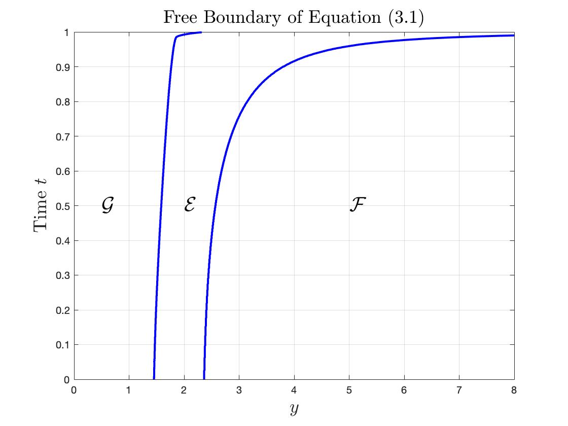
Taking advantage of the boundary condition of $u(y,t)$ on $y_{0}(t)$, we can expand the solution $u(y,t)$ to the problem (2.41) from $(0,y_{0}(t))\times(0,T]$ to the enlarged domain $\mathcal{Q}=\mathbb{R}^{+}\times[0,T)$. Let us consider $\hat{u}(y,t)$ that satisfies the auxiliary variational inequality on $\mathcal{Q}$ that

$$\left\{\begin{array}[]{l}\max\left\{\partial_{t}\hat{u}+\frac{1}{2}\frac{\mu^{2}}{\sigma^{2}}y^{2}\partial_{yy}\hat{u}+\delta y\partial_{y}\hat{u}-\delta\hat{u}-f(y),\ (1-p)\hat{u}+py\partial_{y}\hat{u},\ -\hat{u}\right\}=0,\quad(y,t)\in\mathcal{Q},\\ \hat{u}(y,T)=\frac{p}{1-p}y^{1-\frac{1}{p}},\quad y\geq 0.\end{array}\right.$$

(3.1)

It follows that

$$u(y,t)=\hat{u}(y,t),\quad(y,t)\in(0,y_{0}(t))\times(0,T].$$

For the variational inequality above, we consider the following regimes and associated free boundaries:

	$\displaystyle\mathcal{F}:=\big{\{}(y,t)\in\mathcal{Q}~{}|~{}\hat{u}(y,t)=0\big{\}}{\mbox{ (Function\ constraint region)}},$
	$\displaystyle\mathcal{G}:=\big{\{}(y,t)\in\mathcal{Q}~{}|~{}(1-p)\hat{u}(y,t)+py\partial_{y}\hat{u}(y,t)=0\big{\}}{\mbox{ (Gradient\ constraint region)}},$
	$\displaystyle\mathcal{E}:=\big{\{}(y,t)\in\mathcal{Q}~{}|~{}(1-p)\hat{u}(y,t)+py\partial_{y}\hat{u}(y,t)<0,\hat{u}(y,t)>0\big{\}}{\mbox{ (Equation region)}}.$

We plot in Figure 2 the numerical illustration of the above free boundaries as below:

To simplify some analysis, let us further set $y=e^{s}$,$\tau=T-t$ and $\tilde{u}(s,\tau)=\hat{u}(y,t)$. It follows that $\tilde{u}(s,\tau)$ satisfies

$$\left\{\begin{array}[]{l}\min\left\{\partial_{\tau}\tilde{u}-\frac{1}{2}\frac{\mu^{2}}{\sigma^{2}}\partial_{ss}\tilde{u}-(\delta-\frac{1}{2}\frac{\mu^{2}}{\sigma^{2}})\partial_{s}\tilde{u}+\delta\tilde{u}+\tilde{f}(s),\ (p-1)\tilde{u}-p\partial_{s}\tilde{u},\ \tilde{u}\right\}=0,\quad(s,\tau)\in\Omega,\\ \tilde{u}(s,0)=\frac{p}{1-p}e^{\frac{p-1}{p}s},\quad s\in\mathbb{R},\end{array}\right.$$

(3.2)

where $\Omega=(-\infty,+\infty)\times(0,T]$ and

$\displaystyle\tilde{f}(s)=\left\{\begin{array}[]{ll}\alpha e^{s}-\frac{\alpha^{1-p}}{1-p},&\mbox{if }s\geq-p\ln\alpha,\\ -\frac{p}{1-p}e^{\frac{p-1}{p}s},&\mbox{if }0<s<-p\ln\alpha,\\ e^{s}-\frac{1}{1-p},&\mbox{if }s\leq 0.\end{array}\right.$

The transformed regimes and the associated free boundaries of the variational inequality (3.2) are plotted in Figure 3 as below.

Considering

$$v(s,\tau):=e^{\frac{1-p}{p}s}\tilde{u}(s,\tau),$$

(3.4)

we can work with another auxiliary dual variational inequality of $v(s,\tau)$ that

$\displaystyle\left\{\begin{array}[]{ll}\min\left\{\partial_{\tau}v-\mathcal{L}_{s}v+e^{\frac{1-p}{p}s}\tilde{f}(s),-\partial_{s}v(s,\tau),v(s,\tau)\right\}=0,\quad(s,\tau)\in\Omega,\\ v(s,0)=\frac{p}{1-p},\quad s\in\mathbb{R},\end{array}\right.$

(3.7)

where

$$\mathcal{L}_{s}v=\frac{1}{2}\frac{\mu^{2}}{\sigma^{2}}\partial_{ss}v-\left(\frac{2-p}{2p}\frac{\mu^{2}}{\sigma^{2}}-\delta\right)\partial_{s}v-\left(\frac{1}{p}\delta-\frac{\mu^{2}(1-p)}{2p^{2}\sigma^{2}}\right)v.$$

References

- Angoshtari et al. (2019) B. Angoshtari, E. Bayraktar, and V. R. Young. Optimal dividend distribution under drawdown and ratcheting constraints on dividend rates. SIAM Journal on Financial Mathematics, 10: 547-577, 2019.
- Angoshtari et al. (2022) B. Angoshtari, E. Bayraktar, and V. R. Young. Optimal investment and consumption under a habit-formation constraint. SIAM Journal on Financial Mathematics. 13: 321-352, 2022.
- Angoshtari et al. (2023) B. Angoshtari, E. Bayraktar, and V. R. Young. Optimal consumption under a habit-formation constraint: the deterministic case. SIAM Journal on Financial Mathematics, 14:557-597, 2023.
- Arun (2012) T. Arun. The merton problem with a drawdown constraint on consumption. Preprint, available at arXiv:1210.5205, 2012.
- Bo et al. (2022) L. Bo, S. Wang, and X. Yu. A mean field game approach to equilibrium consumption under external habit formation. Stochastic Processes and their Applications, 178, 104461, 2024.
- Chen et al. (2012) X. Chen, Y. Chen, and F. Yi. Parabolic variational inequality with parameter and gradient constraints. Journal of Mathematical Analysis and Applications, 385: 928-946, 2012.
- Chen et al. (2019) X. Chen, X. Li, and F. Yi. Optimal stopping investment with non-smooth utility over an infinite time horizon. Journal of Industrial and Management Optimization, 15: 81-96, 2019.
- Chen and Yi (2012) X. Chen, and F. Yi. A problem of singular stochastic control with optimal stopping in finite horizon. SIAM Journal on Control and Optimization, 50: 2151-2172, 2012.
- Constantinides (1990) G. M. Constantinides. Habit formation: A resolution of the equity premium puzzle. Journal of Political Economy. 98(3): 519-543, 1990.
- Dai and Yi (2009) M. Dai, and F. Yi. Finite horizon optimal investment with transaction costs: A parabolic double obstacle problem. Journal of Differential Equations, 246: 1445-1469, 2009.
- Deng et al. (2022) S. Deng, X. Li, H. Pham, and X. Yu. Optimal consumption with reference to past spending maximum. Finance and Stochastics, 26: 217-266, 2022.
- Detemple and Zapatero (1992) J. Detemple, and F. Zapatero. Optimal consumption-portfolio policies with habit formation. Mathematical Finance, 2: 251-274, 1992.
- Dybvig (1995) P. H. Dybvig. Dusenberry’s racheting of consumption: optimal dynamic consumption and investment given intolerance for any decline in standard of living. Review of Economic Studies, 62: 287-313, 1995.
- Englezos and Karatzas (2009) N. Englezos, and I. Karatzas. Utility maximization with habit formation: dynamic programming and stochastic PDEs. SIAM Journal on Control and Optimization, 48: 481-520, 2009.
- Guasoni et al. (2020) P. Guasoni, G. Huberman, and D. Ren. Shortfall aversion. Mathematical Finance, 30(3): 869-920, 2020.
- Guan et al. (2019) C. Guan, F. Yi, and X. Chen. A fully nonlinear free boundary problem arising from optimal dividend and risk control model. Mathematical Control and Related Fields, 9: 425-452, 2019.
- Jeon et al. (2024) J. Jeon, T. Kim and Z. Yang. The finite-horizon retirement problem with borrowing constraint: A zero-sum stopper vs. singular-controller game. Preprint, available at SSRN: http://dx.doi.org/10.2139/ssrn.4364441.
- Jeon and Oh (2022) J. Jeon, and J. Oh. Finite horizon portfolio selection problem with a drawdown constraint on consumption. Journal of Mathematical Analysis and Applications, 506(1): 125542, 2022.
- Jeon and Park (2021) J. Jeon, and K. Park. Portfolio selection with drawdown constraint on consumption: a generalization model. Mathematical Methods of Operations Research, 93(2): 243–289, 2021.
- Li et al. (2021) X. Li, X. Yu, and Q. Zhang. Optimal consumption with loss aversion and reference to past spending maximum. SIAM Journal on Financial Mathematics, 15(1): 121-160, 2024.
- Li et al. (2022) X. Li, X. Yu, and Q. Zhang. Optimal consumption and life insurance under shortfall aversion and a drawdown constraint. Insurance: Mathematics and Economics, 108:25-45.
- Liang et al. (2022) Z. Liang, X. Luo, and F. Yuan. Consumption-investment decisions with endogenous reference point and drawdown constraint. Mathematics and Financial Economics, 17:285-334, 2023.
- Merton (1969) R. C. Merton. Lifetime portfolio selection under uncertainty: The continuous-time case. Review of Economics and Statistics, 51: 247-257, 1969.
- Merton (1971) R. C. Merton. Optimal consumption and portfolio rules in a continuous-time model. Journal of Economic Theory, 3: 373–413, 1971.
- Munk (2008) C. Munk. Portfolio and consumption choice with stochastic investment opportunities and habit formation in preferences. Journal of Economic Dynamics and Control, 32: 3560-3589, 2008.
- Protter (2005) P. E. Protter, Stochastic Integration and Differential Equations, Stoch. Model. Appl. Probab. 21, 2nd ed., Springer-Verlag, Berlin, 2005.
- Schroder and Skiadas (2002) M. Schroder, and C. Skiadas. An isomorphism between asset pricing models with and without linear habit formation. The Review of Financial Studies. 15(4): 1189-1221, 2002.
- Tanana (2021) A. Tanana. Utility maximization with ratchet and drawdown constraints on consumption in incomplete semimartingale markets. The Annals of Applied Probability, 33(5): 4127-4162, 2023.
- Yang and Yu (2022) Y. Yang, and X. Yu. Optimal entry and consumption under habit formation. Advances in Applied Probability, 54(2): 433-459, 2022.
- Yu (2015) X. Yu. Utility maximization with addictive consumption habit formation in incomplete semimartingale markets. The Annals of Applied Probability, 25(3): 1383-1419, 2015.
- Yu (2017) X. Yu. Optimal consumption under habit formation in markets with transaction costs and random endowments. The Annals of Applied Probability, 27(2): 960-1002, 2017.