Optical aberrations Correction in Postprocessing using Imaging Simulation
Abstract.
As the popularity of mobile photography continues to grow, considerable effort is being invested in the reconstruction of degraded images. Due to the spatial variation in optical aberrations, which cannot be avoided during the lens design process, recent commercial cameras have shifted some of these correction tasks from optical design to postprocessing systems. However, without engaging with the optical parameters, these systems only achieve limited correction for aberrations.
In this work, we propose a practical method for recovering the degradation caused by optical aberrations. Specifically, we establish an imaging simulation system based on our proposed optical point spread function (PSF) model. Given the optical parameters of the camera, it generates the imaging results of these specific devices. To perform the restoration, we design a spatial-adaptive network model on synthetic data pairs generated by the imaging simulation system, eliminating the overhead of capturing training data by a large amount of shooting and registration.
Moreover, we comprehensively evaluate the proposed method in simulations and experimentally with a customized digital-single-lens-reflex (DSLR) camera lens and HUAWEI HONOR 20, respectively. The experiments demonstrate that our solution successfully removes spatially variant blur and color dispersion. When compared with the state-of-the-art deblur methods, the proposed approach achieves better results with a lower computational overhead. Moreover, the reconstruction technique does not introduce artificial texture and is convenient to transfer to current commercial cameras. Project Page: https://github.com/TanGeeGo/ImagingSimulation.

Optical Aberration Correction With Imaging Simulation.
1. Introduction

Typical optical aberration degradation appearing on photos from digital cameras.
As an extension of human vision, modern digital imaging techniques have greatly enriched our methods of interacting with the world. Coupled with complex optical systems, powerful digital sensors, and heavy image signal processing (ISP) algorithms, today’s digital cameras can handle many extreme shooting scenarios, such as low-light (Chen et al., 2018), long-distance (Zhang et al., 2019) and high-dynamic-range scenarios (Yan et al., 2019; Hasinoff et al., 2016). However, sophisticated as today’s digital imaging systems are, it is difficult to totally avoid the degradation caused by optical aberration. To alleviate the aberrations while satisfying the constraints of spacing, mobile imaging devices (smartphones, DSLR cameras, etc.) adopt many different approaches. For example, the professional large aperture lens replaces ordinary glass with fluorite, and the optical stack of HUAWEI HONOR 20 has more than eight extended aspherical elements, whose aspheric coefficients are up to order 16 (Zhenggang, 2016).
In addition to the optical lens module, ISP algorithms also make a large difference in optical aberration correction. However, as shown in Figure 2a and Figure 2b, the blur and chromatic dispersion vary greatly when the optical system changes. Moreover, the current classical ISP systems still cannot handle these issues completely, therefore introducing the ”ringing effect” (see Figure 2c). These defects are very common in high-contrast photos from many recent flagship devices.
Over the past decade, methods based on the deep learning model have been evolving rapidly and have the potential to replace conventional ISP systems (Ignatov et al., 2020). The classical postprocessing system is a step-by-step process. The optical aberrations of lens and the error of noise diagnosis will accumulate and be amplified in the subsequent white balance (WB), color correction matrix (CCM), gamma operations, and so on. (Heide et al., 2014). Nevertheless, end-to-end deep learning methods do not suffer from this problem (Abdelhamed et al., 2018). Although deep learning networks allow us to restore latent images from degraded images, the learned models always achieve unsatisfactory results when evaluating real data (Cai et al., 2020). Therefore, generating targeted datasets that follow the distribution of real scenes is the principal part of the deep learning method (Ji et al., 2020). In recent years, many scholars have gained insight into this field. Their proposed approaches are characterized by a considerable amount of shooting and alignment (Ignatov et al., 2017). However, a large quantity of training data is required to prevent overfitting, which conversely exacerbates the workload (Peng et al., 2019). Furthermore, because each imaging system exhibits entirely different characteristics, adapting a CNN-based algorithm to a new camera may require capturing many new data pairs (Ignatov and Timofte, 2019). Therefore, it is imperative to design a brand new method for dataset generation that combines optical parameters and is easy to transfer to other cameras.
In this work, we propose a practical method for recovering the degradation caused by optical aberrations. To achieve this, we establish an imaging simulation system based on raytracing and coherent superposition (Paul, 2014). Given the lens data and parameters of the sensor, it works out the imaging result of a definite object at a fixed distance. With datasets established by the imaging simulation system, we design a postprocessing chain, which combines field-of-view (FOV) information and optical parameters to perform adaptive restoration on the degraded data (Heide et al., 2014). The proposed method outperforms many state-of-the-art deblurring methods on synthetic data pairs, as does the evaluation. When evaluated on real images, our proposed technique achieves better visual results and requires lower computational overhead. Moreover, our approach is convenient for transferring to other commercial lenses, and there are no limitations on the optical design.
Our main technical contributions are as follows:
-
•
An optical point spread function model is proposed for accurate PSF calculation in a simulation manner.
-
•
Based on the ISP algorithms, an imaging simulation system is established. Given the camera’s optical parameters, it generates targeted data pairs following the distribution of lens optical aberrations.
-
•
A novel spatial-adaptive CNN architecture is proposed, which introduces FOV input, deformable ResBlock, and context block to adapt to spatially variant degradation.
This paper proceeds as follows. In Section 2, we review the related works. In Section 3, we present an overview of our methods. In Section 4, we detail the proposed optical PSF model and the composition of the imaging simulation system. In Section 5 and Section 6, we present a brand new postprocessing pipeline. In Section 7, we compare our approach’s improved performance with the state-of-the-art methods and perform an ablation study on each aspect of our approach. In Section 8, we assess the proposed approach and demonstrate its potential applications.
2. Related Work
Optical Aberration. According to Fermat’s principle, rays of light traverse the path of stationary optical path length with respect to variations in the path (Westphal et al., 2002). Therefore, when the incident angle of rays changes, so does the optical length (Smith, 2005). Generally, the distinction of optical length manifests as weird blur and pixel displacement, which becomes more severe with increasing numerical aperture and FOV (Smith, 2008). While limited by the requirements of physical space, optical parameters, and machining tolerance, it is difficult for classical lens design to suppress optical aberrations (Sliusarev, 1984).
Point Spread Function Model. A large body of work in this field has proposed calibrating and measuring PSFs from a single image (Hirsch and Scholkopf, 2015; Shih et al., 2012; Jemec et al., 2017; Ahi, 2017). These methods often estimate optical blur functions or chromatic aberrations either blindly or through a calibration process. Moreover, recent works propose developing a machine learning framework to estimate the underlying physical PSF model from the given camera lens (Herbel et al., 2018). However, these approaches have several limitations in operation, such as the noise level and the field interval of calibration or estimation (Heide et al., 2013). The closest related works to us are those approaches that compute PSFs with lens prescriptions (Shih et al., 2012). Given the focal length, aperture, focusing distance, and white balance information, these methods simulate the image plane PSFs of each virtual object point.
Unfortunately, the PSFs calculated by their method are different from the measured PSFs (after ISP). The reasons for mismatching are summarized as manufacturing tolerances and fabrication errors during lens production (Shih et al., 2012). However, we hold different views from them. We believe that the PSFs calculated by lens prescription represent the diffusion of energy, which are essentially different from the measured PSFs after ISP. (Paulin-Henriksson et al., 2008). And the complex amplitude of each ray must be considered while calculating the PSFs. Therefore, coherent superposition must be conducted after raytracing. To make a comprehensive comparison to prove the accuracy of the computed energy PSFs, we apply the calculated PSFs to the checkerboard chart in the energy domain and then transform the degraded image to a visualized image. The similarity of the real images and the synthetic results illustrates that it is a practical method for simulating PSFs with the advantages of lens prescriptions if the process of imaging is properly modeled.
Image Reconstruction. The optical aberration correction of a real image can be regarded as a problem of image reconstruction, where the goals are to increase sharpness and restore detailed features of images. Traditional deconvolution methods (Heide et al., 2013; Pan et al., 2016; Sun et al., 2017) use various natural image priors for iterative and mutual optimization, which unfortunately are not robust and have poor computational efficiency when handling large spatially variant blur kernels. The point spread functions of large FOV lenses vary from 11 to 53 pixels, which presents a great challenge to existing deconvolution methods, necessitating a custom image reconstruction approach. In recent years, a large number of efficient solutions have been proposed to use deep learning models for image processing tasks (Schuler et al., 2016; Agustsson and Timofte, 2017; Nah et al., 2017; Vedaldi and Fulkerson, 2010), starting from the simplest CNN approaches (Sun et al., 2015; Dong et al., 2016; Kim et al., 2016; Shi et al., 2016), to deep residual and attention models (Zhang et al., 2019; Wang et al., 2019; Ratnasingam, 2019) and complex generative adversarial networks (GANs) (Ledig et al., 2017; Sajjadi et al., 2017; Wang et al., 2018; Ignatov et al., 2020). More recently, (Peng et al., 2019) proposed a learned generative reconstruction model, a single deep Fresnel lens design tailored to this model, obtaining pleasant results.
All of these approaches have in common that they require either accurate PSF estimation (Heide et al., 2013) or large training data that have been manually acquired (Ignatov et al., 2020). Moreover, when the lens design changes, painful acquisition is still needed to obtain targeted image pairs, which include shooting, registration, and color correction (Peng et al., 2019). In contrast, our proposed imaging simulation system generates a large number of training corpora with encoded optical information. Moreover, our approach is practical and easy to transfer to other lens designs. Our network model combines the optical parameters and FOV information, allowing us to efficiently address the large scene-dependent blur and color shift of commercial lens design.
Mobile Image Signal Processing. There exist many classical approaches for various image signal processing subtasks, such as image demosaicing (Hirakawa and Parks, 2005; Dubois, 2006; Li et al., 2008), denoising (Buades et al., 2005; Foi et al., 2008; Condat, 2010; Chang et al., 2020), white balancing (Schwartzburg et al., 2014; van de Weijer et al., 2007; Gijsenij et al., 2012), and color correction (Kwok et al., 2013). Only a few works have explored the applicability of combining optical parameters with imaging signal processing systems. Recently, some deep learning methods were proposed to map low-quality smartphone RGB/RAW photos to superior-quality images obtained with a high-end reflex camera (Ignatov et al., 2017). The collected datasets were later used in many subsequent works (Ignatov et al., 2018; Ignatov et al., 2020; Mei et al., 2019), which achieved significantly improved results. Additionally, in (Agustsson and Timofte, 2017; Ignatov and Timofte, 2019), the authors examined the possibility of running image enhancement models directly on smartphones and proposed several efficient solutions for this task.
It is worth mentioning that all these datasets’ construction methods require a considerable amount of shooting and registration. Moreover, owing to the different perspectives of data pairs, the resulting image enhancement model will introduce a small displacement to the input data, which is different from lens distortion correction. Additionally, these methods map the degradation images shot by a poor imaging system to the photos shot by a better imaging system; in other words, the upper bound of recovery depends on the quality of the ground truth. In contrast, the quality of the ground truth is also important but not critical to our method, because we encode the optical aberration degradation in the PSFs instead of the image pairs. And our approach generates data in a simulation manner, which liberates us from many duplicate acquisitions.
3. Overview

Overview.
The goal of our work is to propose a practical method for recovering the degradation caused by optical aberrations. To achieve this, we engage optical parameters with a brand new postprocessing chain (as shown in Figure 3.b). The two core ideas behind the proposed method are as follows: first, to eliminate the blurring, displacement, and chromatic aberrations caused by lens design, we design a spatially adaptive network architecture and insert it into the postprocessing chain. Second, for the sake of portability, we design an imaging simulation system for dataset generation, which simulates the imaging results of a specific camera and generates a large training corpus for deep learning methods.
Therefore, we rely on the proposed optical PSF model to establish the imaging simulation system. Different from the traditional raytracing or fast Fourier transform (FFT) methods to calculate PSF, we regard each ray as a secondary light source. The complex amplitude of each ray is superposed on the image plane; therefore, the PSF is the intensity of complex amplitude after superposition. In this way, the proposed method determines the degenerative consequences of object points. Figure 8 shows the spatially variant point spread functions of the customized DSLR camera lens and HUAWEI HONOR 20, which are computed following our optical PSF model. After calculating the PSFs of the lens, we establish an imaging simulation system based on the ISP pipeline of the digital camera. The simulation pipeline is detailed in Figure 5. To the best of our knowledge, we are the first to generate datasets of optical aberrations in a simulation manner, which do not need a great deal of shooting, registration, and color correction. We emphasize that our simulation method is easy to transfer to other lenses and has no limitations on optical designs.
Because of the spatially variant characteristics of optical aberrations, we design a brand new spatial-adaptive network architecture that takes the degraded image and FOV information as the input to directly reconstruct the aberration-free image. Together with the datasets generated by the imaging simulation system and the newly proposed postprocessing chain (Figure 3.b), we can address the spectral and FOV-dependent blurring, color shift, and sharpness loss caused by lens aberrations.
4. Imaging Simulation System
In this section, we start by introducing the proposed optical PSF model, which consists of raytracing and coherent superposition. Second, we illustrate the relative illumination distribution and sensor spectral response calculation, which are used to connect the separate PSFs of different wavelengths to the accurate energy PSFs. Third, based on the ISP systems of modern digital cameras, we design an imaging simulation pipeline (Figure 5), which is applied to the input images, and generate the results degraded by PSFs depending on the spectral distribution and FOV information.
4.1. Optical PSF Model
For photographic objective systems with large FOVs and apertures, it is inaccurate to derive the PSF analytic solution by Gaussian paraxial approximation (Born and Wolf, 2013) or fast Fourier transform (FFT) (Manual, 2009) (we recommend readers to supplementary materials for relevant information). In other words, for various commercial optical designs, sequential raytracing and coherent superposition are the only universal methods to obtain precise point spread functions on the imaging plane.
In the image formation process, every point of the object can be regarded as a coherent light source . For a particular light source , a grid of rays is launched through the optical system, which forms the wavefront at the exit pupil. According to the Huygens principle, every point on a wavefront is the source of spherical wavelets, and the secondary wavelets emanating from different points mutually interfere (Baker and Copson, 2003; Paul, 2014). In other words, the diffraction intensity at any point on the image plane is the complex sum of all these wavelets, squared. Therefore, in our proposed optical PSF model, the PSF on the image grid is computed in two stages, the first stage uses the sequential raytracing method to compute the wavefront distribution at the exit pupil plane, and the second stage uses coherent superposition to output the PSF calculation.
4.1.1. Raytracing
The skew ray emitted by a coherent monochromatic light source is a perfectly general ray, which can be defined by the starting point O = (, , ) of , and by its normalized direction vector D = (, , ). We can express the ray P = (, , ) in parametric form, where is the ray marching distance:
| (1) |
After defining a general ray, raytracing can be divided into two steps: The first step is to calculate the intersection point of light and the surface. The surface equation generally used in optical design can be formulated as follows:
| (2) |
where is the longitudinal coordinate of a point on the surface, and is the distance from the point to axis. is the curvature of the spherical part. The subsequent terms represent deformations to the spherical part, with , , , as the constant of the second, fourth, ., power deformation terms.
We build the simultaneous equations of Eq. 1 and Eq. 2 for solving the ray marching distance from the starting point O to the next ray-surface intersection point. However, their solution cannot be directly determined by the higher-order equations. Therefore, our raytracing is accomplished by a series of approximations. In each approximation, we add a small increment to the ray marching distance and compute P = (, , ) with Eq.1 to obtain the coordinates of ray. Additionally, we substitute and into Eq. 2 to acquire the , which is the longitudinal coordinate of the surface. The iteration is repeated until the disparity between and is negligible. In this way, the intersection of light and the surface is computed.
The second step is to calculate the refraction of light on the medium surface. Following Snell’s law, the refracted angle can be computed by:
| (3) |
Here, n is the normal unit vector of the surface equation, and and are the refractive indexes on both sides of the surface. is the operation of computing the cosine value of two vectors. In this way, the refracted direction vector D’ can be calculated by:
| (4) |
In the implementation, we perform sequential raytracing for every sample position on the pupil plane. The direction vector and the total optical path length are recorded. We note that every object point can be regarded as a coherent light source , so the diffusion of energy is the superposition result of the coherent wavelet (as demonstrated in Section. 4.1). In the following section, we introduce the details of coherent superposition.
4.1.2. coherent superposition

Coherent Superposition.
After tracing a grid of rays that is uniformly sampled on the pupil, we obtain the wavefront distribution at the exit pupil plane. Figure 4 shows the wavefront distribution of converging light at the virtual exit pupil plane. We note that each ray of this wavefront distribution represents a spherical wavelet with a particular amplitude and phase, so the complex amplitude of Huygens’ wavelet in the pupil plane can be represented by:
| (5) |
where is the length of total optical path from to , where and are the spatial coordinates of the pupil plane. is the amplitude of the spherical wave at the unit distance from the source. is the wave number of the light.
The complex amplitude propagating to the image plane can be formulated as follows:
| (6) |
where the , and is the obliquity factor of the spherical wavelet, which is defined as follows:
| (7) |
where is the normal unit vector of the exit pupil plane and is the operation of computing the cosine value of the two vectors. The relationships of , , and are magnified in Figure 4.
Therefore, the complex amplitude at the point on the image surface is the complex sum of all the wavefront distributions propagated from the exit pupil plane, which can be formulated as the following equation:
| (8) |
The diffraction intensity can be expressed by:
| (9) |
Here the corresponding elements of the complex amplitude matrix and are multiplied. is the complex conjugate of , and is the resulting PSF matrix. Algorithm 1 outlines all the steps of the optical PSF calculation. To keep the paper reasonably concise, a brief description of the raytracing is provided in Algorithm 1. We refer the readers to the work by (Smith, 2008) for an in-depth discussion about raytracing. Moreover, computing the optical PSF of the whole image plane is meaningless because the complex amplitudes of many sampled points are almost zero. Therefore, as shown in Algorithm 1, we first trace the main ray to acquire the imaging center on the image plane and then perform the optical PSF calculation within the sampling range .
Altogether, we illustrate each step of the optical PSF model in Section. 4.1.1 and Section. 4.1.2. Different from traditional raytracing or FFT (Heckbert, 1995) to calculate PSF, we regard each light arriving at the pupil plane as a secondary wavelet. Because they are emitted by a coherent object point , the wavelets will interfere with each other when the wavefront propagates to the image plane. Therefore, the PSF of a coherent object point is the diffraction result of the pupil plane, where the complex amplitude of each sampled wavelet must be considered. In the lower-right corner of Figure 4, we show the different FOVs’ energy PSFs computed by our method. However, because of the ISP systems in digital cameras, the computed optical PSF, which represents the energy diffusion on the imaging plane, cannot be directly used for imaging simulation. Therefore, in the following section, we illustrate how to integrate optical PSF into the imaging simulation system.
4.2. Wavelength Response and Relative Illumination
Each pixel in a conventional camera sensor is covered by a single red, green, or blue color filter (Brooks et al., 2019). These color filters have different responses to light waves of different wavelengths, which can be formulated as . Moreover, in the imaging formation process, the off-axis field will suffer a loss of illumination, which is caused by lens shading and can be formulated as . Therefore, for a precise simulation, the PSFs of different wavelengths and FOVs are multiplied by the specific distribution of wavelength responses and lens shading parameters. The influence of the wave response and relative illumination can be easily modeled by a coefficient:
| (10) |
Here is the normalized FOV, and is the wavelength of object point .
4.3. Imaging Simulation Pipeline

Imaging Simulation System.
Owing to the differences between the dynamic range of raw sensor data and the sensitivity of the humans eye, imaging signal processing systems are typically used to convert the raw sensor energy data to photographs (Hasinoff et al., 2016). In our imaging simulation pipeline, we transform the natural object image to the energy domain data with the energy domain transformation, which is shown in Figure 5. Specifically, for a general natural image, we first perform gamma decompression with the standard gamma curve, while fixing the input to the gamma curve with to prevent numerical instability. We refer the readers to the work by (Brooks et al., 2019) for a more in-depth discussion of gamma decompression. After gamma decomposition, we convert the sRGB image to camera RGB data with the inverse of the fixed color correction matrix (CCM). The CCM is determined by the camera sensor. Then, the white balance (WB) of the image is inverted by dividing the white balance value at random color temperature. The WB values of different color temperatures are obtained by calibration. In this way, we obtain the energy domain image .
Based on the optical PSFs calculated in Section. 4.1, we degrade the energy domain image with partitioned convolution. Partitioned convolution can be divided into three parts: Firstly we crop the image into uniform small pieces, then these pieces are convoluted with the PSFs of the corresponding FOVs, and finally the degraded pieces are spliced together. It is worth mentioning that the optical PSF calculated in Algorithm 1 is the PSF of one point . To precisely simulate the imaging results, we uniformly sample the object plane and perform the PSF calculation in Algorithm 1 on every sampled point. The overall PSF can be represented by . Here, , are the coordinates on the sensor plane (corresponding to the sampled point on the object plane), and is the wavelength of the light source. For a captured image with resolution, let , , be the observed energy image, the underlying sharp image, and the measurement noise image, respectively. The formation of the blurred observation can then be formulated as:
| (11) |
Here, can be calculated by and the full FOV of the lens. It is important to note that are raw-like images that indicate the energy received by the sensor.
After generating the blurred observation with Eq.(11), we invert the energy domain transformation by sequentially applying the operations in the lower-right corner of Figure 5. To be more specific, because the red, green, and blue color filters are arranged in a Bayer pattern, such as R-G-G-B, we omit two of its three color values according to the Bayer filter pattern of the camera. After acquiring the mosaiced raw energy data, we approximate the shot and read noise together as a single heteroscedastic Gaussian distribution and add it to each channel of the raw image (Brooks et al., 2019). We refer the readers to (Brooks et al., 2019) for details on synthetic noise implementation. Moreover, we sequentially apply the variation in the AHD demosaic algorithm (Lian et al., 2007), white balance, color correction matrix and the inverse of the gamma operator to . The pipeline of the imaging simulation system is shown in Figure 5.
In conclusion, there are two significant differences between our proposed method and the imaging simulation methods that have been used in or . First, our method calculates the superposition of every spherical wavelet, where the phase term of the ray is considered. Therefore, the proposed method can generate more accurate PSFs when compared with the traditional raytracing or FFT methods. Second, we combine the sensor information and the ISP parameters into the imaging simulation system. In this way, our method not only simulates the imaging process from the physical process but also obtains very similar imaging results visually.
5. aberrations Image Recovery
Due to the spatially variant properties of optical aberrations, a spatial-adaptive recovery framework is constructed to restore the degraded image. In this section, we first explain the network architecture and the additional input. Then we illustrate the deformable ResBlock which changes the shapes of convolutional kernels according to the related FOV information. Third, we introduce the context block inserted in the minimum scale of our model. The input used to train our network is the synthetic data that has been processed using the proposed imaging simulation system. In summary, this neural network model combines the optical parameters of specific lens designs, and has spatial adaptiveness to handle aberrations varying with the FOV.
5.1. Recovery Framework

Network Architecture.
We propose a novel network for the retrieval of the latent image from corrupted data . Because we generate the training data by simulation, the input and the ground truth of our network are pixel-to-pixel aligned. This characteristic greatly improves the stability of training. In addition, the aberrations have a high correlation with the FOV, and we compute the and coordinates of each pixel and concatenate the FOV image with the aberration inputs (as shown in Figure 6). This operation enables our network to directly perceive the FOV information, which can be regarded as another kind of natural prior. The proposed network is shown in Figure 6. Specifically, we adopt a variant of the UNet architecture (Ronneberger et al., 2015).
In regard to the loss function, the strictly paired data for supervised training allow us to use fidelity loss to learn robust texture details, thereby preventing fake information in the recovered image . Specifically, the fidelity loss function is:
| (12) |
where denotes the learned parameters in the network. are the aberration inputs, and are the corresponding ground truths of . We note that many loss functions (such as perceptual loss (Johnson et al., 2016) or GAN loss (Ledig et al., 2017)) will generate sharper visual results on natural images. These loss functions also introduce fake texture to the restorations and are not good at suppressing noise. Because the noise level of mobilephone varies greatly while illumination and color temperature are changing. Therefore, we adopt the MSELoss, which is robust to different noise levels.
5.2. Deformable ResBlock
When the field of view increases, the higher-order aberration coefficient deviates from that computed by the Gaussian paraxial model. The different sizes and shapes of off-axis PSFs are caused by these deviations. However, the traditional convolution operation strictly adopts the feature of fixed locations around its center, which will introduce irrelevant features into the output and discard the information truly related to PSFs.
The size of optical PSFs ranges from 100 pixels to 1,600 pixels (squared), which means that our network must extract the features based on the FOV information. Therefore, we introduce the deformable convolution in the decorder path (Dai et al., 2017; Zhu et al., 2019). While different from the method in (Chang et al., 2020), we directly concatenate the input and the upsampled offset. After the concatenation, we refine the output offset with a convolution layer. In this way, the shape and the size of the convolution kernel can be changed adaptively according to the field-of-view information.
5.3. Context block
Multiscale information is important for handling large PSFs. However, multiple downsamplings will increase the overhead of the network and destroy image structure. Therefore, we introduce a context block (Chang et al., 2020) into the minimum scale between encoder and decoder, which increases the receptive field and reconstructs multiscale information without further downsampling. As shown in Figure 6, several dilated convolutions are used to extract features from different receptive fields, which are concatenated later to estimate the output.
6. Data Preparation

data generation
How to acquire targeted data pairs that follow the distribution of real scenes is the principle part of the supervised learning method. Our proposed method does not need any shooting or registration operation, which is a practical method for correcting the optical aberrations of various commercial lenses. In this section, we illustrate how we generate the data pairs of our networks.
6.1. Simulate Training Data
As shown in Figure 7, the simulation result of our simulation system and the corresponding digital image are the input and ground truth of our network, respectively. In the partitioned convolution operation in Figure 5, we calculate 240,000 () PSFs for the customized DSLR camera lens and 120,000 () PSFs for HUAWEI HONOR 20. The number of calculated PSFs is decided by the resolution of the sensor, i.e., the resolution of the sensor in the DSLR camera is , and we compute PSFs for every patch. We adopt DIV2K (Martin et al., 2001) which contains 800 images of 2K resolution as the digital images to generate training data pairs.
In regard to the PSF calculation, we set the fixed object distance for each camera. The shooting distance is for the DSLR camera, and it is for HUAWEI HONOR 20. For the DSLR camera, we compute 31 PSFs with wavelengths varying from 400nm to 700nm with a 10nm interval. For HUAWEI HONOR 20, we calculate 34 PSFs varying from 400nm to 730nm. The wave distribution of PSFs is determined by the upper limit and the bottom limit of the sensor’s wave response. Finally, the PSFs are reunited by the wave response functions of the sensor and lens shading parameters .
6.2. Generate Testing Images
To evaluate the effect of our trained network, we photograph 100 images with a DSLR camera and HUAWEI HONOR 20, respectively. After acquiring the raw data taken by the camera, we sequentially apply the steps in Figure 3.b to obtain the sRGB image. These sRGB photographs make up the testing datasets. We note that the sharpen operation in classical ISP will affect optical aberration degradation, therefore, we use the self-defined postprocessing pipeline to transform raw data into sRGB images.
6.3. Training Details
In this way, we construct the data pairs for our network. In our network architecture, the channel numbers of each layer are marked at the bottom of the corresponding blocks (as shown in Figure 6). In terms of the hyperparameter of training, our settings are basically the same as (Chang et al., 2020). In addition, the of our training input is , which allows the network to receive a large amount of spatially variant degradation.
7. Analysis
In this section, we first analyze the PSF characteristics of the customized DSLR camera lens and HUAWEI HONOR 20 (the extrinsic parameters of optical designs are listed in the supplementary file). Second, comprehensive experiments are conducted to prove the accuracy of the imaging simulation system. Here, the experiments are divided into two parts: one part validates the accuracy of the calculated PSFs, and the other part compares the simulation results with the results generated by Zemax and the photograph taken by the camera. Third, we perform the ablation study of our network architecture. Finally, we compare the proposed method with the state-of-the-art deblurring methods, and the evaluation metrics are PSNR and SSIM.
7.1. Optical PSF Analysis

PSF characteristic.
The optical PSF distributions of the customized DSLR camera lens and HUAWEI HONOR 20 are sketched on the top of Figure 8, which are centrally symmetric and have a high correlation with the FOV. We note that the optical PSFs of HUAWEI HONOR 20 reveal a wide range of spatial variation over the region, while the PSFs of the customized DSLR camera are relatively consistent. Our network architecture takes advantage of these characteristics. It engages with the FOV information to perform spatial adaptive reconstruction for degraded images. It is worth mentioning that our method directly calculates the resulting PSFs, which is different from the optimization method of PSF estimation (Mosleh et al., 2015).
We plot the Strehl ratio (Mahajan, 1982) curves and the measured patches in , , , and FOVs of two optical designs, see the bottom of Figure 8. The Strehl ratio can be used to evaluate the energy diffusion in different FOVs, which has some correlation to the degradation of the image. As shown in Figure 8, the Strehl ratio turns lower from the center to the whole field, resulting in more blurred photography. Moreover, unlike the customized DSLR camera lens, the shape and size of PSFs in HUAWEI HONOR 20 abruptly change in regard to the FOV, which is common to camera lenses. Thus, the PSF characteristics of different devices are totally different, which means that it is significant to generate targeted datasets for a specific lens.
7.2. Authenticity of Imaging Simulation System

Authenticity of PSFs.

Accuracy of Imaging Simulation.
To prove the accuracy of the proposed imaging simulation system, we designed a two-pronged experiment. One prong is to verify the accuracy of the calculated PSFs: First, we calibrate the PSFs of the DSLR camera with the virtual point-like source (Jemec et al., 2017). Then, the PSFs of the same camera are estimated by the optimization method used in (Mosleh et al., 2015) (we use the chart of the noise pattern). Finally, we calculate the PSFs by ’s raytracing. The comparison is shown in Figure 9, and we postprocess all the PSFs by the same postprocessing operations for visualization. When the FOV increases, the PSFs estimated by (Mosleh et al., 2015) (Figure 9.(a)) are becoming more blurry and the decrease greatly. We note that from the center to the edge of the image, the relative illumination decreases a lot. Therefore, the edge’s results of (Mosleh et al., 2015) are not ideal because the method has difficulty converging when the degraded information is masked by noise. The marginal PSFs calibrated by (Jemec et al., 2017) (Figure 9.(b)) also suffer from this problem. Different form these methods that need to shoot targets, our method directly calculate the PSFs from the lens prescriptions and will not be affected by noise. By comparing the of the proposed method and , we prove that our results are more accurate and more similiar to the real image. Moreover, these results also validate the necessity of the coherent superposition.
| FOV | Siml MTF Area | Real MTF Area | Ratio |
| 0.0 | 0.25421 | 0.24805 | 1.02898 |
| 0.3 | 0.24284 | 0.24285 | 0.99995 |
| 0.5 | 0.22133 | 0.22122 | 1.00052 |
| 0.7 | 0.22034 | 0.21804 | 1.01055 |
| 0.9 | 0.21156 | 0.20553 | 1.02934 |
Another method for verifying the authenticity of our method is to compare the simulation results. We shoot the checkerboard chart with the corresponding camera and simulate the imaging results with , where the parameters used are the same as those in our simulation. Moreover, we also perform an ablation study on the proposed imaging simulation system. The visual comparison of the results is shown in Figure 10. Obviously, the imaging results of our method is the closest to the real data. We note that the image generated by has no combination of the sensor’s spectral information and the ISP parameters, accurately. This might be the reason that produces inaccurate results. In addition, we compare the modulation transfer function (MTF) (Schroeder, 1981) in different FOVs, which shows the accuracy of the proposed method through the whole region of the sensor (as shown in Table 1).
In summary, we prove the authenticity of the proposed imaging simulation system mainly from two aspects. First, we demonstrate that our PSF calculation method is more accurate than the optimization method. When compared with the calibration methods, the proposed method is more practical and will not be affected by noise. The comparison between and the proposed method proves the accuracy of our method and validates the necessity of coherent superposition. Second, we compare the simulation results with the image of ’s simulation and the photograph of the camera, which verifies the authenticity of the imaging simulation system and every component is necessary.
7.3. Ablation Study
| Field-Of-View Input | ✓ | ✓ | ✓ | ✓ | ||||
| Deformable ResBlock | ✓ | ✓ | ✓ | ✓ | ||||
| Context Block | ✓ | ✓ | ✓ | ✓ | ||||
| PSNR | 40.14 | 43.72 | 40.63 | 40.38 | 44.36 | 44.01 | 41.23 | 44.77 |
We perform the ablation study of our network architecture on the simulation dataset of the DSLR camera lens. The results are shown in Table 2, and the evaluation metric is PSNR.
Ablation on FOV Input We concatenate the FOV image with the aberrations input image. It is obvious that the FOV image helps the network determine the spatially variant blurring and displacement of optical aberrations.
Ablation on Deformable ResBlock Without the deformable ResBlock, the network loses the spatial adaptability to handle different PSFs of optical aberrations. If we replace the deformable ResBlock with ResBlock, the performance of our networks significantly decreases, which indicates its effect.
Ablation on Context Block The context block helps the network capture larger field information while not damaging the structure of the feature map. The comparison validates its effectiveness.
7.4. Recovery Comparison
Because of the spatial variation over aberrant PSFs, we design a brand new architecture to perform spatially adaptive recovery on the degraded image. In this section, we compare our algorithm with state-of-the-art deblurring methods.

Spatial Adaptive Illustration.
7.4.1. Synthetic aberrations Image
To evaluate the effectiveness of the proposed approach, we select the IRCNN (Zhang et al., 2017), GLRA (Ren et al., 2018) and Self-Deblur (Ren et al., 2020) as the representatives of the combination of model-based optimization methods and discriminative learning methods. Moreover, we choose some deep learning-based methods, such as SRN (Tao et al., 2018), for comparisons. For a fair comparison, all the state-of-the-art methods employ the default setting provided by the corresponding authors. It is worth emphasizing that all these comparison methods are retrained by the synthetic datasets of the DSLR camera (DSLR) and HUAWEI HONOR 20 (Phone).
To prove the spatial adaptability of the proposed approach, we compare the restoration results with other deblur methods when evaluating synthetic data. As shown in Figure 11, even though the Phone PSFs show a wide range of spatial variation over regions (as shown in Figure 8), the proposed method performs spatial-adaptive recovery on the degraded input of different FOVs. IRCNN, which is designed for globally consistent blur, generates imperfect recovery results at the border of the checker. Because the edge of the FOV is much more blurred than the center of the image, the globally consistent deblur approach will receive a compromise between the center and the edge.
| Dataset | Metric | SRN | GLRA | IRCNN | Self- Deblur | Ours |
| DSLR | PSNR | 43.91 | 44.13 | 43.67 | 44.37 | 44.77 |
| SSIM | 0.996 | 0.994 | 0.992 | 0.996 | 0.998 | |
| Phone | PSNR | 36.28 | 35.94 | 36.05 | 36.22 | 37.85 |
| SSIM | 0.980 | 0.978 | 0.975 | 0.978 | 0.986 | |
| DSLR | PSNR | 44.28 | 44.34 | 45.07 | 45.04 | 44.96 |
| SSIM | 0.997 | 0.995 | 0.997 | 0.999 | 0.998 | |
| Phone | PSNR | 36.98 | 37.34 | 37.65 | 37.72 | 38.15 |
| SSIM | 0.981 | 0.982 | 0.983 | 0.985 | 0.988 |
Table 3 shows the quantitive comparison. It is obvious that our network architecture outperforms the state-of-the-art methods on synthetic data. We attribute this to the additional FOV input and the deformable ResBlock, which endow the proposed architecture with spatial adaptability. Moreover, we retrain the state-of-the-art methods by uniformly separating all the data into patches (overlapping with each other). The quantitive results are shown in Table 3. We note that the model-based optimization methods make a leap in PSNR and SSIM when data are partitioned. For DLSR datasets, the PSFs are relatively consistent, so the IRCNN and Self-Deblur can achieve better quantitative results for patches with relatively consistent blur. For Phone datasets, the PSFs show a wide range of spatial variation over regions, which means that higher restoration cannot be achieved by simply partitioning the data. The smaller size of the patch might improve the restored result, but so would the computation overhead. In summary, our proposed architecture efficiently integrates the spatial information and will not occupy many more computing resources.
7.4.2. Real Testing Image
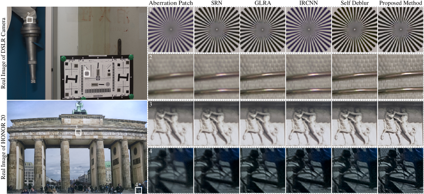
Real-shoot image restoration comparison.
With the testing images taken by the camera (detailed in Sec.6.2), we evaluate the proposed technique with state-of-the-art deblurring methods. As shown in Figure 12, we show two patches of each test image: one patch is near the center of the image, and the other patch is on the edge. We note that the PSFs of the DSLR camera are relatively consistent (as shown in Figure 8), so for the mainstream deblurring algorithms, which are used to deal with globally consistent blur, the restoration of the center and edge of the comparison methods are similar. When compared with other techniques, the results of the proposed approach in the central FOV are similar to those of other methods. In the edge of the image, our result of the DSLR camera is slightly better than those of the other methods. However, for the situation in which the PSFs show a wide range of spatial variation over regions, such as mobile phone cameras, the advantages of our approach are evident. In Figure 12, one can see that the proposed method is superior to all other methods for center and edge restoration. The reconstruction effectively removes the blurring caused by optical aberrations, while the spatial-adaptive network architecture successfully handles the spatially variant PSFs and preserves the texture of the original image. We note that some results of GLRA and IRCNN are somewhat comparable to the proposed method, while in general, our approach can obtain better results in different FOVs. It must be emphasized that the additional input is useful for optical aberration correction because the degradation is highly correlated with the FOV information. Overall, we demonstrate the spatial adaptability of our network architecture. When compared with other methods, the proposed approach is more effective in dealing with the PSFs of spatial variation and therefore is suitable for optical aberration correction.
8. Experimental Assessment
In this section, we take a comprehensive look at the proposed approach and demonstrate its potential applications. First, we assess how much the proposed method improves MTF, chromatismm and line-pair resolution. Second, the restored results are compared with the image postprocessed by HUAWEI ISP, to evaluate the improvement in integrating aberration correction into an ISP system.
8.1. MTF and LPI Enhancement

Aberrations correction vs. HUAWEI ISP.

chro&mtf enhancement.
We compare the chromatism and the MTF of degraded image and recovered image (shown in Figure 14). Though only trained with synthetic data, the proposed method can restore perfect knife edge and greatly improve the MTF results. Moreover, the pixel values of the R, G, and B channels of the reconstructed image are closer to each other, which indicates that our method successfully handles the chromatism between different channels. The lower restored CA curve also proves that the shift between RGB channels is smaller. Moreover, the enhancement of line-pair per inch (LPI) is shown in Figure 12, where the line-pair resolution is improved in the center of the ISO12233 chart. We note that the restored MTF results approach the diffraction limit of the lens, which is the physical limit resolution of an imaging device.
8.2. Aberrations correction vs. HUAWEI ISP
The ultimate goal of the proposed work is to integrate the module of aberration correction into an ISP system and to produce nearly perfect images. In today’s handcrafted ISPs, sharpening is the core method for alleviating the blurring caused by optical aberrations. Unfortunately, the sharpening operation is globally consistent and cannot solve the spatially variant blur. Therefore, it introduces unsolved blur in the boundary of FOV and ”ringing” effect in the center of figure (as shown in Figure 2c). In Figure 13, we compare the results of our proposed pipeline (as shown in Figure 3) and the images generated by HUAWEI ISP (for more results, please refer to the supplementary materials). Obviously, our proposed method adapts to the spatially variant degradation and the results are visually superior to HUAWEI’s ISP. Together with accurate synthetic data and the customized restoration algorithm, we demonstrate that it is possible to handle optical aberrations in postprocessing. This also encourages us to use a lightweight lens for high-quality imaging.
9. Discussion And Conclusion
In this paper, we demonstrated that it is feasible to correct optical aberrations in postprocessing systems. Based on the optical PSF model, the imaging simulation system was developed. Moreover, with synthetic data generated in simulation, we designed the spatial-adaptive network for effective aberration correction.
To be more specific, we constructed an imaging simulation system based on the optical PSF model and the ISP system in the digital camera. Although the lenses in the real world are ever-changing, accurate imaging results can be obtained if crucial parameters are given. In this way, we established the datasets for a specific camera lens. Moreover, to correct the aberrations of optical design, we proposed a spatial-adaptive CNN that combines FOV information to handle aberrations of different sizes and shapes. After that, trained with the simulation datasets, the learned network model was used to map the real degraded images to the restored results. We address spatially variant blurring and chromatism by introducing FOV information, deformable ResBlock, and context block. The proposed method achieves perfect image quality and is more effective in dealing with PSFs varying with space when compared with state-of-the-art deblur methods. Moreover, we successfully corrected the aberrations of the DSLR camera and HUAWEI HONOR 20, which proves that it is a practical method for correcting aberrations and easily transport them to other lenses. Finally, we demonstrate that it is feasible to integrate aberration correction with the existing ISP systems, which will bring great positive benefits.
We find that the introduction of optical information and spatial adaptive capability can result in better recovery, but today’s devices still can’t afford the computational overhead of our postprocessing system. The dedicated NPUs and AI chips equipped on many modern imaging devices still limited to scene classification or postprocessing of a image with low resolution. Today’s optical design and imaging postprocessing system are divisive and we strongly insist that the optical lens and ISP systems can be seen as encoder and decoder, respectively. In this way, the lens-ISP joint design is possible for modern imaging systems. Although this work focuses on the postprocessing system of cameras, we envision that it is practical to jointly design optical lenses and ISP systems for aberration correction or many other tasks such as 3D visual reconstruction.
Acknowledgements.
This work was supported by National Natural Science Foundation of China (NSFC) under Award No.61975175. We also thank Huawei for their support. Finally we would like to thank the TOG reviewers for their valuable comments.References
- (1)
- Abdelhamed et al. (2018) Abdelrahman Abdelhamed, Stephen Lin, and Michael S. Brown. 2018. A High-Quality Denoising Dataset for Smartphone Cameras. In Proceedings of the IEEE Conference on Computer Vision and Pattern Recognition (CVPR). IEEE Computer Society, Salt Lake City, 694–711.
- Agustsson and Timofte (2017) Eirikur Agustsson and Radu Timofte. 2017. NTIRE 2017 Challenge on Single Image Super-Resolution: Dataset and Study. In Proceedings of the IEEE Conference on Computer Vision and Pattern Recognition (CVPR) Workshops. IEEE Computer Society, Hawaii, 126–135.
- Ahi (2017) Kiarash Ahi. 2017. Mathematical modeling of THz point spread function and simulation of THz imaging systems. IEEE Transactions on Terahertz Science and Technology 7, 6 (2017), 747–754. https://doi.org/10.1109/TTHZ.2017.2750690
- Baker and Copson (2003) Bevan B Baker and Edward Thomas Copson. 2003. The mathematical theory of Huygens’ principle. Vol. 329. American Mathematical Soc., Boston.
- Born and Wolf (2013) Max Born and Emil Wolf. 2013. Principles of optics: electromagnetic theory of propagation, interference and diffraction of light. Elsevier, Boston.
- Brooks et al. (2019) Tim Brooks, Ben Mildenhall, Tianfan Xue, Jiawen Chen, Dillon Sharlet, and Jonathan T Barron. 2019. Unprocessing images for learned raw denoising. In Proceedings of the IEEE Conference on Computer Vision and Pattern Recognition. IEEE Computer Soc., Columbus, 11036–11045.
- Buades et al. (2005) Antoni Buades, Bartomeu Coll, and J-M Morel. 2005. A non-local algorithm for image denoising. In 2005 IEEE Computer Society Conference on Computer Vision and Pattern Recognition (CVPR’05), Vol. 2. IEEE, IEEE, Portland, 60–65.
- Cai et al. (2020) J. Cai, H. Zeng, H. Yong, Z. Cao, and L. Zhang. 2020. Toward Real-World Single Image Super-Resolution: A New Benchmark and a New Model. In 2019 IEEE/CVF International Conference on Computer Vision (ICCV). IEEE Computer Soc., Munich, 15–463.
- Chang et al. (2020) Meng Chang, Qi Li, Huajun Feng, and Zhihai Xu. 2020. Spatial-Adaptive Network for Single Image Denoising. arXiv preprint arXiv:2001.10291 26, 10 (2020), 171–187.
- Chen et al. (2018) Chen Chen, Qifeng Chen, Jia Xu, and Vladlen Koltun. 2018. Learning to see in the dark. In Proceedings of the IEEE Conference on Computer Vision and Pattern Recognition. IEEE, Venice, 3291–3300.
- Condat (2010) Laurent Condat. 2010. A simple, fast and efficient approach to denoisaicking: Joint demosaicking and denoising. In 2010 IEEE International Conference on Image Processing. IEEE, IEEE, IEEE, 905–908.
- Dai et al. (2017) Jifeng Dai, Haozhi Qi, Yuwen Xiong, Yi Li, Guodong Zhang, Han Hu, and Yichen Wei. 2017. Deformable convolutional networks. In Proceedings of the IEEE international conference on computer vision. IEEE, IEEE, 764–773.
- Dong et al. (2016) Chao Dong, Chen Change Loy, Kaiming He, and Xiaoou Tang. 2016. Image Super-Resolution Using Deep Convolutional Networks. IEEE Transactions on Pattern Analysis and Machine Intelligence 38, 2 (2016), 295–307. https://doi.org/10.1109/TPAMI.2015.2439281
- Dubois (2006) Eric Dubois. 2006. Filter design for adaptive frequency-domain Bayer demosaicking. In 2006 International Conference on Image Processing. IEEE, IEEE, IEEE, 2705–2708.
- Foi et al. (2008) Alessandro Foi, Mejdi Trimeche, Vladimir Katkovnik, and Karen Egiazarian. 2008. Practical Poissonian-Gaussian Noise Modeling and Fitting for Single-Image Raw-Data. IEEE Transactions on Image Processing 17, 10 (2008), 1737–1754. https://doi.org/10.1109/TIP.2008.2001399
- Gijsenij et al. (2012) Arjan Gijsenij, Theo Gevers, and Joost van de Weijer. 2012. Improving Color Constancy by Photometric Edge Weighting. IEEE Transactions on Pattern Analysis and Machine Intelligence 34, 5 (2012), 918–929. https://doi.org/10.1109/TPAMI.2011.197
- Hasinoff et al. (2016) Samuel W. Hasinoff, Dillon Sharlet, Ryan Geiss, Andrew Adams, Jonathan T. Barron, Florian Kainz, Jiawen Chen, and Marc Levoy. 2016. Burst Photography for High Dynamic Range and Low-Light Imaging on Mobile Cameras. ACM Trans. Graph. 35, 6, Article 192 (nov 2016), 12 pages. https://doi.org/10.1145/2980179.2980254
- Heckbert (1995) Paul Heckbert. 1995. Fourier transforms and the fast Fourier transform (FFT) algorithm. Computer Graphics 2 (1995), 15–463.
- Heide et al. (2013) Felix Heide, Mushfiqur Rouf, Matthias B. Hullin, Bjorn Labitzke, Wolfgang Heidrich, and Andreas Kolb. 2013. High-Quality Computational Imaging through Simple Lenses. ACM Trans. Graph. 32, 5, Article 149 (oct 2013), 14 pages. https://doi.org/10.1145/2516971.2516974
- Heide et al. (2014) Felix Heide, Markus Steinberger, Yun-Ta Tsai, Mushfiqur Rouf, Dawid Paj\kak, Dikpal Reddy, Orazio Gallo, Jing Liu, Wolfgang Heidrich, Karen Egiazarian, Jan Kautz, and Kari Pulli. 2014. FlexISP: A Flexible Camera Image Processing Framework. ACM Trans. Graph. 33, 6, Article 231 (Nov. 2014), 13 pages. https://doi.org/10.1145/2661229.2661260
- Herbel et al. (2018) Jörg Herbel, Tomasz Kacprzak, Adam Amara, Alexandre Refregier, and Aurelien Lucchi. 2018. Fast point spread function modeling with deep learning. Journal of Cosmology and Astroparticle Physics 2018, 07 (jul 2018), 054–054. https://doi.org/10.1088/1475-7516/2018/07/054
- Hirakawa and Parks (2005) K. Hirakawa and T.W. Parks. 2005. Adaptive homogeneity-directed demosaicing algorithm. IEEE Transactions on Image Processing 14, 3 (2005), 360–369. https://doi.org/10.1109/TIP.2004.838691
- Hirsch and Scholkopf (2015) Michael Hirsch and Bernhard Scholkopf. 2015. Self-calibration of optical lenses. In Proceedings of the IEEE International Conference on Computer Vision. IEEE, IEEE, 612–620.
- Ignatov et al. (2017) Andrey Ignatov, Nikolay Kobyshev, Radu Timofte, Kenneth Vanhoey, and Luc Van Gool. 2017. Dslr-quality photos on mobile devices with deep convolutional networks. In Proceedings of the IEEE International Conference on Computer Vision. IEEE, IEEE, 3277–3285.
- Ignatov et al. (2018) Andrey Ignatov, Nikolay Kobyshev, Radu Timofte, Kenneth Vanhoey, and Luc Van Gool. 2018. Wespe: weakly supervised photo enhancer for digital cameras. In Proceedings of the IEEE Conference on Computer Vision and Pattern Recognition Workshops. IEEE, IEEE, 691–700.
- Ignatov and Timofte (2019) Andrey Ignatov and Radu Timofte. 2019. Ntire 2019 challenge on image enhancement: Methods and results. In Proceedings of the IEEE Conference on Computer Vision and Pattern Recognition Workshops. IEEE, IEEE, 0–0.
- Ignatov et al. (2020) Andrey Ignatov, Luc Van Gool, and Radu Timofte. 2020. Replacing mobile camera isp with a single deep learning model. In Proceedings of the IEEE/CVF Conference on Computer Vision and Pattern Recognition Workshops. IEEE, IEEE, 536–537.
- Jemec et al. (2017) Jurij Jemec, Franjo Pernuš, Boštjan Likar, and Miran Bürmen. 2017. 2D sub-pixel point spread function measurement using a virtual point-like source. International journal of computer vision 121, 3 (2017), 391–402.
- Ji et al. (2020) X. Ji, Cao Y, Tai Y, C. Wang, J. Li, and F. Huang. 2020. Real-World Super-Resolution via Kernel Estimation and Noise Injection. In 2020 IEEE/CVF Conference on Computer Vision and Pattern Recognition Workshops (CVPRW). IEEE, IEEE, 15–463.
- Johnson et al. (2016) Justin Johnson, Alexandre Alahi, and Li Fei-Fei. 2016. Perceptual losses for real-time style transfer and super-resolution. In European conference on computer vision. Springer, Springer, Boston, 694–711.
- Kim et al. (2016) Jiwon Kim, Jung Kwon Lee, and Kyoung Mu Lee. 2016. Accurate image super-resolution using very deep convolutional networks. In Proceedings of the IEEE conference on computer vision and pattern recognition. IEEE, Venice, 1646–1654.
- Kwok et al. (2013) N.M. Kwok, H.Y. Shi, Q.P. Ha, G. Fang, S.Y. Chen, and X. Jia. 2013. Simultaneous image color correction and enhancement using particle swarm optimization. Engineering Applications of Artificial Intelligence 26, 10 (2013), 2356–2371. https://doi.org/10.1016/j.engappai.2013.07.023
- Ledig et al. (2017) Christian Ledig, Lucas Theis, Ferenc Huszár, Jose Caballero, Andrew Cunningham, Alejandro Acosta, Andrew Aitken, Alykhan Tejani, Johannes Totz, Zehan Wang, et al. 2017. Photo-realistic single image super-resolution using a generative adversarial network. In Proceedings of the IEEE conference on computer vision and pattern recognition. IEEE, Venice, 4681–4690.
- Li et al. (2008) Xin Li, Bahadir Gunturk, and Lei Zhang. 2008. Image demosaicing: A systematic survey. In Visual Communications and Image Processing 2008, Vol. 6822. International Society for Optics and Photonics, IEEE, Venice, 68221J.
- Lian et al. (2007) Nai-Xiang Lian, Lanlan Chang, Yap-Peng Tan, and Vitali Zagorodnov. 2007. Adaptive Filtering for Color Filter Array Demosaicking. IEEE Transactions on Image Processing 16, 10 (2007), 2515–2525. https://doi.org/10.1109/TIP.2007.904459
- Mahajan (1982) Virendra N Mahajan. 1982. Strehl ratio for primary aberrations: some analytical results for circular and annular pupils. JOSA 72, 9 (1982), 1258–1266.
- Manual (2009) Zemax Manual. 2009. Optical Design Program User’s Guide [R].
- Martin et al. (2001) David Martin, Charless Fowlkes, Doron Tal, and Jitendra Malik. 2001. A database of human segmented natural images and its application to evaluating segmentation algorithms and measuring ecological statistics. In Proceedings Eighth IEEE International Conference on Computer Vision. ICCV 2001, Vol. 2. IEEE, IEEE, Venice, 416–423.
- Mei et al. (2019) Kangfu Mei, Juncheng Li, Jiajie Zhang, Haoyu Wu, Jie Li, and Rui Huang. 2019. Higher-resolution network for image demosaicing and enhancing. In 2019 IEEE/CVF International Conference on Computer Vision Workshop (ICCVW). IEEE, IEEE, Venice, 3441–3448.
- Mosleh et al. (2015) Ali Mosleh, Paul Green, Emmanuel Onzon, Isabelle Begin, and JM Pierre Langlois. 2015. Camera intrinsic blur kernel estimation: A reliable framework. In Proceedings of the IEEE conference on computer vision and pattern recognition. IEEE, Venice, 4961–4968.
- Nah et al. (2017) Seungjun Nah, Tae Hyun Kim, and Kyoung Mu Lee. 2017. Deep multi-scale convolutional neural network for dynamic scene deblurring. In Proceedings of the IEEE Conference on Computer Vision and Pattern Recognition. IEEE, Venice, 3883–3891.
- Pan et al. (2016) Jinshan Pan, Deqing Sun, Hanspeter Pfister, and Ming-Hsuan Yang. 2016. Blind image deblurring using dark channel prior. In Proceedings of the IEEE Conference on Computer Vision and Pattern Recognition. IEEE, Venice, 1628–1636.
- Paul (2014) Gunther Paul. 2014. Huygens’ principle and hyperbolic equations. Academic Press, Venice.
- Paulin-Henriksson et al. (2008) S Paulin-Henriksson, A Amara, L Voigt, A Refregier, and SL Bridle. 2008. Point spread function calibration requirements for dark energy from cosmic shear. Astronomy & Astrophysics 484, 1 (2008), 67–77.
- Peng et al. (2019) Yifan Peng, Qilin Sun, Xiong Dun, Gordon Wetzstein, Wolfgang Heidrich, and Felix Heide. 2019. Learned large field-of-view imaging with thin-plate optics. ACM Trans. Graph. 38, 6 (2019), 219–1.
- Ratnasingam (2019) Sivalogeswaran Ratnasingam. 2019. Deep camera: A fully convolutional neural network for image signal processing. In Proceedings of the IEEE International Conference on Computer Vision Workshops. IEEE, Venice, 0–0.
- Ren et al. (2020) Dongwei Ren, Kai Zhang, Qilong Wang, Qinghua Hu, and Wangmeng Zuo. 2020. Neural blind deconvolution using deep priors. In Proceedings of the IEEE/CVF Conference on Computer Vision and Pattern Recognition. IEEE, Venice, 3341–3350.
- Ren et al. (2018) Wenqi Ren, Jiawei Zhang, Lin Ma, Jinshan Pan, Xiaochun Cao, Wangmeng Zuo, Wei Liu, and Ming-Hsuan Yang. 2018. Deep Non-Blind Deconvolution via Generalized Low-Rank Approximation. In Advances in Neural Information Processing Systems, S. Bengio, H. Wallach, H. Larochelle, K. Grauman, N. Cesa-Bianchi, and R. Garnett (Eds.), Vol. 31. Curran Associates, Inc., 57 Morehouse Ln, Red Hook, NY 12571, USA. https://proceedings.neurips.cc/paper/2018/file/0aa1883c6411f7873cb83dacb17b0afc-Paper.pdf
- Ronneberger et al. (2015) Olaf Ronneberger, Philipp Fischer, and Thomas Brox. 2015. U-net: Convolutional networks for biomedical image segmentation. In International Conference on Medical image computing and computer-assisted intervention. Springer, Springer, Venice, 234–241.
- Sajjadi et al. (2017) Mehdi SM Sajjadi, Bernhard Scholkopf, and Michael Hirsch. 2017. Enhancenet: Single image super-resolution through automated texture synthesis. In Proceedings of the IEEE International Conference on Computer Vision. Springer, Venice, 4491–4500.
- Schroeder (1981) Manfred R Schroeder. 1981. Modulation transfer functions: Definition and measurement. Acta Acustica united with Acustica 49, 3 (1981), 179–182.
- Schuler et al. (2016) Christian J. Schuler, Michael Hirsch, Stefan Harmeling, and Bernhard Schölkopf. 2016. Learning to Deblur. IEEE Transactions on Pattern Analysis and Machine Intelligence 38, 7 (2016), 1439–1451. https://doi.org/10.1109/TPAMI.2015.2481418
- Schwartzburg et al. (2014) Yuliy Schwartzburg, Romain Testuz, Andrea Tagliasacchi, and Mark Pauly. 2014. High-Contrast Computational Caustic Design. ACM Trans. Graph. 33, 4, Article 74 (July 2014), 11 pages. https://doi.org/10.1145/2601097.2601200
- Shi et al. (2016) Wenzhe Shi, Jose Caballero, Ferenc Huszár, Johannes Totz, Andrew P Aitken, Rob Bishop, Daniel Rueckert, and Zehan Wang. 2016. Real-time single image and video super-resolution using an efficient sub-pixel convolutional neural network. In Proceedings of the IEEE conference on computer vision and pattern recognition. Springer, Venice, 1874–1883.
- Shih et al. (2012) Yichang Shih, Brian Guenter, and Neel Joshi. 2012. Image enhancement using calibrated lens simulations. In European Conference on Computer Vision. Springer, Springer, Venice, 42–56.
- Sliusarev (1984) Georgii Georgievich Sliusarev. 1984. Aberration and optical design theory. ahl 17, 10 (1984), 1737–1754.
- Smith (2005) Warren J Smith. 2005. Modern lens design. American Mathematical Soc., Boston.
- Smith (2008) Warren J Smith. 2008. Modern optical engineering. Tata McGraw-Hill Education, Boston.
- Sun et al. (2015) Jian Sun, Wenfei Cao, Zongben Xu, and Jean Ponce. 2015. Learning a convolutional neural network for non-uniform motion blur removal. In Proceedings of the IEEE Conference on Computer Vision and Pattern Recognition. IEEE, Venice, 769–777.
- Sun et al. (2017) Tiancheng Sun, Yifan Peng, and Wolfgang Heidrich. 2017. Revisiting cross-channel information transfer for chromatic aberration correction. In Proceedings of the IEEE International Conference on Computer Vision. IEEE, Venice, 3248–3256.
- Tao et al. (2018) Xin Tao, Hongyun Gao, Xiaoyong Shen, Jue Wang, and Jiaya Jia. 2018. Scale-recurrent network for deep image deblurring. In Proceedings of the IEEE Conference on Computer Vision and Pattern Recognition. IEEE, Venice, 8174–8182.
- van de Weijer et al. (2007) Joost van de Weijer, Theo Gevers, and Arjan Gijsenij. 2007. Edge-Based Color Constancy. IEEE Transactions on Image Processing 16, 9 (2007), 2207–2214. https://doi.org/10.1109/TIP.2007.901808
- Vedaldi and Fulkerson (2010) Andrea Vedaldi and Brian Fulkerson. 2010. VLFeat: An open and portable library of computer vision algorithms. In Proceedings of the 18th ACM international conference on Multimedia. IEEE, Venice, 1469–1472.
- Wang et al. (2019) Xintao Wang, Kelvin CK Chan, Ke Yu, Chao Dong, and Chen Change Loy. 2019. Edvr: Video restoration with enhanced deformable convolutional networks. In Proceedings of the IEEE Conference on Computer Vision and Pattern Recognition Workshops. IEEE, Venice, 0–0.
- Wang et al. (2018) Xintao Wang, Ke Yu, Shixiang Wu, Jinjin Gu, Yihao Liu, Chao Dong, Yu Qiao, and Chen Change Loy. 2018. Esrgan: Enhanced super-resolution generative adversarial networks. In Proceedings of the European Conference on Computer Vision (ECCV) Workshops. IEEE, Venice, 0–0.
- Westphal et al. (2002) Volker Westphal, Andrew M Rollins, Sunita Radhakrishnan, and Joseph A Izatt. 2002. Correction of geometric and refractive image distortions in optical coherence tomography applying Fermat’s principle. Optics Express 10, 9 (2002), 397–404.
- Yan et al. (2019) Qingsen Yan, Dong Gong, Qinfeng Shi, Anton van den Hengel, Chunhua Shen, Ian Reid, and Yanning Zhang. 2019. Attention-guided network for ghost-free high dynamic range imaging. In Proceedings of the IEEE Conference on Computer Vision and Pattern Recognition. IEEE, Venice, 1751–1760.
- Zhang et al. (2017) Kai Zhang, Wangmeng Zuo, Shuhang Gu, and Lei Zhang. 2017. Learning Deep CNN Denoiser Prior for Image Restoration. In IEEE Conference on Computer Vision and Pattern Recognition. IEEE, Venice, 3929–3938.
- Zhang et al. (2019) Xuaner Zhang, Qifeng Chen, Ren Ng, and Vladlen Koltun. 2019. Zoom to learn, learn to zoom. In Proceedings of the IEEE Conference on Computer Vision and Pattern Recognition. IEEE, Venice, 3762–3770.
- Zhenggang (2016) LI Zhenggang. 2016. Periscope lens and terminal device. US Patent 9,523,847.
- Zhu et al. (2019) Xizhou Zhu, Han Hu, Stephen Lin, and Jifeng Dai. 2019. Deformable convnets v2: More deformable, better results. In Proceedings of the IEEE Conference on Computer Vision and Pattern Recognition. IEEE, Venice, 9308–9316.