OpenMixup: Open Mixup Toolbox and Benchmark for Visual Representation Learning

Siyuan Li^1,2   Zedong Wang^1∗  Zicheng Liu^1,2  Juanxi Tian¹  Di Wu^1,2
Cheng Tan^1,2  Weiyang Jin¹  Stan Z. Li^1†
¹AI Lab, Research Center for Industries of the Future, Westlake University, Hangzhou, China
²Zhejiang University, Hangzhou, China
Equal contribution.    ^†Corrsponding author.

Abstract

Mixup augmentation has emerged as a widely used technique for improving the generalization ability of deep neural networks (DNNs). However, the lack of standardized implementations and benchmarks has impeded recent progress, resulting in poor reproducibility, unfair comparisons, and conflicting insights. In this paper, we introduce OpenMixup, the first mixup augmentation codebase and benchmark for visual representation learning. Specifically, we train 18 representative mixup baselines from scratch and rigorously evaluate them across 11 image datasets of varying scales and granularity, ranging from fine-grained scenarios to complex non-iconic scenes. We also open-source our modular codebase including a collection of popular vision backbones, optimization strategies, and analysis toolkits, which not only supports the benchmarking but enables broader mixup applications beyond classification, such as self-supervised learning and regression tasks. Through experiments and empirical analysis, we gain observations and insights on mixup performance-efficiency trade-offs, generalization, and optimization behaviors, and thereby identify preferred choices for different needs. To the best of our knowledge, OpenMixup has facilitated several recent studies. We believe this work can further advance reproducible mixup augmentation research and thereby lay a solid ground for future progress in the community. The source code will be publicly available.

Refer to caption — Figure 1: Radar plot of top-1 accuracy for representative mixup baselines on 11 classification datasets.

1 Introduction

Data mixing, or mixup, has proven effective in enhancing the generalization ability of DNNs, with notable success in visual classification tasks. The pioneering Mixup (Zhang et al., 2018) proposes to generate mixed training examples through the convex combination of two input samples and their corresponding one-hot labels. By encouraging models to learn smoother decision boundaries, mixup effectively reduces overfitting and thus improves the overall performance. ManifoldMix (Verma et al., 2019) and PatchUp (Faramarzi et al., 2020) extend this operation to the hidden space. CutMix (Yun et al., 2019) presents an alternative approach, where an input rectangular region is randomly cut and pasted onto the target in the identical location. Subsequent works (Harris et al., 2020; ha Lee et al., 2020; Baek et al., 2021) have focused on designing more complex hand-crafted policies to generate diverse and informative mixed samples, which can all be categorized as static mixing methods.

Despite efforts to incorporate saliency information into static mixing framework (Walawalkar et al., 2020; Uddin et al., 2020; Qin et al., 2023), they still struggle to ensure the inclusion of desired targets in the mixed samples, which may result in the issue of label mismatches. To address this problem, a new class of optimization-based methods, termed dynamic mixing, has been proposed, as illustrated in the second row of Figure 2. PuzzleMix (Kim et al., 2020) and Co-Mixup (Kim et al., 2021) are two notable studies that leverage optimal transport to improve offline mask determination. More recently, TransMix (Chen et al., 2022), TokenMix (Liu et al., 2022a), MixPro (Zhao et al., 2023), and SMMix (Chen et al., 2023) are specifically tailored for Vision Transformers (Dosovitskiy et al., 2021). The AutoMix series (Liu et al., 2022d; Qin et al., 2024) introduces a brand-new mixup learning paradigm, where mixed samples are computed by an online-optimizable generator in an end-to-end manner. These emerging dynamic approaches represent a promising avenue for generating semantically richer training samples that align with the underlying structure of input data.

Why do we call for a mixup augmentation benchmark? While dynamic methods have shown signs of surpassing the static ones, their indirect optimization process incurs significant computational overhead, which limits their efficiency and applicability. Therefore, without a systematic understanding, it is uncertain if dynamic mixup serves as the superior alternative in vision tasks. Moreover, a thorough and standardized evaluation of different dynamic methods is also missing in the community. Benchmark is exactly the way to establish such an understanding, which plays a pivotal role in driving research progress by integrating an agreed-upon set of tasks, impartial comparisons, and assessment criteria. To the best of our knowledge, however, there have been no such comprehensive benchmarks for mixup augmentation to facilitate unbiased comparisons and practical use in visual recognition.

Why do we need an open-source mixup codebase? Notably, most existing mixup techniques are crafted with diverse settings, tricks, and implementations, each with its own coding style. This lack of standardization not only hinders user-friendly reproduction and deployment but impedes further development, thus imposing costly trial-and-error on practitioners to determine the most appropriate mixup strategy for their specific needs in real-world applications. Hence, it is essential to develop a unified mixup visual representation learning codebase for standardized data pre-processing, mixup development, network architecture selection, model training, evaluation, and empirical analysis.

In this paper, we present OpenMixup, the first comprehensive benchmark for mixup augmentation in vision tasks. Unlike previous work (Naveed, 2021; Lewy & Mańdziuk, 2023), we train and evaluate 18 methods that represent the foremost strands on 11 diverse image datasets, as illustrated in Figure 1. We also open-source a standardized mixup codebase for visual representation learning, where the overall framework is built up with modular components for data pre-processing, mixup augmentation, network backbone selection, optimization, and evaluations. The codebase not only powers our benchmarking but supports broader relatively under-explored mixup applications beyond classification, such as semi-supervised learning (Berthelot et al., 2019), self-supervised learning (Kalantidis et al., 2020; Shen et al., 2022), and dense prediction tasks (He et al., 2017; Bochkovskiy et al., 2020).

Furthermore, insightful observations are obtained by incorporating multiple evaluation metrics and analysis toolkits in our codebase, including GPU memory usage (Figure 4), loss landscape (Figure 5(c)), Power Law (PL) exponent alpha metrics (Figure 6), robustness and calibration (Table A8), etc. For instance, despite the key role static mixing plays in today’s deep learning systems, we surprisingly find that its generalizability over diverse datasets and backbones is significantly inferior to that of dynamic algorithms. By ranking the performance and efficiency trade-offs, we reveal that recent dynamic methods have already outperformed the static ones. This may suggest a promising breakthrough for mixup augmentation, provided that the dynamic computational overhead can be further reduced. Overall, we believe these insights can facilitate better evaluation and comparisons of mixup methods, enabling a systematic understanding and thus paving the way for further advancements.

Since such a first-of-its benchmark can be rather time- and resource-consuming and most current advances have focused on and stemmed from visual classification tasks, we centralize our benchmarking scope on classification while extending it to broader mixup applications with transfer learning. Meanwhile, we have already supported these downstream tasks and datasets in our open-source codebase, allowing practitioners to customize their mixup algorithms, models, and training setups in these relatively under-explored scenarios. Our key contributions can be summarized as follows:

•

We introduce OpenMixup, the first comprehensive benchmarking study for mixup augmentation, where 18 representative baselines are trained from scratch and rigorously evaluated on 11 visual classification datasets, ranging from non-iconic scenes to gray-scale, fine-grained, and long tail scenarios. By providing a standard testbed and a rich set of evaluation protocols, OpenMixup enables fair comparisons, thorough assessment, and analysis of different mixup strategies.
•

To support reproducible mixup research and user-friendly method deployment, we provide an open-source codebase for visual representation learning. The codebase incorporates standardized modules for data pre-processing, mixup augmentation, backbone selection, optimization policies, and distributed training functionalities. Beyond the benchmark itself, our OpenMixup codebase is readily extensible and has supported semi- and self-supervised learning and visual attribute regression tasks, which further enhances its utility and potential benefits to the community.
•

Observations and insights are obtained through extensive analysis. We investigate the generalization ability of all evaluated mixup baselines across diverse datasets and backbones, compare their GPU memory footprint and computational cost, visualize the loss landscape and PL exponent alpha metrics to understand optimization behavior, and evaluate robustness against input corruptions and calibration performance. Furthermore, we establish comprehensive rankings in terms of their performance and applicability (efficiency and versatility), offering clear method guidelines for specific requirements. These findings not only present a firm grasp of the current mixup augmentation landscape but shed light on promising avenues for future advancements.

2 Background and Related Work

2.1 Problem Definition

Mixup Training.

We first consider the general image classification tasks with $k$ different classes: given a finite set of $n$ image samples $X=[x_{i}]_{i=1}^{n}\in\mathbb{R}^{n\times W\times H\times C}$ and their corresponding ground-truth class labels $Y=[y_{i}]_{i=1}^{n}\in\mathbb{R}^{n\times k}$ , encoded by a one-hot vector $y_{i}\in\mathbb{R}^{k}$ . We attempt to seek the mapping from input data $x_{i}$ to its class label $y_{i}$ modeled through a deep neural network $f_{\theta}:x\longmapsto y$ with parameters $\theta$ by optimizing a classification loss $\ell(.)$ , say the cross entropy (CE) loss,

\ell_{CE}(f_{\theta}(x),y)=-y\log f_{\theta}(x).\vspace{-0.25em}

(1)

Then we consider the mixup classification task: given a sample mixing function $h$ , a label mixing function $g$ , and a mixing ratio $\lambda$ sampled from $Beta(\alpha,\alpha)$ distribution, we can generate the mixed data $X_{mix}$ with $x_{mix}=h(x_{i},x_{j},\lambda)$ and the mixed label $Y_{mix}$ with $y_{mix}=g(y_{i},y_{j},\lambda)$ , where $\alpha$ is a hyper-parameter. Similarly, we learn $f_{\theta}:x_{mix}\longmapsto y_{mix}$ by the mixup cross-entropy (MCE) loss,

\ell_{MCE}=\lambda\ell_{CE}(f_{\theta}(x_{mix}),y_{i})+(1-\lambda)\ell_{CE}(f_{\theta}(x_{mix}),y_{j}).\vspace{-0.5em}

(2)

Mixup Reformulation.

Comparing Eq. (1) and Eq. (2), the mixup training has the following features: (1) extra mixup policies, $g$ and $h$ , are required to generate $X_{mix}$ and $Y_{mix}$ . (2) the classification performance of $f_{\theta}$ depends on the generation policy of mixup. Naturally, we can split the mixup task into two complementary sub-tasks: (i) mixed sample generation and (ii) mixup classification (learning objective). Notice that the sub-task (i) is subordinate to (ii) because the final goal is to obtain a stronger classifier. Therefore, from this perspective, we regard the mixup generation as an auxiliary task for the classification task. Since $g$ is generally designed as a linear interpolation, i.e., $g(y_{i},y_{j},\lambda)=\lambda y_{i}+(1-\lambda)y_{j}$ , $h$ becomes the key function to determine the performance of the model. Generalizing previous offline methods, we define a parametric mixup policy $h_{\phi}$ as the sub-task with another set of parameters $\phi$ . The final goal is to optimize $\ell_{MCE}$ given $\theta$ and $\phi$ as:

\mathop{{\rm min}}\limits_{\theta,~{}\phi}\ell_{MCE}\Big{(}f_{\theta}\big{(}h_{\phi}(x_{i},x_{j},\lambda)\big{)},g(y_{i},y_{j},\lambda)\Big{)}.\vspace{-0.5em}

(3)

2.2 Sample Mixing

Within the realm of visual classification, prior research has primarily concentrated on refining the sample mixing strategies rather than the label mixing ones. In this context, most sample mixing methods are categorized into two groups: static policies and dynamic policies, as presented in Table 1.

Static Policies.

The sample mixing procedure in all static policies is conducted in a hand-crafted manner. Mixup (Zhang et al., 2018) first generates artificially mixed data through the convex combination of two selected input samples and their associated one-hot labels. ManifoldMix variants (Verma et al., 2019; Faramarzi et al., 2020) extend the same technique to latent space for smoother feature mixing. Subsequently, CutMix (Yun et al., 2019) involves the random replacement of a certain rectangular region inside the input sample while concurrently employing Drop Patch throughout the mixing process. Inspired by CutMix, several researchers in the community have explored the use of saliency information (Uddin et al., 2020) to pilot mixing patches, while others have developed more complex hand-crafted sample mixing strategies (Harris et al., 2020; Baek et al., 2021).

Table 1: Overview of all supported vision Mixup augmentation methods in OpenMixup. Note that Mixup and CutMix in label mixing indicate mixing the labels of two samples by linear interpolation or computing cut squares. The Perf., App., and Overall denote the performance, applicability, and overall rankings of all methods, which are derived from average rankings across baselines (view B.5).

Method	Category	Publication	Sample Mixing	Label Mixing	Extra Cost	ViT only	Perf.	App.	Overall
Mixup (Zhang et al., 2018)	Static	ICLR’2018	Hand-crafted Interpolation	Mixup	✗	✗	15	1	10
CutMix (Yun et al., 2019)	Static	ICCV’2019	Hand-crafted Cutting	CutMix	✗	✗	13	1	8
DeiT (CutMix+Mixup) (Touvron et al., 2021)	Static	ICML’2021	CutMix+Mixup	CutMix+Mixup	✗	✗	7	1	3
SmoothMix (ha Lee et al., 2020)	Static	CVPRW’2020	Hand-crafted Cutting	CutMix	✗	✗	18	1	13
GridMix (Baek et al., 2021)	Static	PR’2021	Hand-crafted Cutting	CutMix	✗	✗	17	1	12
ResizeMix (Qin et al., 2023)	Static	CVMJ’2023	Hand-crafted Cutting	CutMix	✗	✗	10	1	5
ManifoldMix (Verma et al., 2019)	Static	ICML’2019	Latent-space Mixup	Mixup	✗	✗	14	1	9
FMix (Harris et al., 2020)	Static	arXiv’2020	Fourier-guided Cutting	CutMix	✗	✗	16	1	11
AttentiveMix (Walawalkar et al., 2020)	Static	ICASSP’2020	Pretraining-guided Cutting	CutMix	✓	✗	9	3	6
SaliencyMix (Uddin et al., 2020)	Static	ICLR’2021	Saliency-guided Cutting	CutMix	✗	✗	11	1	6
PuzzleMix (Kim et al., 2020)	Dynamic	ICML’2020	Optimal-transported Cutting	CutMix	✓	✗	8	4	6
AlignMix (Venkataramanan et al., 2022)	Dynamic	CVPR’2022	Optimal-transported Interpolation	CutMix	✓	✗	12	2	8
AutoMix (Liu et al., 2022d)	Dynamic	ECCV’2022	End-to-end-learned Cutting	CutMix	✓	✗	3	6	4
SAMix (Li et al., 2021)	Dynamic	arXiv’2021	End-to-end-learned Cutting	CutMix	✓	✗	1	5	1
AdAutoMix (Qin et al., 2024)	Dynamic	ICLR’2024	End-to-end-learned Cutting	CutMix	✓	✗	2	7	4
TransMix (Chen et al., 2022)	Dynamic	CVPR’2022	CutMix+Mixup	Attention-guided	✗	✓	5	8	7
SMMix (Chen et al., 2023)	Dynamic	ICCV’2023	CutMix+Mixup	Attention-guided	✗	✓	4	8	6
DecoupledMix (Liu et al., 2022c)	Static	NeurIPS’2023	Any Sample Mixing Policies	DecoupledMix	✗	✗	6	1	2

Dynamic Policies.

In contrast to static mixing, dynamic strategies are proposed to incorporate sample mixing into an adaptive optimization-based framework. PuzzleMix variants (Kim et al., 2020; 2021) introduce combinatorial optimization-based mixing policies in accordance with saliency maximization. SuperMix variants (Dabouei et al., 2021; Walawalkar et al., 2020) utilize pre-trained teacher models to compute smooth and optimized samples. Distinctively, AutoMix variants (Liu et al., 2022d; Li et al., 2021) reformulate the overall framework of sample mixing into an online-optimizable fashion where the model learns to generate the mixed samples in an end-to-end manner.

2.3 Label Mixing

Mixup (Zhang et al., 2018) and CutMix (Yun et al., 2019) are two widely-recognized label mixing techniques, both of which are static. Recently, there has been a notable emphasis among researchers on advancing label mixing approaches, which attain more favorable performance upon certain sample mixing policies. Based on Transformers, TransMix variants (Chen et al., 2022; Liu et al., 2022a; Choi et al., 2022; Chen et al., 2023) are proposed to utilize class tokens and attention maps to adjust the mixing ratio. A decoupled mixup objective (Liu et al., 2022c) is introduced to force models to focus on those hard mixed samples, which can be plugged into different sample mixing policies. Holistically, most existing studies strive for advanced sample mixing designs rather than label mixing.

2.4 Other Applications

Recently, mixup augmentation also has shown promise in more vision applications, such as semi-supervised learning (Berthelot et al., 2019; Liu et al., 2022c), self-supervised pre-training (Kalantidis et al., 2020; Shen et al., 2022), and visual attribute regression (Wu et al., 2022; Bochkovskiy et al., 2020). Although these fields are not as extensively studied as classification, our OpenMixup codebase has been designed to support them by including the necessary task settings and datasets. Its modular and extensible architecture allows researchers and practitioners in the community to effortlessly adapt and extend their models to accommodate the specific requirements of these tasks, enabling them to quickly set up experiments without building the entire pipeline from scratch. Moreover, our codebase will be well-positioned to accelerate the development of future benchmarks, ultimately contributing to the advancement of mixup augmentation across a diversity of visual representation learning tasks.

3 OpenMixup

This section introduces our OpenMixup codebase framework and benchmark from four key aspects: supported methods and tasks, evaluation metrics, and experimental pipeline. OpenMixup provides a unified framework implemented in PyTorch (Paszke et al., 2019) for mixup model design, training, and evaluation. The framework references MMClassification (Contributors, 2020a) and follows the OpenMMLab coding style. We start with an overview of its composition. As shown in Figure 3, the whole training process here is fragmented into multiple components, including model architecture (.openmixup.models), data pre-processing (.openmixup.datasets), mixup policies (.openmixup.models.utils.augments), script tools (.tools) etc. For instance, vision models are summarized into modular building blocks (e.g., backbone, neck, head etc.) in .openmixup.models. This modular architecture enables practitioners to easily craft models by incorporating different components through configuration files in .configs. As such, users can readily customize their specified vision models and training strategies. In addition, benchmarking configuration (.benchmarks) and results (.tools.model zoos) are also provided in the codebase. Additional benchmarking configurations and details are discussed below.

3.1 Benchmarked Methods

OpenMixup has implemented 17 representative mixup augmentation algorithms and 19 convolutional neural network and Transformer model architectures (gathered in .openmixup.models) across 12 diverse image datasets for supervised visual classification. We summarize these mixup methods in Table 1, along with their corresponding conference/journal, the types of employed sample, and label mixing policies, properties, and rankings. For sample mixing, Mixup (Zhang et al., 2018) and ManifoldMix (Verma et al., 2019) perform hand-crafted convex interpolation. CutMix (Yun et al., 2019), SmoothMix (ha Lee et al., 2020), GridMix (Baek et al., 2021) and ResizeMix (Qin et al., 2023) implement hand-crafted cutting policy. FMix (Harris et al., 2020) utilizes Fourier-guided cutting. AttentiveMix (Walawalkar et al., 2020) and SaliencyMix (Uddin et al., 2020) apply pretraining-guided and saliency-guided cutting, respectively. Some dynamic approaches like PuzzleMix (Kim et al., 2020) and AlignMix (Venkataramanan et al., 2022) utilize optimal transport-based cutting and interpolation. AutoMix (Liu et al., 2022d) and SAMix (Li et al., 2021) perform end-to-end online-optimizable cutting-based approaches. As for the label mixing, most methods apply Mixup (Zhang et al., 2018) or CutMix (Yun et al., 2019), while the latest mixup methods for visual transformers (TransMix (Chen et al., 2022), TokenMix (Liu et al., 2022a), and SMMix (Chen et al., 2023)), as well as DecoupledMix (Liu et al., 2022c) exploit attention maps and a decoupled framework respectfully instead, which incorporate CutMix variants as its sample mixing strategy. Such a wide scope of supported methods enables a comprehensive benchmarking analysis on visual classification.

3.2 Benchmarking Tasks

We provide detailed descriptions of the 12 open-source datasets as shown in Table 2. These datasets can be classified into four categories below: (1) Small-scale classification: We conduct benchmarking studies on small-scale datasets to provide an accessible benchmarking reference. CIFAR-10/100 (Krizhevsky et al., 2009) consists of 60,000 color images in 32 $\times$ 32 resolutions. Tiny-ImageNet (Tiny) (Chrabaszcz et al., 2017) and STL-10 (Coates et al., 2011) are two re-scale versions of ImageNet-1K in the size of 64 $\times$ 64 and 96 $\times$ 96. FashionMNIST (Xiao et al., 2017) is the advanced version of MNIST, which contains gray-scale images of clothing. (2) Large-scale classification: The large-scale dataset is employed to evaluate mixup algorithms against the most standardized procedure, which can also support the prevailing ViT architecture. ImageNet-1K (IN-1K) (Russakovsky et al., 2015) is a well-known challenging dataset for image classification with 1000 classes. (3) Fine-grained classification: To investigate the effectiveness of mixup methods in complex inter-class relationships and long-tail scenarios, we conduct a comprehensive evaluation of fine-grained classification datasets, which can also be classified into small-scale and large-scale scenarios. (i) Small-scale scenarios: The datasets for small-scale fine-grained evaluation scenario are CUB-200-2011 (CUB) (Wah et al., 2011) and FGVC-Aircraft (Aircraft) (Maji et al., 2013), which contains a total of 200 wild bird species and 100 classes of airplanes. (ii) Large-scale scenarios: The datasets for large-scale fine-grained evaluation scenarios are iNaturalist2017 (iNat2017) (Horn et al., 2018) and iNaturalist2018 (iNat2018) (Horn et al., 2018), which contain 5,089 and 8,142 natural categories. Both the iNat2017 and iNat2018 own 7 major categories and are also long-tail datasets with scenic images (i.e., the fore-ground target is within large backgrounds). (4) Scenic classification: Scenic classification evaluations are also conducted to investigate the performance of different mixup augmentation methods in complex non-iconic scenarios on Places205 (Zhou et al., 2014).

3.3 Evaluation Metrics and Tools

We comprehensively evaluate the beneficial properties of mixup augmentation algorithms on the aforementioned vision tasks through the use of various metrics and visualization analysis tools in a rigorous manner. Overall, the evaluation methodologies can be classified into two distinct divisions, namely performance metric and empirical analysis. For the performance metrics, classification accuracy and robustness against corruption are two performance indicators examined. As for empirical analysis, experiments on calibrations, CAM visualization, loss landscape, the plotting of training loss, and validation accuracy curves are conducted. The utilization of these approaches is contingent upon their distinct properties, enabling user-friendly deployment for designated purposes and demands.

Table 2: The detailed information of supported visual classification datasets in OpenMixup.

Datasets	Category	Source	Classes	Resolution	Train images	Test images
CIFAR-10 (Krizhevsky et al., 2009)	Iconic	link	10	32 $\times$ 32	50,000	10,000
CIFAR-100 (Krizhevsky et al., 2009)	Iconic	link	100	32 $\times$ 32	50,000	10,000
FashionMNIST (Xiao et al., 2017)	Gray-scale	link	10	28 $\times$ 28	50,000	10,000
STL-10 (Coates et al., 2011)	Iconic	link	10	96 $\times$ 96	50,00	8,000
Tiny-ImageNet (Chrabaszcz et al., 2017)	Iconic	link	200	64 $\times$ 64	10,000	10,000
ImageNet-1K (Russakovsky et al., 2015)	Iconic	link	1000	469 $\times$ 387	1,281,167	50,000
CUB-200-2011 (Wah et al., 2011)	Fine-grained	link	200	224 $\times$ 224	5,994	5,794
FGVC-Aircraft (Maji et al., 2013)	Fine-grained	link	100	224 $\times$ 224	6,667	3,333
iNaturalist2017 Horn et al. (2018)	Fine-grained & longtail	link	5089	224 $\times$ 224	579,184	95,986
iNaturalist2018 Horn et al. (2018)	Fine-grained & longtail	link	8142	224 $\times$ 224	437,512	24,426
Places205 (Zhou et al., 2014)	Scenic	link	205	224 $\times$ 224	2,448,873	41,000

Performance Metric.

(1) Accuracy and training costs: We adopt top-1 accuracy, total training hours, and GPU memory to evaluate all mixup methods’ classification performance and training costs. (2) Robustness: We evaluate the robustness against corruptions of the methods on CIFAR-100-C and ImageNet-C (Russakovsky et al., 2015), which is designed for evaluating the corruption robustness and provides 19 different corruptions, e.g., noise and blur etc. (3) Transferability to downstream tasks: We evaluate the transferability of existing methods to object detection based on Faster R-CNN (Ren et al., 2015) and Mask R-CNN (He et al., 2017) on COCO train2017 (Lin et al., 2014), initializing with trained models on ImageNet. We also transfer these methods to semantic segmentation on ADE20K (Zhou et al., 2018). Please refer to Appendix B.4 for details.

Empirical Analysis.

(1) Calibrations: To verify the calibration of existing methods, we evaluate them by the expected calibration error (ECE) on CIFAR-100 (Krizhevsky et al., 2009), i.e., the absolute discrepancy between accuracy and confidence. (2) CAM visualization: We utilize mixed sample visualization, a series of CAM variants (Chattopadhyay et al., 2018; Muhammad & Yeasin, 2020) (e.g., Grad-CAM (Selvaraju et al., 2019)) to directly analyze the classification accuracy and especially the localization capabilities of mixup augmentation algorithms through top-1 top-2 accuracy predicted targets. (3) Loss landscape: We apply loss landscape evaluation (Li et al., 2018) to further analyze the degree of loss smoothness of different mixup augmentation methods. (4) Training loss and accuracy curve: We plot the training losses and validation accuracy curves of various mixup methods to analyze the training stability, the ability to prevent over-fitting, and convergence speed. (5) Quality metric of learned weights: Employing WeightWatch (Martin et al., 2021), we plot the Power Law (PL) exponent alpha metric of learned parameters with mixup algorithms to study their properties on different scenarios, e.g., acting as the regularizer to prevent overfitting or expanding more data as the augmentation technique to learn better representations.

3.4 Experimental Pipeline of OpenMixup Codebase

OpenMixup provides a unified training pipeline that offers a consistent workflow across various computer vision tasks, as illustrated in Figure A1. Taking image classification as an example, we can outline the overall training process as follows. (i) Data preparation: Users first select the appropriate dataset and pre-processing techniques from our supported data pipeline. (ii) Model architecture: The openmixup.models module serves as a component library for building desired model architectures. (iii) Configuration: Users can easily customize their experimental settings using Python configuration files under .configs.classification. These files allow for the specification of datasets, mixup strategies, neural networks, and schedulers. (iv) Execution: The .tools directory not only provides hardware support for distributed training but offers utility functionalities, such as feature visualization, model analysis, and result summarization, which can further facilitate empirical analysis. We also provide comprehensive online user documents, including detailed guidelines for installation and getting started instructions, all the benchmarking results, and awesome lists of related works in mixup augmentation, etc., which ensures that both researchers and practitioners in the community can effectively leverage our OpenMixup for their specific needs.

4 Experiment and Analysis

4.1 Implementation Details

We conduct essential benchmarking experiments of image classification on various scenarios with diverse evaluation metrics. For a fair comparison, grid search is performed for the shared hyper-parameter $\alpha\in\{0.1,0.2,0.5,1,2,4\}$ of supported mixup variants while the rest of the hyper-parameters follow the original papers. Vanilla denotes the classification baseline without any mixup augmentations. All experiments are conducted on Ubuntu workstations with Tesla V100 or NVIDIA A100 GPUs and report the mean results of three trials. Appendix B provides full visual classification results, Appendix B.4 presents our transfer learning results for object detection and semantic segmentation, and Appendix C conduct verification of the reproduction guarantee in OpenMixup.

Table 3: Top-1 accuracy (%) on CIFAR-10/100 and Tiny-ImageNet (Tiny) based on ResNet (R), Wide-ResNet (WRN), and ResNeXt (RX) backbones.

Datasets	CIFAR-10	CIFAR-100	Tiny
Backbones	R-18	WRN-28-8	RX-50
Epochs	800 ep	800 ep	400 ep
Vanilla	95.50	81.63	65.04
Mixup	96.62	82.82	66.36
CutMix	96.68	84.45	66.47
ManifoldMix	96.71	83.24	67.30
SmoothMix	96.17	82.09	68.61
AttentiveMix	96.63	84.34	67.42
SaliencyMix	96.20	84.35	66.55
FMix	96.18	84.21	65.08
GridMix	96.56	84.24	69.12
ResizeMix	96.76	84.87	65.87
PuzzleMix	97.10	85.02	67.83
Co-Mixup	97.15	85.05	68.02
AlignMix	97.05	84.87	68.74
AutoMix	97.34	85.18	70.72
SAMix	97.50	85.50	72.18
AdAutoMix	97.55	85.32	72.89
Decoupled	96.95	84.88	67.46

Table 4: Top-1 accuracy (%) on ImageNet-1K using PyTorch-style, RSB A2/A3, and DeiT settings based on CNN and Transformer architectures, including ResNet (R), MobileNet.V2 (Mob.V2), DeiT-S, and Swin-T.

Backbones	R-50	R-50	Mob.V2 1x	DeiT-S	Swin-T
Epochs	100 ep	100 ep	300 ep	300 ep	300 ep
Settings	PyTorch	RSB A3	RSB A2	DeiT	DeiT
Vanilla	76.83	77.27	71.05	75.66	80.21
Mixup	77.12	77.66	72.78	77.72	81.01
CutMix	77.17	77.62	72.23	80.13	81.23
DeiT / RSB	77.35	78.08	72.87	79.80	81.20
ManifoldMix	77.01	77.78	72.34	78.03	81.15
AttentiveMix	77.28	77.46	70.30	80.32	81.29
SaliencyMix	77.14	77.93	72.07	79.88	81.37
FMix	77.19	77.76	72.79	80.45	81.47
ResizeMix	77.42	77.85	72.50	78.61	81.36
PuzzleMix	77.54	78.02	72.85	77.37	79.60
AutoMix	77.91	78.44	73.19	80.78	81.80
SAMix	78.06	78.64	73.42	80.94	81.87
AdAutoMix	78.04	78.54	-	80.81	81.75
TransMix	-	-	-	80.68	81.80
SMMix	-	-	-	81.10	81.80

Small-scale Benchmarks.

We first provide standard mixup image classification benchmarks on five small datasets with two settings. (a) The classical settings with the CIFAR version of ResNet variants (He et al., 2016; Xie et al., 2017), i.e., replacing the $7\times 7$ convolution and MaxPooling by a $3\times 3$ convolution. We use $32\times 32$ , $64\times 64$ , and $28\times 28$ input resolutions for CIFAR-10/100, Tiny-ImageNet, and FashionMNIST, while using the normal ResNet for STL-10. We train vision models for multiple epochs from the stretch with SGD optimizer and a batch size of 100, as shown in Table 3 and Appendix B.2. (b) The modern training settings following DeiT (Touvron et al., 2021) on CIFAR-100, using $224\times 224$ and $32\times 32$ resolutions for Transformers (DeiT-S (Touvron et al., 2021) and Swin-T (Liu et al., 2021)) and ConvNeXt-T (Liu et al., 2022b) as shown in Table A7.

Standard ImageNet-1K Benchmarks.

For visual augmentation and network architecture communities, ImageNet-1K is a well-known standard dataset. We support three popular training recipes: (a) PyTorch-style (He et al., 2016) setting for classifical CNNs; (b) timm RSB A2/A3 (Wightman et al., 2021) settings; (c) DeiT (Touvron et al., 2021) setting for ViT-based models. Evaluation is performed on 224 $\times$ 224 resolutions with CenterCrop. Popular network architectures are considered: ResNet (He et al., 2016), Wide-ResNet (Zagoruyko & Komodakis, 2016), ResNeXt (Xie et al., 2017), MobileNet.V2 (Sandler et al., 2018), EfficientNet (Tan & Le, 2019), DeiT (Touvron et al., 2021), Swin (Liu et al., 2021), ConvNeXt (Liu et al., 2022b), and MogaNet (Li et al., 2024). Refer to Appendix A for implementation details. In Table 4 and Table A2, we report the mean performance of three trials where the median of top-1 test accuracy in the last 10 epochs is recorded for each trial.

Benchmarks on Fine-grained and Scenic Scenarios.

We further provide benchmarking results on three downstream classification scenarios in 224 $\times$ 224 resolutions with ResNet backbone architectures: (a) Transfer learning on CUB-200 and FGVC-Aircraft. (b) Fine-grained classification on iNat2017 and iNat2018. (c) Scenic classification on Places205, as illustrated in Appendix B.3 and Table A10.

Table 5: Rankings of various mixup augmentations as take-home messages for practical usage.

	Mixup	CutMix	DeiT	SmoothMix	GridMix	ResizeMix	ManifoldMix	FMix	AttentiveMix	SaliencyMix	PuzzleMix	AlignMix	AutoMix	SAMix	TransMix	SMMix
Performance	13	11	5	16	15	8	12	14	7	9	6	10	2	1	4	3
Applicability	1	1	1	1	1	1	1	1	3	1	4	2	7	6	5	5
Overall	8	6	1	11	10	4	7	9	5	5	5	6	4	2	4	3

4.2 Observations and Insights

Empirical analysis is conducted to gain insightful observations and a systematic understanding of the properties of different mixup augmentation techniques. Our key findings are summarized as follows:

(A) Which mixup method should I choose? Integrating benchmarking results from various perspectives, we provide practical mixup rankings (detailed in Appendix B.5) as a take-home message for real-world applications, which regards performance, applicability, and overall capacity. As shown in Table 1, as for the performance, the online-optimizable SAMix and AutoMix stand out as the top two choices. SMMix and TransMix follow closely behind. However, regarding applicability that involves both the concerns of efficiency and versatility, hand-crafted methods significantly outperform the learning-based ones. Overall, the DeiT (Mixup+CutMix), SAMix, and SMMix are selected as the three most preferable mixup methods, each with its own emphasis. Table 5 shows ranking results.

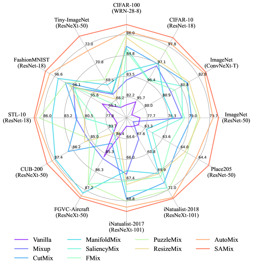
(B) Generalization over datasets. The intuitive performance radar chart presented in Figure 1, combined with the trade-off results in Figure 4, reveals that dynamic mixup methods consistently yield better performance compared to static ones, showcasing their impressive generalizability. However, dynamic approaches necessitate meticulous tuning, which incurs considerable training costs. In contrast, static mixup exhibits significant performance fluctuation across different datasets, indicating poor generalizability with application scenarios. For instance, Mixup and CutMix as the static representatives perform even worse than the baseline on Place205 and FGVC-Aircraft, respectively. Moreover, we analyze how mixup methods improve on different datasets in Figure 6 and Figure A4. On small-scale datasets, mixup methods (dynamic ones) tend to prevent the over-parameterized backbones (Vanilla or with some static ones) from overfitting. On the contrary, mixup techniques are served as data augmentations to encourage the model to fit hard tasks on large-scale datasets.

(C) Generalization over backbones. As shown in Figure 4 and Figure 5(c), we provide extensive evaluations on ImageNet-1K based on different types of backbones and mixup methods. As a result, dynamic mixup achieves better performance in general and shows more favorable generalizability against backbone selection compared to static methods. Noticeably, the online-optimizable SAMix and AutoMix exhibit impressive generalization ability over different vision backbones, which potentially reveals the superiority of their online training framework compared to the others.

(D) Applicability. Figure A2 shows that ViT-specific methods (e.g., TransMix (Chen et al., 2022) and TokenMix (Liu et al., 2022a)) yield exceptional performance with DeiT-S and PVT-S yet exhibit intense sensitivity to different model scales (e.g., with PVT-T). Moreover, they are limited to ViTs, which largely restricts their applicability. Surprisingly, static Mixup (Zhang et al., 2018) exhibits favorable applicability with new efficient networks like MogaNet (Li et al., 2024). CutMix (Yun et al., 2019) fits well with popular backbones, such as modern CNNs (e.g., ConvNeXt and ResNeXt) and DeiT, which increases its applicability. As shown in Figure 4, although AutoMix and SAMix are available in both CNNs and ViTs with consistent superiority, they have limitations in GPU memory and training time, which may limit their applicability in certain cases. This also provides a promising avenue for reducing the cost of well-performed online learnable mixup augmentation algorithms.

(E) Robustness & Calibration. We evaluate the robustness with accuracy on the corrupted version of CIFAR-100 and FGSM attack (Goodfellow et al., 2015) and the prediction calibration. Table A8 shows that all the benchmarked methods can improve model robustness against corruptions. However, only four recent dynamic approaches exhibit improved robustness compared to the baseline with FGSM attacks. We thus hypothesize that the online-optimizable mixup methods are robust against human interference, while the hand-crafted ones adapt to natural disruptions like corruption but are susceptible to attacks. Overall, AutoMix and SAMix achieve the optimal robustness and calibration results. For scenarios where these properties are required, practitioners can prioritize these methods.

(F) Convergence & Training Stability. As shown in Figure 5, wider bump curves indicate smoother loss landscapes (e.g., Mixup), while higher warm color bump tips are associated with better convergence and performance (e.g., AutoMix). Evidently, dynamic mixup algorithms own better training stability and convergence than static mixup in general while obtaining sharp loss landscapes. They are likely to improve performances through exploring hard mixup samples. Nevertheless, the static mixup variants with convex interpolation, especially vanilla Mixup, exhibit smoother loss landscape and stable training than some static cutting-based methods. Based on the observations, we assume this arises from its interpolation that prioritizes training stability but may lead to sub-optimal results.

(G) Downstream Transferability & CAM Visualization. To further evaluate the downstream performance and transferability of different mixup methods, we conduct transfer learning experiments on object detection (Ren et al., 2015), semantic segmentation (Kirillov et al., 2019), and weakly supervised object localization (Choe et al., 2020) with details in Appendix B.4. Notably, Table A11, Table A12, and Table A13 suggest that dynamic sampling mixing methods like AutoMix indeed exhibit competitive results, while recently proposed ViT-specific label mixing methods like TransMix perform even better, showcasing their superior transferability. The results also show the potential for improved online training mixup design. Moreover, it is commonly conjectured that vision models with better CAM localization could potentially be better transferred to fine-grained downstream prediction tasks. As such, to gain intuitive insights, we also provide tools for class activation mapping (CAM) visualization with predicted classes in our codebase. As shown in Figure 7 and Table A13, dynamic mixup like SAMix and AutoMix shows exceptional CAM localization, combined with their aforementioned accuracy, generalization ability, and robustness, may indicate their practical superiority compared to the static ones in object detection and even borader downstream tasks.

5 Conclusion and Discussion

Contributions. This paper presents OpenMixup, the first comprehensive mixup augmentation benchmark and open-source codebase for visual representation learning, where 18 mixup algorithms are trained and thoroughly evaluated on 11 diverse vision datasets. The released codebase not only bolsters the entire benchmark but can facilitate broader under-explored mixup applications and downstream tasks. Furthermore, observations and insights are obtained through different aspects of empirical analysis that are previously under-explored, such as GPU memory usage, loss landscapes, PL exponent alpha metrics, and more, contributing to a deeper and more systematic comprehension of mixup augmentation. We anticipate that our OpenMixup benchmark and codebase can further contribute to fair and reproducible mixup research and we also encourage researchers and practitioners in the community to extend their valuable feedback to us and contribute to OpenMixup for building a more constructive mixup-based visual representation learning codebase together through GitHub.

Limitations and Future Works. The benchmarking scope of this work mainly focuses on visual classification, albeit we have supported a broader range of tasks in the proposed codebase and have conducted transfer learning experiments to object detection and semantic segmentation tasks to draw preliminary conclusions. We are aware of this and have prepared it upfront for future work. For example, our codebase can be easily extended to other computer vision tasks and datasets for further mixup benchmarking experiments and evaluations if necessary. Moreover, our observations and insights can also be of great value to the community for a more comprehensive understanding of mixup augmentation techniques. We believe this work as the first mixup benchmarking study is enough to serve as a kick-start, and we plan to extend our work in these directions in the future.

Acknowledgement

This work was supported by National Key R&D Program of China (No. 2022ZD0115100), National Natural Science Foundation of China Project (No. U21A20427), and Project (No. WU2022A009) from the Center of Synthetic Biology and Integrated Bioengineering of Westlake University. This work was done when Zedong Wang, Juanxi Tian, and Weiyang Jin interned at Westlake University. We sincerely thank Xin Jin for supporting evaluation implementations and all reviewers for polishing our manuscript. We also thank the AI Station of Westlake University for the support of GPUs.

References

Baek et al. (2021) Kyungjune Baek, Duhyeon Bang, and Hyunjung Shim. Gridmix: Strong regularization through local context mapping. Pattern Recognition, 109:107594, 2021.
Berthelot et al. (2019) David Berthelot, Nicholas Carlini, Ian Goodfellow, Nicolas Papernot, Avital Oliver, and Colin A Raffel. Mixmatch: A holistic approach to semi-supervised learning. Advances in Neural Information Processing Systems (NeurIPS), 32, 2019.
Bochkovskiy et al. (2020) Alexey Bochkovskiy, Chien-Yao Wang, and Hong-Yuan Mark Liao. Yolov4: Optimal speed and accuracy of object detection. ArXiv, abs/2004.10934, 2020.
Chattopadhyay et al. (2018) Aditya Chattopadhyay, Anirban Sarkar, Prantik Howlader, and Vineeth N. Balasubramanian. Grad-cam++: Generalized gradient-based visual explanations for deep convolutional networks. 2018 IEEE Winter Conference on Applications of Computer Vision (WACV), pp. 839–847, 2018.
Chen et al. (2022) Jie-Neng Chen, Shuyang Sun, Ju He, Philip Torr, Alan Yuille, and Song Bai. Transmix: Attend to mix for vision transformers. In The IEEE Conference on Computer Vision and Pattern Recognition (CVPR), 2022.
Chen et al. (2019) Kai Chen, Jiaqi Wang, Jiangmiao Pang, Yuhang Cao, Yu Xiong, Xiaoxiao Li, Shuyang Sun, Wansen Feng, Ziwei Liu, Jiarui Xu, Zheng Zhang, Dazhi Cheng, Chenchen Zhu, Tianheng Cheng, Qijie Zhao, Buyu Li, Xin Lu, Rui Zhu, Yue Wu, Jifeng Dai, Jingdong Wang, Jianping Shi, Wanli Ouyang, Chen Change Loy, and Dahua Lin. MMDetection: Open mmlab detection toolbox and benchmark. arXiv preprint arXiv:1906.07155, 2019.
Chen et al. (2023) Mengzhao Chen, Mingbao Lin, Zhihang Lin, Yu xin Zhang, Fei Chao, and Rongrong Ji. Smmix: Self-motivated image mixing for vision transformers. Proceedings of the International Conference on Computer Vision (ICCV), 2023.
Choe et al. (2020) Junsuk Choe, Seong Joon Oh, Seungho Lee, Sanghyuk Chun, Zeynep Akata, and Hyunjung Shim. Evaluating weakly supervised object localization methods right. In Proceedings of the IEEE/CVF Conference on Computer Vision and Pattern Recognition, pp. 3133–3142, 2020.
Choi et al. (2022) Hyeong Kyu Choi, Joonmyung Choi, and Hyunwoo J. Kim. Tokenmixup: Efficient attention-guided token-level data augmentation for transformers. Advances in Neural Information Processing Systems (NeurIPS), 2022.
Chrabaszcz et al. (2017) Patryk Chrabaszcz, Ilya Loshchilov, and Frank Hutter. A downsampled variant of imagenet as an alternative to the cifar datasets. ArXiv, abs/1707.08819, 2017.
Coates et al. (2011) Adam Coates, Andrew Ng, and Honglak Lee. An analysis of single-layer networks in unsupervised feature learning. In Geoffrey Gordon, David Dunson, and Miroslav Dudík (eds.), Proceedings of the Fourteenth International Conference on Artificial Intelligence and Statistics, volume 15 of Proceedings of Machine Learning Research, pp. 215–223, Fort Lauderdale, FL, USA, 11–13 Apr 2011. PMLR.
Contributors (2020a) MMClassification Contributors. Openmmlab’s image classification toolbox and benchmark. https://github.com/open-mmlab/mmclassification, 2020a.
Contributors (2020b) MMSegmentation Contributors. MMSegmentation: Openmmlab semantic segmentation toolbox and benchmark. https://github.com/open-mmlab/mmsegmentation, 2020b.
Dabouei et al. (2021) Ali Dabouei, Sobhan Soleymani, Fariborz Taherkhani, and Nasser M Nasrabadi. Supermix: Supervising the mixing data augmentation. In Proceedings of the IEEE/CVF Conference on Computer Vision and Pattern Recognition (CVPR), pp. 13794–13803, 2021.
Dosovitskiy et al. (2021) Alexey Dosovitskiy, Lucas Beyer, Alexander Kolesnikov, Dirk Weissenborn, Xiaohua Zhai, Thomas Unterthiner, Mostafa Dehghani, Matthias Minderer, Georg Heigold, Sylvain Gelly, Jakob Uszkoreit, and Neil Houlsby. An image is worth 16x16 words: Transformers for image recognition at scale. In International Conference on Learning Representations (ICLR), 2021.
Faramarzi et al. (2020) Mojtaba Faramarzi, Mohammad Amini, Akilesh Badrinaaraayanan, Vikas Verma, and Sarath Chandar. Patchup: A regularization technique for convolutional neural networks, 2020.
Goodfellow et al. (2015) Ian J. Goodfellow, Jonathon Shlens, and Christian Szegedy. Explaining and harnessing adversarial examples. In International Conference on Learning Representations (ICLR), 2015.
ha Lee et al. (2020) Jin ha Lee, M. Zaheer, M. Astrid, and Seung-Ik Lee. Smoothmix: a simple yet effective data augmentation to train robust classifiers. 2020 IEEE/CVF Conference on Computer Vision and Pattern Recognition Workshops (CVPRW), pp. 3264–3274, 2020.
Harris et al. (2020) Ethan Harris, Antonia Marcu, Matthew Painter, Mahesan Niranjan, Adam Prügel-Bennett, and Jonathon S. Hare. Fmix: Enhancing mixed sample data augmentation. arXiv: Learning, 2020.
He et al. (2016) Kaiming He, Xiangyu Zhang, Shaoqing Ren, and Jian Sun. Deep residual learning for image recognition. In Proceedings of the Conference on Computer Vision and Pattern Recognition (CVPR), pp. 770–778, 2016.
He et al. (2017) Kaiming He, Georgia Gkioxari, Piotr Dollár, and Ross Girshick. Mask r-cnn. In Proceedings of the International Conference on Computer Vision (ICCV), 2017.
Hendrycks & Dietterich (2019) Dan Hendrycks and Thomas Dietterich. Benchmarking neural network robustness to common corruptions and perturbations. arXiv preprint arXiv:1903.12261, 2019.
Horn et al. (2018) Grant Van Horn, Oisin Mac Aodha, Yang Song, Yin Cui, Chen Sun, Alex Shepard, Hartwig Adam, Pietro Perona, and Serge Belongie. The inaturalist species classification and detection dataset. In Proceedings of the Conference on Computer Vision and Pattern Recognition (CVPR), 2018.
Kalantidis et al. (2020) Yannis Kalantidis, Mert Bulent Sariyildiz, Noe Pion, Philippe Weinzaepfel, and Diane Larlus. Hard negative mixing for contrastive learning. In Advances in Neural Information Processing Systems (NeurIPS), 2020.
Kim et al. (2020) Jang-Hyun Kim, Wonho Choo, and Hyun Oh Song. Puzzle mix: Exploiting saliency and local statistics for optimal mixup. In International Conference on Machine Learning (ICML), pp. 5275–5285. PMLR, 2020.
Kim et al. (2021) Jang-Hyun Kim, Wonho Choo, Hosan Jeong, and Hyun Oh Song. Co-mixup: Saliency guided joint mixup with supermodular diversity. ArXiv, abs/2102.03065, 2021.
Kirillov et al. (2019) Alexander Kirillov, Ross B. Girshick, Kaiming He, and Piotr Dollár. Panoptic feature pyramid networks. In Proceedings of the Conference on Computer Vision and Pattern Recognition (CVPR), pp. 6392–6401, 2019.
Krizhevsky et al. (2009) Alex Krizhevsky, Geoffrey Hinton, et al. Learning multiple layers of features from tiny images. 2009.
Lewy & Mańdziuk (2023) Dominik Lewy and Jacek Mańdziuk. An overview of mixing augmentation methods and augmentation strategies. Artificial Intelligence Review, pp. 2111–2169, 2023.
Li et al. (2018) Hao Li, Zheng Xu, Gavin Taylor, and Tom Goldstein. Visualizing the loss landscape of neural nets. In Neural Information Processing Systems, 2018.
Li et al. (2021) Siyuan Li, Zicheng Liu, Zedong Wang, Di Wu, Zihan Liu, and Stan Z. Li. Boosting discriminative visual representation learning with scenario-agnostic mixup. ArXiv, abs/2111.15454, 2021.
Li et al. (2024) Siyuan Li, Zedong Wang, Zicheng Liu, Cheng Tan, Haitao Lin, Di Wu, Zhiyuan Chen, Jiangbin Zheng, and Stan Z. Li. Moganet: Multi-order gated aggregation network. In International Conference on Learning Representations (ICLR), 2024.
Lin et al. (2014) Tsung-Yi Lin, Michael Maire, Serge Belongie, James Hays, Pietro Perona, Deva Ramanan, Piotr Dollár, and C Lawrence Zitnick. Microsoft coco: Common objects in context. In Proceedings of the European Conference on Computer Vision (ECCV), 2014.
Liu et al. (2022a) Jihao Liu, B. Liu, Hang Zhou, Hongsheng Li, and Yu Liu. Tokenmix: Rethinking image mixing for data augmentation in vision transformers. Proceedings of the European Conference on Computer Vision (ECCV), 2022a.
Liu et al. (2021) Ze Liu, Yutong Lin, Yue Cao, Han Hu, Yixuan Wei, Zheng Zhang, Stephen Lin, and Baining Guo. Swin transformer: Hierarchical vision transformer using shifted windows. In International Conference on Computer Vision (ICCV), 2021.
Liu et al. (2022b) Zhuang Liu, Hanzi Mao, Chao-Yuan Wu, Christoph Feichtenhofer, Trevor Darrell, and Saining Xie. A convnet for the 2020s. Proceedings of the IEEE/CVF Conference on Computer Vision and Pattern Recognition (CVPR), 2022b.
Liu et al. (2022c) Zicheng Liu, Siyuan Li, Ge Wang, Cheng Tan, Lirong Wu, and Stan Z. Li. Decoupled mixup for data-efficient learning. ArXiv, abs/2203.10761, 2022c.
Liu et al. (2022d) Zicheng Liu, Siyuan Li, Di Wu, Zhiyuan Chen, Lirong Wu, Jianzhu Guo, and Stan Z. Li. Automix: Unveiling the power of mixup for stronger classifiers. Proceedings of the European Conference on Computer Vision (ECCV), 2022d.
Loshchilov & Hutter (2016) Ilya Loshchilov and Frank Hutter. Sgdr: Stochastic gradient descent with warm restarts. arXiv preprint arXiv:1608.03983, 2016.
Loshchilov & Hutter (2019) Ilya Loshchilov and Frank Hutter. Decoupled weight decay regularization. In International Conference on Learning Representations (ICLR), 2019.
Maji et al. (2013) Subhransu Maji, Esa Rahtu, Juho Kannala, Matthew B. Blaschko, and Andrea Vedaldi. Fine-grained visual classification of aircraft. arXiv preprint arXiv:1306.5151, 2013.
Martin et al. (2021) Charles H Martin, Tongsu Peng, and Michael W Mahoney. Predicting trends in the quality of state-of-the-art neural networks without access to training or testing data. Nature Communications, 12(1):4122, 2021.
Muhammad & Yeasin (2020) Mohammed Bany Muhammad and Mohammed Yeasin. Eigen-cam: Class activation map using principal components. 2020 International Joint Conference on Neural Networks (IJCNN), pp. 1–7, 2020.
Naseer et al. (2021) Muhammad Muzammal Naseer, Kanchana Ranasinghe, Salman H Khan, Munawar Hayat, Fahad Shahbaz Khan, and Ming-Hsuan Yang. Intriguing properties of vision transformers. In Advances in Neural Information Processing Systems (NeurIPS), 2021.
Naveed (2021) Humza Naveed. Survey: Image mixing and deleting for data augmentation. ArXiv, abs/2106.07085, 2021.
Paszke et al. (2019) Adam Paszke, Sam Gross, Francisco Massa, Adam Lerer, James Bradbury, Gregory Chanan, Trevor Killeen, Zeming Lin, Natalia Gimelshein, Luca Antiga, Alban Desmaison, Andreas Köpf, Edward Yang, Zach DeVito, Martin Raison, Alykhan Tejani, Sasank Chilamkurthy, Benoit Steiner, Lu Fang, Junjie Bai, and Soumith Chintala. Pytorch: An imperative style, high-performance deep learning library. In Advances in Neural Information Processing Systems (NeurIPS), 2019.
Qin et al. (2024) Huafeng Qin, Xin Jin, Yun Jiang, Mounim A. El-Yacoubi, and Xinbo Gao. Adversarial automixup. In International Conference on Learning Representations (ICLR), 2024.
Qin et al. (2023) Jie Qin, Jiemin Fang, Qian Zhang, Wenyu Liu, Xingang Wang, and Xinggang Wang. Resizemix: Mixing data with preserved object information and true labels. Computational Visual Media (CVMJ), 2023.
Ren et al. (2015) Shaoqing Ren, Kaiming He, Ross B. Girshick, and Jian Sun. Faster r-cnn: Towards real-time object detection with region proposal networks. IEEE Transactions on Pattern Analysis and Machine Intelligence (TPAMI), 39:1137–1149, 2015.
Russakovsky et al. (2015) Olga Russakovsky, Jia Deng, Hao Su, Jonathan Krause, Sanjeev Satheesh, Sean Ma, Zhiheng Huang, Andrej Karpathy, Aditya Khosla, Michael S. Bernstein, Alexander C. Berg, and Li Fei-Fei. Imagenet large scale visual recognition challenge. International Journal of Computer Vision (IJCV), pp. 211–252, 2015.
Sandler et al. (2018) Mark Sandler, Andrew Howard, Menglong Zhu, Andrey Zhmoginov, and Liang-Chieh Chen. Mobilenetv2: Inverted residuals and linear bottlenecks. In Proceedings of the IEEE Conference on Computer Vision and Pattern Recognition (CVPR), 2018.
Selvaraju et al. (2019) Ramprasaath R. Selvaraju, Michael Cogswell, Abhishek Das, Ramakrishna Vedantam, Devi Parikh, and Dhruv Batra. Grad-cam: Visual explanations from deep networks via gradient-based localization. arXiv preprint arXiv:1610.02391, 2019.
Shen et al. (2022) Zhiqiang Shen, Zechun Liu, Zhuang Liu, Marios Savvides, Trevor Darrell, and Eric Xing. Un-mix: Rethinking image mixtures for unsupervised visual representation learning. 2022.
Song et al. (2023) Zifan Song, Xiao Gong, Guosheng Hu, and Cairong Zhao. Deep perturbation learning: enhancing the network performance via image perturbations. In International Conference on Machine Learning, pp. 32273–32287. PMLR, 2023.
Tan & Le (2019) Mingxing Tan and Quoc V. Le. Efficientnet: Rethinking model scaling for convolutional neural networks. In International Conference on Machine Learning (ICML), 2019.
Touvron et al. (2021) Hugo Touvron, Matthieu Cord, Matthijs Douze, Francisco Massa, Alexandre Sablayrolles, and Herve Jegou. Training data-efficient image transformers & distillation through attention. In International Conference on Machine Learning (ICML), pp. 10347–10357, 2021.
Uddin et al. (2020) AFM Uddin, Mst Monira, Wheemyung Shin, TaeChoong Chung, Sung-Ho Bae, et al. Saliencymix: A saliency guided data augmentation strategy for better regularization. arXiv preprint arXiv:2006.01791, 2020.
Venkataramanan et al. (2022) Shashanka Venkataramanan, Yannis Avrithis, Ewa Kijak, and Laurent Amsaleg. Alignmix: Improving representation by interpolating aligned features. Proceedings of the Conference on Computer Vision and Pattern Recognition (CVPR), 2022.
Verma et al. (2019) Vikas Verma, Alex Lamb, Christopher Beckham, Amir Najafi, Ioannis Mitliagkas, David Lopez-Paz, and Yoshua Bengio. Manifold mixup: Better representations by interpolating hidden states. In International Conference on Machine Learning (ICML), 2019.
Wah et al. (2011) Catherine Wah, Steve Branson, Peter Welinder, Pietro Perona, and Serge J. Belongie. The caltech-ucsd birds-200-2011 dataset. California Institute of Technology, 2011.
Walawalkar et al. (2020) Devesh Walawalkar, Zhiqiang Shen, Zechun Liu, and Marios Savvides. Attentive cutmix: An enhanced data augmentation approach for deep learning based image classification. ICASSP 2020 - 2020 IEEE International Conference on Acoustics, Speech and Signal Processing (ICASSP), pp. 3642–3646, 2020.
Wang et al. (2021) Wenhai Wang, Enze Xie, Xiang Li, Deng-Ping Fan, Kaitao Song, Ding Liang, Tong Lu, Ping Luo, and Ling Shao. Pyramid vision transformer: A versatile backbone for dense prediction without convolutions. In IEEE/CVF International Conference on Computer Vision (ICCV), pp. 548–558, 2021.
Wightman et al. (2021) Ross Wightman, Hugo Touvron, and Hervé Jégou. Resnet strikes back: An improved training procedure in timm, 2021.
Wu et al. (2022) Di Wu, Siyuan Li, Zelin Zang, and Stan Z Li. Exploring localization for self-supervised fine-grained contrastive learning. In Proceedings of the British Machine Vision Conference (BMVC), 2022.
Wu et al. (2019) Yuxin Wu, Alexander Kirillov, Francisco Massa, Wan-Yen Lo, and Ross Girshick. Detectron2. https://github.com/facebookresearch/detectron2, 2019.
Xiao et al. (2017) Han Xiao, Kashif Rasul, and Roland Vollgraf. Fashion-mnist: a novel image dataset for benchmarking machine learning algorithms. ArXiv, abs/1708.07747, 2017. URL https://api.semanticscholar.org/CorpusID:702279.
Xie et al. (2017) Saining Xie, Ross Girshick, Piotr Dollár, Zhuowen Tu, and Kaiming He. Aggregated residual transformations for deep neural networks. In Proceedings of the IEEE conference on computer vision and pattern recognition (CVPR), pp. 1492–1500, 2017.
Yun et al. (2019) Sangdoo Yun, Dongyoon Han, Seong Joon Oh, Sanghyuk Chun, Junsuk Choe, and Young Joon Yoo. Cutmix: Regularization strategy to train strong classifiers with localizable features. 2019 IEEE/CVF International Conference on Computer Vision (ICCV), pp. 6022–6031, 2019.
Zagoruyko & Komodakis (2016) Sergey Zagoruyko and Nikos Komodakis. Wide residual networks. In Proceedings of the British Machine Vision Conference (BMVC), 2016.
Zhang et al. (2018) Hongyi Zhang, Moustapha Cissé, Yann Dauphin, and David Lopez-Paz. mixup: Beyond empirical risk minimization. ArXiv, abs/1710.09412, 2018.
Zhao et al. (2023) Qihao Zhao, Yangyu Huang, Wei Hu, Fan Zhang, and Jun Liu. Mixpro: Data augmentation with maskmix and progressive attention labeling for vision transformer. arXiv preprint arXiv:2304.12043, 2023.
Zhou et al. (2014) Bolei Zhou, Agata Lapedriza, Jianxiong Xiao, Antonio Torralba, and Aude Oliva. Learning deep features for scene recognition using places database. In Advances in Neural Information Processing Systems (NeurIPS), pp. 487–495, 2014.
Zhou et al. (2018) Bolei Zhou, Hang Zhao, Xavier Puig, Sanja Fidler, Adela Barriuso, and Antonio Torralba. Semantic understanding of scenes through the ade20k dataset. International Journal of Computer Vision (IJCV), 127:302–321, 2018.

Supplement Material

In supplement material, we provide implementation details and full benchmark results of image classification, downstream tasks, and empirical analysis with mixup augmentations implemented in OpenMixup on various datasets.

Appendix A Implementation Details

A.1 Setup OpenMixup

As provided in the supplementary material or the online document, we simply introduce the installation and data preparation for OpenMixup, detailed in “docs/en/latest/install.md”. Assuming the PyTorch environment has already been installed, users can easily reproduce the environment with the source code by executing the following commands:

⬇

conda activate openmixup

pip install openmim

mim install mmcv-full

\# put the source code here

cd openmixup

python setup.py develop \# or "pip install -e ."

Executing the instructions above, OpenMixup will be installed as the development mode, i.e., any modifications to the local source code take effect, and can be used as a python package. Then, users can download the datasets and the released meta files and symlink them to the dataset root ($OpenMixup/data). The codebase is under Apache 2.0 license.

A.2 Training Settings of Image Classification

Large-scale Datasets.

Table A1 illustrates three popular training settings on large-scaling datasets like ImageNet-1K in detail: (1) PyTorch-style (Paszke et al., 2019). (2) DeiT (Touvron et al., 2021). (3) RSB A2/A3 (Wightman et al., 2021). Notice that the step learning rate decay strategy is replaced by Cosine Scheduler (Loshchilov & Hutter, 2016), and ColorJitter as well as PCA lighting are removed in PyTorch-style setting for better performances. DeiT and RSB settings adopt advanced augmentation and regularization techniques for Transformers, while RSB A3 is a simplified setting for fast training on ImageNet-1K. For a fare comparison, we search the optimal hyper-parameter $\alpha$ in $Beta(\alpha,\alpha)$ from $\{0.1,0.2,0.5,1,2,4\}$ for compared methods while the rest of the hyper-parameters follow the original papers.

Table A1: Ingredients and hyper-parameters used for ImageNet-1K training settings.

Procedure	PyTorch	DeiT	RSB A2	RSB A3
Train Res	224	224	224	160
Test Res	224	224	224	224
Test crop ratio	0.875	0.875	0.95	0.95
Epochs	100/300	300	300	100
Batch size	256	1024	2048	2048
Optimizer	SGD	AdamW	LAMB	LAMB
LR	0.1	$1\times 10^{-3}$	$5\times 10^{-3}$	$8\times 10^{-3}$
LR decay	cosine	cosine	cosine	cosine
Weight decay	$10^{-4}$	0.05	0.02	0.02
Warmup epochs	✗	5	5	5
Label smoothing $\epsilon$	✗	0.1	✗	✗
Dropout	✗	✗	✗	✗
Stoch. Depth	✗	0.1	0.05	✗
Repeated Aug	✗	✓	✓	✗
Gradient Clip.	✗	1.0	✗	✗
H. flip	✓	✓	✓	✓
RRC	✓	✓	✓	✓
Rand Augment	✗	9/0.5	7/0.5	6/0.5
Auto Augment	✗	✗	✗	✗
Mixup alpha	✗	0.8	0.1	0.1
Cutmix alpha	✗	1.0	1.0	1.0
Erasing prob.	✗	0.25	✗	✗
ColorJitter	✗	✗	✗	✗
EMA	✗	✓	✗	✗
CE loss	✓	✓	✗	✗
BCE loss	✗	✗	✓	✓
Mixed precision	✗	✗	✓	✓

Small-scale Datasets.

We also provide two experimental settings on small-scale datasets: (a) Following the common setups (He et al., 2016; Yun et al., 2019) on small-scale datasets like CIFAR-10/100, we train 200/400/800/1200 epochs from stretch based on CIFAR version of ResNet variants (He et al., 2016), i.e., replacing the $7\times 7$ convolution and MaxPooling by a $3\times 3$ convolution. As for the data augmentation, we apply RandomFlip and RandomCrop with 4 pixels padding for 32 $\times$ 32 resolutions. The testing image size is 32 $\times$ 32 (no CenterCrop). The basic training settings include: SGD optimizer with SGD weight decay of 0.0001, a momentum of 0.9, a batch size of 100, and a basic learning rate is 0.1 adjusted by Cosine Scheduler (Loshchilov & Hutter, 2016). (b) We also provide modern training settings following DeiT (Touvron et al., 2021), while using $224\times 224$ and $32\times 32$ resolutions for Transformer and CNN architectures. We only changed the batch size to 100 for CIFAR-100 and borrowed other settings the same as DeiT on ImageNet-1K.

Appendix B Mixup Image Classification Benchmarks

B.1 Mixup Benchmarks on ImageNet-1k

PyTorch-style training settings

The benchmark results are illustrated in Table A2. Notice that we adopt $\alpha=0.2$ for some cutting-based mixups (CutMix, SaliencyMix, FMix, ResizeMix) based on ResNet-18 since ResNet-18 might be under-fitted on ImageNet-1k.

Table A2: Top-1 accuracy (%) of image classification based on ResNet variants on ImageNet-1K using PyTorch-style 100-epoch and 300-epoch training procedures.

	Beta	PyTorch 100 epochs					PyTorch 300 epochs
Methods	$\alpha$	R-18	R-34	R-50	R-101	RX-101	R-18	R-34	R-50	R-101
Vanilla	-	70.04	73.85	76.83	78.18	78.71	71.83	75.29	77.35	78.91
MixUp	0.2	69.98	73.97	77.12	78.97	79.98	71.72	75.73	78.44	80.60
CutMix	1	68.95	73.58	77.17	78.96	80.42	71.01	75.16	78.69	80.59
ManifoldMix	0.2	69.98	73.98	77.01	79.02	79.93	71.73	75.44	78.21	80.64
SaliencyMix	1	69.16	73.56	77.14	79.32	80.27	70.21	75.01	78.46	80.45
FMix	1	69.96	74.08	77.19	79.09	80.06	70.30	75.12	78.51	80.20
ResizeMix	1	69.50	73.88	77.42	79.27	80.55	71.32	75.64	78.91	80.52
PuzzleMix	1	70.12	74.26	77.54	79.43	80.53	71.64	75.84	78.86	80.67
AutoMix	2	70.50	74.52	77.91	79.87	80.89	72.05	76.10	79.25	80.98
AdAutoMix	1	70.86	74.82	78.04	79.91	81.09	-	-	-	-
SAMix	2	70.83	74.95	78.06	80.05	80.98	72.27	76.28	79.39	81.10

Table A3: Top-1 accuracy (%) on ImageNet-1K based on popular Transformer-based architectures using DeiT-S training settings. Notice that

{\dagger}

denotes reproducing results with the official implementation, while other results are implemented with OpenMixup. TransMix, TokenMix, and SMMix are specially designed for Transformers.

Methods	$\alpha$	DeiT-T	DeiT-S	DeiT-B	PVT-T	PVT-S	Swin-T	ConvNeXt-T	MogaNet-T
Vanilla	-	73.91	75.66	77.09	74.67	77.76	80.21	79.22	79.25
DeiT	0.8, 1	74.50	79.80	81.83	75.10	78.95	81.20	82.10	79.02
MixUp	0.2	74.69	77.72	78.98	75.24	78.69	81.01	80.88	79.29
CutMix	0.2	74.23	80.13	81.61	75.53	79.64	81.23	81.57	78.37
ManifoldMix	0.2	-	-	-	-	-	-	80.57	79.07
AttentiveMix+	2	74.07	80.32	82.42	74.98	79.84	81.29	81.14	77.53
SaliencyMix	0.2	74.17	79.88	80.72	75.71	79.69	81.37	81.33	78.74
FMix	0.2	74.41	77.37		75.28	78.72	79.60	81.04	79.05
ResizeMix	1	74.79	78.61	80.89	76.05	79.55	81.36	81.64	78.77
PuzzleMix	1	73.85	80.45	81.63	75.48	79.70	81.47	81.48	78.12
AutoMix	2	75.52	80.78	82.18	76.38	80.64	81.80	82.28	79.43
SAMix	2	75.83	80.94	82.85	76.60	80.78	81.87	82.35	79.62
TransMix	0.8, 1	74.56	80.68	82.51	75.50	80.50	81.80	-	-
TokenMix^†	0.8, 1	75.31	80.80	82.90	75.60	-	81.60	-	-
SMMix	0.8, 1	75.56	81.10	82.90	75.60	81.03	81.80	-	-

Table A4: Top-1 accuracy (%) on ImageNet-1K based on classical ConvNets using RSB A2/A3 training settings, including ResNet, EfficientNet, and MobileNet.V2.

Backbones	$Beta$	R-50	R-50	Eff-B0	Eff-B0	Mob.V2 $1\times$	Mob.V2 $1\times$
Settings	$\alpha$	A3	A2	A3	A2	A3	A2
RSB	0.1, 1	78.08	79.80	74.02	77.26	69.86	72.87
MixUp	0.2	77.66	79.39	73.87	77.19	70.17	72.78
CutMix	0.2	77.62	79.38	73.46	77.24	69.62	72.23
ManifoldMix	0.2	77.78	79.47	73.83	77.22	70.05	72.34
AttentiveMix+	2	77.46	79.34	72.16	75.95	67.32	70.30
SaliencyMix	0.2	77.93	79.42	73.42	77.67	69.69	72.07
FMix	0.2	77.76	79.05	73.71	77.33	70.10	72.79
ResizeMix	1	77.85	79.94	73.67	77.27	69.94	72.50
PuzzleMix	1	78.02	79.78	74.10	77.35	70.04	72.85
AutoMix	2	78.44	80.28	74.61	77.58	71.16	73.19
SAMix	2	78.64	80.40	75.28	77.69	71.24	73.42

DeiT training setting

Table A3 shows the benchmark results following DeiT training setting. Experiment details refer to Sec. A.2. Notice that the performances of transformer-based architectures are more difficult to reproduce than ResNet variants, and the mean of the best performance in 3 trials is reported as their original paper.

RSB A2/A3 training settings

The RSB A2/A3 benchmark results based on ResNet-50, EfficientNet-B0, and MobileNet.V2 are illustrated in Table A4. Training 300/100 epochs with the BCE loss on ImageNet-1k, RSB A3 is a fast training setting, while RSB A2 can exploit the full representation ability of ConvNets. Notice that the RSB settings employ Mixup with $\alpha=0.1$ and CutMix with $\alpha=1.0$ . We report the mean of top-1 accuracy in the last 5/10 training epochs for 100/300 epochs.

B.2 Small-scale Classification Benchmarks

To facilitate fast research on mixup augmentations, we benchmark mixup image classification on CIFAR-10/100 and Tiny-ImageNet with two settings.

CIFAR-10

As elucidated in Sec. A.2, CIFAR-10 benchmarks based on CIFAR version ResNet variants follow CutMix settings, training 200/400/800/1200 epochs from stretch. As shown in Table A5, we report the median of top-1 accuracy in the last 10 training epochs.

Table A5: Top-1 accuracy (%) on CIFAR-10 training 200, 400, 800, 1200 epochs based on ResNet (R) and ResNeXt-32x4d (RX).

Backbones	Beta	R-18	R-18	R-18	R-18	Beta	RX-50	RX-50	RX-50	RX-50
Epochs	$\alpha$	200 ep	400 ep	800 ep	1200ep	$\alpha$	200 ep	400 ep	800 ep	1200ep
Vanilla	-	94.87	95.10	95.50	95.59	-	95.92	95.81	96.23	96.26
MixUp	1	95.70	96.55	96.62	96.84	1	96.88	97.19	97.30	97.33
CutMix	0.2	96.11	96.13	96.68	96.56	0.2	96.78	96.54	96.60	96.35
ManifoldMix	2	96.04	96.57	96.71	97.02	2	96.97	97.39	97.33	97.36
SmoothMix	0.5	95.29	95.88	96.17	96.17	0.2	95.87	96.37	96.49	96.77
AttentiveMix+	2	96.21	96.45	96.63	96.49	2	96.84	96.91	96.87	96.62
SaliencyMix	0.2	96.05	96.42	96.20	96.18	0.2	96.65	96.89	96.70	96.60
FMix	0.2	96.17	96.53	96.18	96.01	0.2	96.72	96.76	96.76	96.10
GridMix	0.2	95.89	96.33	96.56	96.58	0.2	97.18	97.30	96.40	95.79
ResizeMix	1	96.16	96.91	96.76	97.04	1	97.02	97.38	97.21	97.36
PuzzleMix	1	96.42	96.87	97.10	97.13	1	97.05	97.24	97.37	97.34
AutoMix	2	96.59	97.08	97.34	97.30	2	97.19	97.42	97.65	97.51
SAMix	2	96.67	97.16	97.50	97.41	2	97.23	97.51	97.93	97.74

Table A6: Top-1 accuracy (%) on CIFAR-100 training 200, 400, 800, 1200 epochs based on ResNet (R), Wide-ResNet (WRN), ResNeXt-32x4d (RX). Notice that

{\dagger}

denotes reproducing results with the official implementation, while other results are implemented with OpenMixup.

Backbones	Beta	R-18	R-18	R-18	R-18	RX-50	RX-50	RX-50	RX-50	WRN-28-8
Epochs	$\alpha$	200 ep	400 ep	800 ep	1200ep	200 ep	400 ep	800 ep	1200ep	400ep
Vanilla	-	76.42	77.73	78.04	78.55	79.37	80.24	81.09	81.32	81.63
MixUp	1	78.52	79.34	79.12	79.24	81.18	82.54	82.10	81.77	82.82
CutMix	0.2	79.45	79.58	78.17	78.29	81.52	78.52	78.32	77.17	84.45
ManifoldMix	2	79.18	80.18	80.35	80.21	81.59	82.56	82.88	83.28	83.24
SmoothMix	0.2	77.90	78.77	78.69	78.38	80.68	79.56	78.95	77.88	82.09
SaliencyMix	0.2	79.75	79.64	79.12	77.66	80.72	78.63	78.77	77.51	84.35
AttentiveMix+	2	79.62	80.14	78.91	78.41	81.69	81.53	80.54	79.60	84.34
FMix	0.2	78.91	79.91	79.69	79.50	79.87	78.99	79.02	78.24	84.21
GridMix	0.2	78.23	78.60	78.72	77.58	81.11	79.80	78.90	76.11	84.24
ResizeMix	1	79.56	79.19	80.01	79.23	79.56	79.78	80.35	79.73	84.87
PuzzleMix	1	79.96	80.82	81.13	81.10	81.69	82.84	82.85	82.93	85.02
Co-Mixup^†	2	80.01	80.87	81.17	81.18	81.73	82.88	82.91	82.97	85.05
AutoMix	2	80.12	81.78	82.04	81.95	82.84	83.32	83.64	83.80	85.18
SAMix	2	81.21	81.97	82.30	82.41	83.81	84.27	84.42	84.31	85.50
AdAutoMix	1	81.55	81.97	82.32	-	84.40	84.05	84.42	-	85.32

Table A7: Top-1 accuracy (%), GPU memory (G), and total training time (h) of 600 epochs on CIFAR-100 training 200 and 600 epochs based on DeiT-S, Swin-T, and ConvNeXt-T with the DeiT training setting. Notice that all methods are trained on a single A100 GPU to collect training times and GPU memory.

Methods	$\alpha$	DeiT-Small				Swin-Tiny				ConvNeXt-Tiny
		200 ep	600 ep	Mem.	Time	200 ep	600 ep	Mem.	Time	200 ep	600 ep	Mem.	Time
Vanilla	-	65.81	68.50	8.1	27	78.41	81.29	11.4	36	78.70	80.65	4.2	10
Mixup	0.8	69.98	76.35	8.2	27	76.78	83.67	11.4	36	81.13	83.08	4.2	10
CutMix	2	74.12	79.54	8.2	27	80.64	83.38	11.4	36	82.46	83.20	4.2	10
DeiT	0.8, 1	75.92	79.38	8.2	27	81.25	84.41	11.4	36	83.09	84.12	4.2	10
ManifoldMix	2	-	-	8.2	27	-	-	11.4	36	82.06	83.94	4.2	10
SmoothMix	0.2	67.54	80.25	8.2	27	66.69	81.18	11.4	36	78.87	81.31	4.2	10
SaliencyMix	0.2	69.78	76.60	8.2	27	80.40	82.58	11.4	36	82.82	83.03	4.2	10
AttentiveMix+	2	75.98	80.33	8.3	35	81.13	83.69	11.5	43	82.59	83.04	4.3	14
FMix	1	70.41	74.31	8.2	27	80.72	82.82	11.4	36	81.79	82.29	4.2	10
GridMix	1	68.86	74.96	8.2	27	78.54	80.79	11.4	36	79.53	79.66	4.2	10
ResizeMix	1	68.45	71.95	8.2	27	80.16	82.36	11.4	36	82.53	82.91	4.2	10
PuzzleMix	2	73.60	81.01	8.3	35	80.33	84.74	11.5	45	82.29	84.17	4.3	53
AlignMix	1	-	-	-	-	78.91	83.34	12.6	39	80.88	83.03	4.2	13
AutoMix	2	76.24	80.91	18.2	59	82.67	84.05	29.2	75	83.30	84.79	10.2	56
SAMix	2	77.94	82.49	21.3	58	82.70	84.74	29.3	75	83.56	84.98	10.3	57
TransMix	0.8, 1	76.17	79.33	8.4	28	81.33	84.45	11.5	37	-	-	-	-
SMMix	0.8, 1	74.49	80.05	8.4	28	81.55	-	11.5	37	-	-	-	-
Decoupled (DeiT)	0.8, 1	76.75	79.78	8.2	27	81.10	84.59	11.4	36	83.44	84.49	4.2	10

Table A8: More evaluation metric (robustness and calibration) on CIFAR-100 with 200-epoch training, reporting top-1 accuracy (%)

\uparrow

(clean data, corruption data, and FGSM attacks) and calibration ECE (%)

\downarrow

Methods	$\alpha$	DeiT-Small				Swin-Tiny
		Clean	Corruption	FGSM	ECE $\downarrow$	Clean	Corruption	FGSM	ECE $\downarrow$
Vanilla	-	65.81	49.31	20.58	9.48	78.41	58.20	12.87	11.67
Mixup	0.8	69.98	55.85	17.65	7.38	76.78	59.11	15.03	13.89
CutMix	2	74.12	55.08	12.53	6.18	80.64	57.73	18.38	10.95
DeiT	0.8, 1	75.92	57.36	18.55	5.38	81.25	62.21	15.66	15.68
SmoothMix	0.2	67.54	52.42	15.07	30.59	66.69	49.69	9.79	27.10
SaliencyMix	0.2	69.78	51.14	17.31	5.45	80.40	58.43	15.29	10.49
AttentiveMix+	2	75.98	57.57	13.90	9.89	81.13	58.07	15.43	9.60
FMix	1	70.41	51.94	12.20	4.14	80.72	58.44	13.97	9.19
GridMix	1	68.86	51.11	8.43	4.09	78.54	57.78	11.07	9.37
ResizeMix	1	68.45	50.87	20.03	7.64	80.16	57.37	13.64	7.68
PuzzleMix	2	73.60	57.67	17.44	9.45	80.33	60.67	12.96	16.23
AlignMix	1	-	-	-	-	78.91	61.61	17.20	1.92
AutoMix	2	76.24	60.08	27.35	4.69	82.67	64.10	23.62	9.19
SAMix	2	77.94	61.91	30.35	4.01	82.70	62.19	23.66	7.85
TransMix	0.8, 1	76.17	59.89	22.48	8.28	81.33	62.53	18.90	16.47
SMMix	0.8, 1	74.49	59.96	22.85	8.34	81.55	62.86	19.14	16.81
Decoupled (DeiT)	0.8, 1	76.75	59.89	22.48	8.28	81.10	62.25	16.54	16.16

CIFAR-100

As for the classical setting (a), CIFAR-100 benchmarks train 200/400/800/1200 epochs from the stretch in Table A6, similar to CIFAR-10. Notice that we set weight decay to 0.0005 for cutting-based methods (CutMix, AttentiveMix+, SaliencyMix, FMix, ResizeMix) for better performances when using ResNeXt-50 (32x4d) as the backbone. As shown in Table A7 using the modern setting (b), we train three modern architectures for 200/600 epochs from the stretch. We resize the raw images to $224\times 224$ resolutions for DeiT-S and Swin-T while modifying the stem network as the CIFAR version of ResNet for ConvNeXt-T with $32\times 32$ resolutions. As shown in Table A8, we further provided more metrics to evaluate the robustness and reliability (Naseer et al., 2021; Song et al., 2023): evaluating top-1 accuracy on the corrupted version of CIFAR-100 (Hendrycks & Dietterich, 2019), applying FGSM attack (Goodfellow et al., 2015)), and visualizing the prediction calibration (Verma et al., 2019).

Tiny-ImageNet

We largely follow the training setting of PuzzleMix (Kim et al., 2020) on Tiny-ImageNet, which adopts the basic augmentations of RandomFlip and RandomResizedCrop and optimize the models with a basic learning rate of 0.2 for 400 epochs with Cosine Scheduler. As shown in Table A9, all compared methods adopt ResNet-18 and ResNeXt-50 (32x4d) architectures training 400 epochs from the stretch on Tiny-ImageNet.

Backbones	$\alpha$	R-18	RX-50
Vanilla	-	61.68	65.04
MixUp	1	63.86	66.36
CutMix	1	65.53	66.47
ManifoldMix	0.2	64.15	67.30
SmoothMix	0.2	66.65	69.65
AttentiveMix+	2	64.85	67.42
SaliencyMix	1	64.60	66.55
FMix	1	63.47	65.08
GridMix	0.2	65.14	66.53
ResizeMix	1	63.74	65.87
PuzzleMix	1	65.81	67.83
Co-Mixup^†	2	65.92	68.02
AutoMix	2	67.33	70.72
SAMix	2	68.89	72.18
AdAutoMix	1	69.19	72.89

B.3 Downstream Classification Benchmarks

We further provide benchmarks on three downstream classification scenarios in 224 $\times$ 224 resolutions with ResNet architectures, as shown in Table A10.

Benchmarks on Fine-grained Scenarios.

As for fine-grained scenarios, each class usually has limited samples and is only distinguishable in some particular regions. We conduct (a) transfer learning on CUB-200 and FGVC-Aircraft and (b) fine-grained classification with training from scratch on iNat2017 and iNat2018. For (a), we use transfer learning settings on fine-grained datasets, using PyTorch official pre-trained models as initialization and training 200 epochs by SGD optimizer with the initial learning rate of 0.001, the weight decay of 0.0005, the batch size of 16, the same data augmentation as ImageNet-1K settings. For (b) and (c), we follow Pytorch-style ImageNet-1K settings mentioned above, training 100 epochs from the stretch.

Benchmarks on Scenis Scenarios.

As for scenic classification tasks, we study whether mixup augmentations help models distinguish the backgrounds, which are less important than the foreground objects in commonly used datasets. We employ the PyTorch-style training setting like ImageNet-1K on Places205 (Zhou et al., 2014), optimizing models for 100 epochs with SGD optimizer, a basic learning rate of 0.1 with 256 batch size.

Table A10: Top-1 accuracy (%) of mixup image classification with ResNet (R) and ResNeXt (RX) variants on fine-grained datasets (CUB-200, FGVC-Aircraft, iNat2017/2018) and Places205.

	Beta	CUB-200		FGVC-Aircraft		Beta	iNat2017		iNat2018		Beta	Places205
Method	$\alpha$	R-18	RX-50	R-18	RX-50	$\alpha$	R-50	RX-101	R-50	RX-101	$\alpha$	R-18	R-50
Vanilla	-	77.68	83.01	80.23	85.10	-	60.23	63.70	62.53	66.94	-	59.63	63.10
MixUp	0.2	78.39	84.58	79.52	85.18	0.2	61.22	66.27	62.69	67.56	0.2	59.33	63.01
CutMix	1	78.40	85.68	78.84	84.55	1	62.34	67.59	63.91	69.75	0.2	59.21	63.75
ManifoldMix	0.5	79.76	86.38	80.68	86.60	0.2	61.47	66.08	63.46	69.30	0.2	59.46	63.23
SaliencyMix	0.2	77.95	83.29	80.02	84.31	1	62.51	67.20	64.27	70.01	0.2	59.50	63.33
FMix	0.2	77.28	84.06	79.36	86.23	1	61.90	66.64	63.71	69.46	0.2	59.51	63.63
ResizeMix	1	78.50	84.77	78.10	84.0	1	62.29	66.82	64.12	69.30	1	59.66	63.88
PuzzleMix	1	78.63	84.51	80.76	86.23	1	62.66	67.72	64.36	70.12	1	59.62	63.91
AutoMix	2	79.87	86.56	81.37	86.72	2	63.08	68.03	64.73	70.49	2	59.74	64.06
SAMix	2	81.11	86.83	82.15	86.80	2	63.32	68.26	64.84	70.54	2	59.86	64.27

Visualization of Training Stabiltities.

To further analyze training stability and convergence speed, we provided more visualization of the training epoch vs. top-1 validation accuracy of various Mixup augmentations on different datasets to support the conclusion of training convergence, as shown in Figure A3. These visualization results could be easily obtained by our analysis tools under tools/analysis_tools.

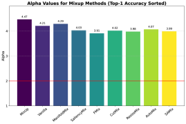
B.4 Transfer Learning

Object Detection.

We conduct transfer learning experiments with pre-trained ResNet-50 (He et al., 2016) and PVT-S (Wang et al., 2021) using mixup augmentations to object detection on COCO-2017 (Lin et al., 2014) dataset, which evaluate the generalization abilities of different mixup approaches. We first fine-tune Faster RCNN (Ren et al., 2015) with ResNet-50-C4 using Detectron2 (Wu et al., 2019) in Table A11, which is trained by SGD optimizer and multi-step scheduler for 24 epochs ( $2\times$ ). The dynamic mixup methods (e.g., AutoMix) usually achieve both competitive performances in classification and object detection tasks. Then, we fine-tune Mask R-CNN (He et al., 2017) by AdamW optimizer for 24 epochs using MMDetection (Chen et al., 2019) in Table A12. We have integrated Detectron2 and MMDetection into OpenMixup, and the users can perform the transferring experiments with pre-trained models and config files. Compared to dynamic sample mixing methods, recently-proposed label mixing policies (e.g., TokenMix and SMMix) yield better performances with less extra training overheads.

Semantic Segmentation.

We also perform transfer learning to semantic segmentation on ADE20K (Zhou et al., 2018) with Semantic FPN (Kirillov et al., 2019) to evaluate the generalization abilities to fine-grained prediction tasks. Following PVT (Wang et al., 2021), we fine-tuned Semantic FPN for 80K interactions by AdamW (Loshchilov & Hutter, 2019) optimizer with the learning rate of $2\times 10^{-4}$ and a batch size of 16 on $512^{2}$ resolutions using MMSegmentation (Contributors, 2020b). Table A12 shows the results of transfer experiments based on PVT-S.

Table A11: Trasfer learning of object detection with ImageNet-1k pre-trained ResNet-50 backbone on COCO dataset.

	IN-1K	COCO
Method	Acc	mAP	AP ${}^{bb}_{50}$	AP ${}^{bb}_{75}$
Vanilla	76.8	38.1	59.1	41.8
Mixup	77.1	37.9	59.0	41.7
CutMix	77.2	38.2	59.3	42.0
ResizeMix	77.4	38.4	59.4	42.1
PuzzleMix	77.5	38.3	59.3	42.1
AutoMix	77.9	38.6	59.5	42.2
SAMix	78.1	38.7	59.6	42.2

Table A12: Trasfer learning of object detection with Mask R-CNN and semantic segmentation with Semantic FPN with pre-trained PVT-S on COCO and ADE20K, respectively.

	IN-1K	COCO			ADE20K
Method	Acc	mAP	AP ${}^{bb}_{50}$	AP ${}^{bb}_{75}$	mIoU
MixUp+CutMix	79.8	40.4	62.9	43.8	41.9
AutoMix	80.7	40.9	63.9	44.1	42.5
TransMix	80.5	40.9	63.8	44.0	42.6
TokenMix	80.6	41.0	64.0	44.3	42.7
TokenMixup	80.5	40.7	63.6	43.9	42.5
SMMix	81.0	41.0	63.9	44.4	43.0

Weakly Supervised Object Localization.

To study the localization ability of trained models more precisely, we follow CutMix (Yun et al., 2019) to evaluate the weakly supervised object localization (WSOL) task on CUB-200 (Wah et al., 2011). The model localizes objects of interest based on the activation maps of CAM (Selvaraju et al., 2019) without bounding box supervision and calculates the maximal box accuracy with a threshold $\delta\in\{0.3,0.5,0.7\}$ as MaxBoxAccV2 (Choe et al., 2020). We provided the benchmarked results on CUB-200 in Table A13, where we found similar conclusions as the visualization of Grad-CAM in Sec. 4.2.

Table A13: MaxBoxAcc (%)

\uparrow

for the Weakly Supervised Object Localization (WSOL) task on CUB-200 based on ResNet architectures. Following CutMix (Yun et al., 2019), the model localizes objects of interest based on the activation maps of CAM (Selvaraju et al., 2019) without bounding box supervision and calculates the maximal box accuracy with a threshold

\delta\in\{0.3,0.5,0.7\}

as MaxBoxAccV2 (Choe et al., 2020).

Backbone	Vanilla	Mixup	CutMix	ManifoldMix	SaliencyMix	FMix	PuzzleMix	Co-Mixup	AutoMix	SAMix
R-18	49.91	48.62	51.85	48.49	52.07	50.30	53.95	54.13	54.46	57.08
RX-50	53.38	50.27	57.16	49.73	58.21	59.80	59.34	59.76	61.05	60.94

B.5 Rules for Counting the Mixup Rankings

We have summarized and analyzed a great number of mixup benchmarking results to compare and rank all the included mixup methods in terms of performance, applicability, and the overall capacity. Specifically, regarding the performance, we averaged the accuracy rankings of all mixup algorithms for each downstream task and averaged their robustness and calibration results rankings separately. Finally, these ranking results are averaged again to produce a comprehensive range of performance ranking results. As for the applicability, we adopt a similar ranking computation scheme considering the time usage and the generalizability of the methods. With the overall capacity ranking, we combined the performance and applicability rankings with a 1:1 weighting to obtain the final take-home rankings. For equivalent results, we take a tied ranking approach. For instance, if three methods are tied for first place, then the method that results in fourth place is recorded as second place by default. Finally, we provide the comprehensive rankings as shown in Table 1 and Table 5.

Appendix C Reproduction Comparison

We provided the reproduction analysis of various mixup methods. Note that AutoMix (Qin et al., 2024), SAMix (Li et al., 2021), AdAutoMix (Qin et al., 2024), and Decouple Mix (Liu et al., 2022c) are originally implemented in OpenMixup, while the other popular mixup algorithms are reproduced based on their official source codes or descriptions. As shown in Table A14 and Table A15, the reproduced results are usually better than the original implementations because of the following reasons: To ensure a fair comparison, we follow the standard training settings for various datasets. Without changing the training receipts, we applied the effective implementations of the basic training components. For example, we employ a better implementation of the cosine annealing learning rate scheduler (updating by iterations) instead of the basic version (updating by epochs). On CIFAR-100, we utilize the RandomCrop augmentation with a “reflect” padding instead of the “zero” padding. On Tiny-ImageNet, we utilize RandomResizedCrop with the cropping ratio of 0.2 instead of RandomCrop in some implementations. On ImageNet-1K, we found that our reproduced results closely align with the reported performances, with any minor discrepancies (around $\pm$ 0.5%) attributable to factors such as random initialization and specific hardware configurations.

Table A14: Comparison of benchmark results reproduced by OpenMixup and the official implementations on CIFAR-100 and Tiny-ImageNet. We report the top-1 accuracy and the training epoch. Note that AutoMix (Qin et al., 2024), SAMix (Li et al., 2021), AdAutoMix (Qin et al., 2024), and Decouple Mix (Liu et al., 2022c) are originally implemented in OpenMixup. The reproduced results are usually better than the original implementations because we applied the effective implementations of the standard training settings without changing the training receipts.

Method	Publication	CIFAR-100 (R18)		Tiny-ImageNet (R18)
		Ours	Official	Ours	Official
MixUp(Zhang et al., 2018)	ICLR’2018	79.24 (1200)	76.84 (1200)	63.86 (400)	58.96 (400)
CutMix(Yun et al., 2019)	ICCV’2019	78.29 (1200)	76.95 (1200)	65.53 (400)	59.89 (400)
SmoothMix(ha Lee et al., 2020)	CVPRW’2020	78.69 (800)	78.14 (800)	66.65 (400)	-
GridMix(Baek et al., 2021)	PR’2020	78.72 (800)	78.09 (800)	64.79 (400)	62.22 (400)
ResizeMix(Qin et al., 2023)	CVMJ’2023	79.19 (400)	79.05 (400)	63.47 (400)	63.23 (400)
ManifoldMix(Verma et al., 2019)	ICML’2019	80.21 (1200)	79.98 (1200)	64.15 (400)	60.24 (400)
FMix(Harris et al., 2020)	arXiv’2020	79.91 (400)	79.85 (400)	63.47 (400)	61.43 (400)
AttentiveMix(Walawalkar et al., 2020)	ICASSP’2020	79.62 (200)	77.16 (200)	64.01 (400)	-
SaliencyMix(Uddin et al., 2020)	ICLR’2021	79.75 (200)	76.11 (200)	64.60 (400)	-
PuzzleMix(Kim et al., 2020)	ICML’2020	81.13 (800)	80.99 (800)	65.81 (400)	63.48 (400)
AlignMixup(Venkataramanan et al., 2022)	CVPR’2022	82.27 (800)	82.12 (800)	66.91 (400)	66.87 (400)

Table A15: Comparison of reproduced results with OpenMixup and the official implementations on ImageNet-1K. We report the top-1 accuracy and the training epoch. Our reproduced results closely align with the reported performances, with any minor discrepancies (around

\pm

0.5%) attributable to factors such as random initialization and specific hardware configurations.

Method	Publication	ImageNet-1K
		Backbone	Ours	Official
MixUp (Zhang et al., 2018)	ICLR’2018	R50	77.12 (100)	77.01 (100)
CutMix (Yun et al., 2019)	ICCV’2019	R50	77.17 (100)	77.08 (100)
SmoothMix (ha Lee et al., 2020)	CVPRW’2020	R50	77.84 (300)	77.66 (300)
GridMix (Baek et al., 2021)	PR’2020	R50	78.50 (300)	78.25 (300)
ResizeMix (Qin et al., 2023)	CVMJ’2023	R50	78.91 (300)	78.90 (300)
ManifoldMix (Verma et al., 2019)	ICML’2019	R50	77.01 (100)	76.85 (100)
FMix (Harris et al., 2020)	arXiv’2020	R50	77.19 (100)	77.03 (100)
AttentiveMix (Walawalkar et al., 2020)	ICASSP’2020	DeiT-S	80.32 (300)	77.50 (300)
SaliencyMix (Uddin et al., 2020)	ICLR’2021	R50	78.46 (300)	78.76 (300)
PuzzleMix (Kim et al., 2020)	ICML’2020	R50	77.54 (100)	77.51 (100)
AlignMixup (Venkataramanan et al., 2022)	CVPR’2022	R50	79.32 (300)	79.50 (300)
TransMix (Chen et al., 2022)	CVPR’2022	DeiT-S	80.80 (300)	80.70 (300)
SMMix (Chen et al., 2023)	ICCV’2023	DeiT-S	81.10 (300)	81.10 (300)