OnsagerNet: Learning Stable and Interpretable Dynamics using a Generalized Onsager Principle
Abstract
We propose a systematic method for learning stable and physically interpretable dynamical models using sampled trajectory data from physical processes based on a generalized Onsager principle. The learned dynamics are autonomous ordinary differential equations parameterized by neural networks that retain clear physical structure information, such as free energy, diffusion, conservative motion and external forces. For high dimensional problems with a low dimensional slow manifold, an autoencoder with metric preserving regularization is introduced to find the low dimensional generalized coordinates on which we learn the generalized Onsager dynamics. Our method exhibits clear advantages over existing methods on benchmark problems for learning ordinary differential equations. We further apply this method to study Rayleigh-Bénard convection and learn Lorenz-like low dimensional autonomous reduced order models that capture both qualitative and quantitative properties of the underlying dynamics. This forms a general approach to building reduced order models for forced dissipative systems.
I Introduction
Discovering mathematical models from observed dynamical data is a scientific endeavor that dates back to the work of Ptolemy, Kepler and Newton. With the recent advancements in machine learning, data-driven approaches have become viable alternatives to those relying purely on human insight. The former has become an active area of research with many proposed methodologies, which can be roughly classified into two categories. The first is unstructured approaches, where the learned dynamics are not a priori constrained to satisfy any physical principles. Instead, minimizing reconstruction error or model complexity are dominant objectives. For example, sparse symbolic regression methods try to find minimal models by searching in a big dictionary of candidate analytic representations [1, 2, 3]; Numerical discretization embedding methods attempt to learn hidden dynamics by embedding known numerical discretization schemes [4, 5, 6]; Galerkin-closure methods use neural networks to reduce the projection error of traditional Galerkin methods [7, 8, 9, 10, 11, 9]. Another line of unstructured methods directly apply time-series modelling tools such as LSTM/GRU and reservoir computing [12, 13, 14] to model temporal evolution of physical processes. For example, it is demonstrated in [12] that reservoir computing can effectively capture the dynamics of high-dimensional chaotic systems, such as the Kuramoto-Sivashinsky equation. These unstructured methods can often achieve high predictive accuracy, but the learned dynamics may not have clear physical structure and theoretical guarantee of temporal stability. This in turn limit their ability to capture qualitative properties of the underlying model on large time intervals. Such issues are significant in that often, the goal of building reduced models is not to reproduce the original dynamics in its entirety, but rather to extract some salient and physically relevant insights. This leads to the second class of structured approaches, where one imparts from the outset some physically motivated constraints to the dynamical system to be learned, e.g. gradient systems [15, 16], Hamiltonian systems [17, 18, 19], etc. These methods have the advantage that the learned models have pre-determined structures and stability may be automatically ensured. However, works in this direction may have the limitation that the structures imposed may be too restrictive to handle complex problems beyond benchmark examples. We demonstrate this point in our benchmark examples to be presented later. It is worth noting that recent works address this issue by a combination of unstructured model fitting with information from an a priori known, but imperfect model, e.g. [20].
In this paper, we propose a systematic method that overcomes the aforementioned limitations. The key idea is a neural network parameterization of a reduced dynamical model, which we call OnsagerNet, based on a highly general extension of the Onsager principle for dissipative dynamics [21, 22]. We choose the Onsager principle, which builds on the second law of thermodynamics and microscopic reversibility, as the starting point due to its simplicity, generality and physical motivation. It naturally gives rise to stable structures for dynamical systems in generalized coordinates, and has been used extensively to derive mathematically well-posed models for complex systems in fluid mechanics, material science, biological science, etc. (see e.g. [23, 24, 25, 26, 27, 28, 29]). However, there are two challenges in using it to find dynamical models with high-fidelity:
-
1.
How to choose the generalized coordinates;
-
2.
How to determine the large amount of free coefficients in the structured dynamical system. Some in-depth discussions could be found in Beris and Edwards [30, Chap 1].
One typical example is the modeling of liquid crystal systems [31, 32]. If the underlying system is near equilibrium, it is possible to determine the coefficients of a reduced-order (macroscopic) model from mathematical analysis or quasi-equilibrium approximations of the underlying microscopic model (see e.g. [33, 34, 35, 36]). Otherwise, this task becomes significantly harder, yet a lot of interesting phenomena happen in this regime. Therefore, a method to derive high fidelity macroscopic models that operate far from equilibrium without a priori scale information is much sought after.
We tackle these two tasks in a data-driven manner. For the first task we learn an approximately isometric embedding to find generalized coordinates. In the linear case this reduces to the principal component analysis (PCA), and in general we modify the autoencoder (AE) [37, 38] with metric preserving regularization designed for trajectory data. For the second task, we avoid the explicit fitting of the prohibitively large number of response coefficients in linearization approaches. Instead, we parameterize nonlinear relationships between generalized coordinates and the physical quantities governing the dynamics (e.g. free energy, dissipation matrices) as neural networks and train them on observed dynamical data with an embedded Runge-Kutta method. The overall approach of OnsagerNet gives rise to stable and interpretable dynamics, yet retaining a degree of generality in the structure to potentially capture complex interactions. By interpretability, we mean that the structure of OnsagerNet parameterization has physical origins, and its learned components can thus be used for subsequent analysis (e.g. visualizing energy landscapes, as shown in Sec. IV). Moreover, we show that the network architecture that we used to parameterize the hidden dynamics has a more general hypothesis space than other existing structured approaches, and can provably represent many dynamical systems with physically meaningful origins (e.g. systems described by generalized Poisson brackets). At the same time, the stability of the OnsagerNet is ensured by its internal structure motivated by physical considerations, and this does not reduce its approximation capacity when applied to dynamical data arising from dissipative processes. We demonstrate the last point by applying the method to the well-known Rayleigh-Bénard convection (RBC) problem, based on which Lorenz discovered a minimal 3-mode ordinary differential equation (ODE) system that exhibits chaos [39]. Lorenz used three dominant modes obtained from linear stability analysis as reduced coordinates and derived the governing equations by a Galerkin projection. As a severely truncated low-dimensional model, the Lorenz model has limited quantitative accuracy when the system is far from the linear stability region. In fact, it is shown by [40] that one needs to use more than 100 modes in a Fourier-Galerkin method to get quantitative accuracy for the 2-dimensional RBC problem that is far from the linear region. In this paper, we show that OnsagerNet is able to learn low dimensional Lorenz-like autonomous ODE models with few modes, yet having high quantitative fidelity to the underlying RBC problem. This validates, and improves upon, the basic approach of Lorenz to capture complex flow phenomena using low dimensional nonlinear dynamics. Furthermore, this demonstrates the effectiveness of a principled combination of physics and machine learning when dealing with data from scientific applications.
II From Onsager principle to OnsagerNet
The Onsager principle [21, 22] is a well-known model for the dynamics of dissipative systems near equilibrium. Given generalized coordinates , their dynamical evolution is modelled by
| (1) |
where is a potential function, typically with a thermodynamic interpretation such as free energy or negated entropy. The matrix models the energy dissipation of the system (or entropy production) and is positive semi-definite in the sense that for all , owing to the second law of thermodynamics. An important result due to Onsager, known as the reciprocal relations, shows that if the system possesses microscopic time reversibility, then is symmetric, i.e. .
The dynamics (1) is simple, yet it can model a large variety of systems close to equilibrium in the linear response regime (see e.g. [41, 24]). However, many dynamical systems in practice are far from equilibrium, possibly sustained by external forces (e.g. the flow induced transition in liquid crystals [33, 34], the kinetic equation with large Knudsen number [42], etc), and in such cases (1) no longer suffices. Thus, it is an important task to generalize or extend (1) to handle these systems.
The extension of known but limited physical principles to more general domains have been a continual exercise in the development of theoretical physics. In fact, (1) itself can be viewed as a generalization of the Rayleigh’s phenomenological principle of least dissipation for hydrodynamics [43]. While classical non-equilibrium statistical physics has been further developed in many aspects, including the study of transport phenomena via Green-Kubo relations [44, 45] and the relations between fluctuations and entropy production [46], an extension of the dynamical model (1) to model general non-equilibrium systems remains elusive. Furthermore, whether a simple yet general extension with solid physical background exists at all is questionable.
This paper takes a rather different approach. Instead of the possibly arduous tasks of developing a general dynamical theory of non-equilibrium systems from first principles, we seek a data-driven extension of (1). In other words, given a dynamical process to be modelled, we posit that it satisfies some reasonable extension of the usual Onsager principle, and determine its precise form from data. In particular, we define the generalized Onsager principle
| (2) |
where the matrix valued functions (resp. ) maps to symmetric positive semi-definite (resp. anti-symmetric) matrices. The last term is a vector field that represents external forces to the otherwise closed system, and may interact with the system in a nonlinear way. The anti-symmetric term models the conservative part of the system, and together with they greatly extend the degree of applicability of the classical Onsager’s principle.
We will assume is invertible everywhere, and hence can be written as a sum of a symmetric positive semi-definite matrix, denoted by and a skew-symmetric matrix, denoted by (see Theorem 5 in Appendix B for a proof), thus we have an equivalent form for equation (2):
| (3) |
where . We will now work with (3) as it is more convenient.
We remark that the form of the generalized Onsager dynamics (2) is not an arbitrary extension of (1). In fact, the dissipative-conservative decomposition () and dependence on are well motivated from classical dynamics. To arrive at the former, we make the crucial observation that a dynamical system defined by generalized Poisson brackets [30] have precisely this decomposition (See Appendix A). Moreover, such forms also appeared in partial differential equation (PDE) models for complex fluids [25, 47]. Note that general Poisson brackets are required to satisfy the Jacobi identity (see e.g. [30, 48]), but in our approach we do not enforce such a condition. We refer to [49] for a neural network implementation based on the generalized Poisson brackets.
II.1 Generalization of Onsager principle for model reduction
Here, we show that the generalized Onsager principle (2) or its equivalent form (3) is invariant under coordinate transformations and is a suitable structured form for model reduction. In the original Onsager principle [21, 22], the system is assumed to be not far away from the equilibrium, such that the system dissipation takes a quadratic form: , i.e. the matrix is assumed to be constant. In our generalization, we assume is a general function that depends . Here we give some arguments why this is necessary and how it can be obtained if the underlying dynamic is given from the viewpoint of model reduction.
To explain nonlinear extension is necessary, we assume that the underlying high-dimensional dynamics which produces the observed trajectories satisfies the form of the generalized Onsager principle with constant and . The dynamics described by an underlying PDE after spatial semi-discretization takes the form
| (4) |
where is a symmetric positive semi-definite constant matrix, is an anti-symmetric matrix. For the dynamics to make sense, we need to be invertible. is a column vector of length . By taking inner product of (4) with , we have an energy dissipation relation of form
Now, suppose that has a solution in a low-dimensional manifold that could be well described by hidden variables with . Denote the low-dimensional solution as , and plug it into (4), we obtain
Multiplying on both sides of the above equation, we have
So, we obtain the following ODE system with model reduction error :
| (5) |
where
| (6) |
Note that as long as has a full column rank, is invertible, so the ODE system makes sense. Now , and depend on in general if is not a constant matrix. Moreover, if the solutions considered all exist exactly in a low-dimensional manifold, i.e. in the above derivation, then (5) is exact, which means the generalized Onsager principle is invariant to non-singular coordinate transformations.
Remark 1
For underlying dynamics given in the alternative form
| (7) |
We first rewrite it into form (4) as
Then, use same procedure as before to obtain
from which, we obtains a reduced model with error :
| (8) |
where , , , and .
Remark 2
When in (4) are constant, if linear PCA is used for model reduction, in which is a constant matrix, then we have are constants. However, if we consider the incompressible Navier-Stokes equations written in form (4), then and are not constant matrices. We obtain nonlinear coefficients in both formulations for the model reduction problem of incompressible Naiver-Stokes equations.
Note that the presence of state () dependence on all the terms implies that we are not linearizing the system about some equilibrium state, as is usually done in linear response theory. Consequently, the functions and may be complicated functions of , and we will learn them from data by parameterizing them as suitably designed neural networks. In this way, we preserve the physical intuition of non-equilibrium physics (dissipation term , conservative term , potential term and external fields ), yet exploit the flexibility of function approximation using data and learning.
In summary, one can view (2) and (3) both as an extension of the classical Onsager principle to handle systems far from equilibrium, or as a reduction of a high dimensional dynamical system defined by generalized Poisson brackets. Both of these dynamics are highly general in their respective domains of application, and serve as solid foundations on which we build our data-driven methodology.
II.2 Dissipative structure and temporal stability of OnsagerNet
From the mathematical point of view, modeling dynamics using (2) or (3) also has clear advantages, in that the learned system is well-behaved as it evolves through time, unlike unstructured approaches such as dynamic mode decomposition (DMD) (see e.g. [50, 51]) and direct parameterization by neural networks, which may achieve a short time trajectory-wise accuracy, but cannot assure mid-to-long time stability as the learned system evolves in time. In our case, we can show in the following result that under mild conditions, the dynamics described by (2) or (3) automatically ensures a dissipative structure, and remains stable as the system evolves in time.
Theorem 1
The solutions to the system (3) satisfy an energy evolution law
| (9) |
If we assume further that there exist positive constants and non-negative constants such that (uniformly positive dissipation), (coercive potential) and (external force has linear growth). Then, for all . In particular, if there is no external force, then is non-increasing in .
Proof Equation (9) can be obtained by pairing both sides of equation (3) with . We now prove boundedness. Using Young’s inequality, we have for any ,
Putting the above estimate with back to (9), to get
By Grönwall inequality, we obtain
where . Finally, by the assumption , is bounded. Note that when , we have , so the above inequality is reduced to , which can be obtained directly from (9) without the requirement of .
Theorem 1 shows that the dynamics is physical under the assumed conditions and we will design our neural network parameterization so that these conditions are satisfied.
III The OnsagerNet architecture and learning algorithm
In this section, we introduce the detailed network architecture for the parameterization of the generalized Onsager dynamics, and discuss the details of the training algorithm.
III.1 Network architecture
We implement the generalized Onsager principle based on equation (3). , , and are represented by neural networks with shared hidden layers and are combined according to (3). The resulting composite network is named OnsagerNet. Accounting for (anti-)symmetry, the numbers of independent variables in , are , , and , respectively.
One important fact is that , as an energy function, should be lower bounded. To ensure this automatically, one may define , where is some constant that is smaller than or equal to ’s lower bound. Since the constant does not affect the dynamics, we drop it in numerical implementation. The actual form we take is
| (10) |
where is a positive hyper-parameter as assumed in Theorem 1 for forced systems. has a similar structure as one component of . We use terms in the form (10) to ensure that an original quadratic energy after a dimension reduction can be handled easily. To see this, suppose the potential function for the high-dimensional problem (with coordinates ) is defined as with symmetric positive definite. Further, let a linear PCA be used for dimensionality reduction. Then, , where . Hence, with representing the matrix , a constant suffices to fully represent quadratic potentials. The autograd mechanism implemented in PyTorch [52] is used to calculate .
To ensure the positive semi-definite property of , we let , where is a lower triangular matrix, is the identity matrix, . Note that the degree of freedom of and can be combined into one matrix, whose upper triangular part determines . A standard multi-layer perception neural network with residual network structure (ResNet) [53] is used to generate adaptive bases, which takes as input, and outputs as linear combinations of those bases. The external force are parameterized based on a priori information, and should be of limited capacity so as not to dilute the physical structures imposed by the other terms. For forced systems considered in this paper, we typically take as affine functions of . The final output of the OnsagerNet is given by
| (11) |
where is defined by (10). Note that in an unforced system we have , since they are only introduced in forced system to ensure a stability of the learned system as required by Theorem 1. The computation procedure of OnsagerNet is described in Architecture 1. The full architecture is summarized in Fig. 1.
Input:
, parameters , activation function ,
number of hidden layer and number of nodes in each hidden layer:
Output:


III.2 Training objective and algorithm
To learn ODE model represented by OnsagerNet based on sampled ODE trajectory data, we minimize following loss function
| (12) |
Here is the time interval of sample data. is the sample set. stands for a second order Runge-Kutta method (Heun method). is the number of steps used to forward the solution of OnsagerNet from snapshots at to . Other Runge-Kutta method can be used. For simplicity, we only present results using Heun method in this paper. This Runge-Kutta embedding method has several advantages over the linear multi-step methods [5, 6], e.g. the variable time interval case and long time interval case can be easily handled by Runge-Kutta methods.
With the definition of the loss function and model architecture, we can then use standard stochastic gradient algorithms to train the network. Here we will use the Adam optimizer [54, 55] to minimize the loss function with a learning rate scheduler that halves the learning rate if the loss is not decreasing in certain numbers of iterations.
III.3 Reduced order model via embedding
The previous section describes the situation when no dimensionality reduction is sought or required, and an Onsager dynamics is learned directly on the original trajectory coordinates. On the other hand, if the data are generated from a numerical discretization of some PDE or a large ODE system, and we want to learn a small reduced order model, then a dimensionality reduction procedure is needed. One can either use linear principal component analysis (PCA) or nonlinear embedding, e.g. the autoencoder, to find a set of good latent coordinates from the high dimensional data. When PCA is used, we perform PCA and OnsagerNet training separately. When an autoencoder is used, we can train it either separately or together with the OnsagerNet. The end-to-end training loss function is taken as
| (13) |
where , stands for the encoder function and decoder function of the autoencoder, respectively. In the last term, is an estimate of the isometric loss (i.e. deviation from being an isometry) of the encoder function based on trajectory data, with being a constant smaller than the average isometric loss of the PCA dimension reduction. Here, stands for positive part and is a penalty constant. is a parameter to balance the autoencoder accuracy and OnsagerNet fitting accuracy.
The choice of autoencoder architecture follows from our observation that PCA performed respectably on a number of examples we studied. Thus, we build the autoencoder by extending the basic PCA. The resulting architecture, which we call PCA-ResNet, is a stacked architecture with each layer consisting of a fully connected autoencoder block with a PCA-type short-cut connection:
| (14) |
where and is a PCA transform from dimension to dimension. is a smooth activation function. The parameters , in the encoder are initialized close to zero, such that the encoder becomes a small perturbation of the PCA. On can regard such an autoencoder as a nonlinear extension of PCA. The decoder is designed similarly. We note that there was a similar but different autoencoder proposed to find slow variables [56].
IV Applications
In this section, we present various applications of the OnsagerNet approach. We will start with benchmark problems and then proceed to investigate more challenging settings such as the Rayleigh-Bénard convection (RBC) problem.
IV.1 Benchmark problem 1: deterministic damped Langevin equation
Here, we use the OnsagerNet to learn a deterministic damped Langevin equation
| (15) |
The friction coefficient may be a constant or a parameter that depends on . For the potential , we consider two cases:
-
•
Hookean spring
(16) -
•
Pendulum model
(17)
Note that no dimensionality reduction is required here and the coordinate entails the full phase space. The goal of this toy example is to quantify the accuracy and stability of the OnsagerNet, as well as to highlight the interpretability of the learned dynamics.
We normalize the parameter by , i.e. we take . To generate data, we simulate the systems using a third order strong stability preserving Runge-Kutta method [57] for a fixed period of time with initial conditions sampled from . Then, we use OnsagerNet (11) to learn an ODE system by fitting the simulated data.
In particular, we will demonstrate that the energy learned has physical meaning. Note that the energy function in the generalized Onsager principle need not be unique. For example, for the heat equation , both and can serve as an energy functional governing the dynamics, with diffusion operators ( matrix) being and the identity respectively. The linear Hookean model is similar. Let , then
| (18) |
The eigenvalue of the matrix is . When , we always obtain real negative eigenvalues, and the system is over-damped. From equation (18), we may define another energy with dissipative matrix and conservative matrix , respectively. For this system, with any non-singular linear transform could serve as energy, and the corresponding dynamics is
Hence, we use this transformation to align the learned energy before making comparison with the exact energy function.
Let us now present the numerical results. We test two cases: 1) Hookean model with , ; 2) Pendulum model with and . To generate sample data, we simulate the ODE systems to obtain 100 trajectories with uniform random initial conditions . For each trajectory, 100 pairs of snapshots at , are used as sample data. Here is the chosen time period of sampled trajectories. Snapshots from the first 80 trajectories are taken as the training set, while the remaining snapshots are taken as the test set.
We test three different methods for learning dynamics: OnsagerNet, a symplectic dissipative ODE net (SymODEN [17]), and a simple multi-layer perception ODE network (MLP-ODEN) with ResNet structure. To make the numbers of trainable parameters in three ODE nets comparable, we choose and for OnsagerNet, for SymODEN, and MLP-ODEN with 2 hidden layers and each layer has hidden units, such that the total numbers of tunable parameters in OnsagerNet, SymODEN and MLP-ODEN are 120, 137, and 124, correspondingly.
To test the robustness of those networks paired with different activation functions, five activation functions are tested, including ReQU, ReQUr, softplus, sigmoid and . Here, ReQU, defined as if , otherwise 0, is the rectified quadratic unit studied in [58]. Since is not uniformly Lipschitz, we introduce ReQUr as a regularization of ReQU, defined as .
The networks are trained using a new version of Adam [55] with mini-batches of size 200 and initial learning rate . The learning rate is halved if the loss is not decreasing in 25 epochs. The default number of iterations is set to 600 epochs.
For the Hookean case, the mean squared error (MSE) loss on testing set can be reduced to about for all the three ODE nets, depending on different random seeds and activation functions used. For the nonlinear pendulum case, the MSE loss on testing set can be reduced to about for OnsagerNet and for MLP-ODEN, but only for SymODEN, see Fig 2. The reason for the low accuracy of SymODEN is that in the SymODEN, the diffusion matrix is assumed to be a function of general coordinate only [17], but here in the damped pendulum problem, the diffusion term depends on . From the test results presented in Figure 2(a), we see that the results of OnsagerNet are not sensitive to the nonlinear activation functions used. Moreover, 2(b) shows that OnsagerNet has much better long time prediction accuracy. Since the nonlinearities in many practical dynamical systems are of polynomial type, we will mainly use ReQU and ReQUr as activation functions for other numerical experiments in this paper.


In Fig 3 we plot the contours of learned energy functions using OnsagerNet and compare with the exact ground truth total energy function . We observe a clear correspondence up to rotation and scaling for the linear Hookean model case and a scaling of the nonlinear pendulum case. In all cases, the minimum is accurately captured. Note that we used a linear transform to align the learned free energy. After the alignment, the relative -norm error between the learned and physical energy for the two tested cases are and respectively. To verify that the OnsagerNet approach is able to learn non-quadratic potentials, we also test an example with exact double-well type potential and . The relative -norm error between the learned and exact energy is , where a simple - rescaling is used before calculating the numerical error for this example.


In Fig. 4, we plot the trajectories for exact dynamics and learned dynamics with initial values starting from four boundaries of the sample region. We see that the learned dynamics are quantitatively accurate, and the qualitative features of the phase space are also preserved over long times.

IV.2 Benchmark problem 2: the Lorenz ’63 system
The previous oscillator models have simple Hamiltonian structures, so it is plausible that with some engineering one can obtain a special structured model that works well for such systems. In this section, we consider a target nonlinear dynamical system that may not have such a simple structure. Yet, we will show that owing to the flexibility of the generalized Onsager principle, OnsagerNet still performs well. Concretely, we consider the well-known Lorenz system [39]:
| (19) | |||||
| (20) | |||||
| (21) |
where is a geometric parameter, is the Prandtl number, is rescaled Rayleigh number.
The Lorenz system (19)-(21) is a simple autonomous ODE system that produces chaotic solutions, and its bifurcation diagram is well-studied [59, 60]. To test the performance of OnsagerNet, we fix , , and vary as commonly studied in the literature. For the , case, the first (pitchfork) bifurcation of the Lorenz system happens at , followed by a homoclinic explosion at , and then a bifurcation to the Lorenz attractor at . Soon after, the Lorenz attractor becomes the only attractor at (see e.g. [61]). To show that OnsagerNet is able to learn systems with different kinds of attractors and chaotic behavior, we present results for and .
The procedure of generating sample data and training is similar to the previously discussed case of learning Langevin equations, except that here we set , and a linear representation for in OnsagerNet (with and ). This is because the Lorenz system is a forced system. The result for the case is presented in Fig 5. We see that both the trajectories and the stable fixed points and unstable limit cycles can be learned accurately. The results for the case is presented in Fig 6. The largest Lyapunov indices of numerical trajectories (run for sufficient long times) are estimated using a method proposed by [62]. They are all positive, which suggests that the learned ODE system indeed has chaotic solutions.


Finally, we compare OnsagerNet with MLP-ODEN for learning the Lorenz system. The SymODEN method [17] cannot be applied since the Lorenz system is non-Hamiltonian. The OnsagerNets used here has one shared hidden layer with 20 hidden nodes, and the total number of trainable parameters is 356. The MLP-ODEN nets have 2 hidden layers with 16 hidden nodes in each layer, with a total 387 tunable parameters. In Fig. 7, we show the accuracy on the test data set for OnsagerNet and MLP-ODEN using and as activation functions, from which we see OnsagerNet performs much better. To ensure that these results hold across different model configurations, we also tested learning the Lorenz system with larger OnsagerNets and MLP-ODENs with 3 hidden layers with 100 hidden nodes each. Some typical training and testing loss curves are given in Figure 8, from which we see OnsagerNet perform better than MLP-ODEN, and activation function ReQUr peforms better than tanh as activation function.


IV.3 Application to Rayleigh-Bénard convection with fixed parameters
We now discuss the main application of OnsagerNet in this paper, namely learning reduced order models for the 2-dimensional Rayleigh-Bénard convection (RBC) problem, described by the coupled partial differential equations
| (22) | |||
| (23) |
where is the velocity field, the gravitational acceleration, is the unit vector opposite to gravity, the departure of the temperature from the linear temperature profile , . is the depth of the channel between two plates. The constants , and denote, respectively, the coefficient of thermal expansion, the kinematic viscosity, and the thermal conductivity. The system is assumed to be homogeneous in direction, and periodic in direction, with period . The dynamics depends on three non-dimensional parameters: the Prandtl number , the Rayleigh number , and aspect ratio . The critical Rayleigh number to maintain the stability of zero solution is . The terms in (22) and in (23) are external forcing terms. For given divergence-free velocity with no-flux or periodic boundary conditions, the convection operator is skew-symmetric. Thus, the RBC equations satisfy the generalized Onsager principle with potential . Therefore, the OnsagerNet approach, which places the prior that the reduced system also satisfy such a principle, is appropriate in this case. The velocity can be represented by a stream function :
| (24) |
By eliminating pressure, one gets the following equations for and :
| (25) | ||||
| (26) |
The solutions to (25) and (26) have representations in Fourier sine series as
where and since and are real. In the Lorenz system, only 3 most important modes , and are retained, in this case, the solution have following form
| (27) |
| (28) |
The Lorenz ’63 equations (19)-(21) for the evolution of is obtained by a Galerkin approach [39] with time rescaling , the rescaled Rayleigh number . , and is the Prandtl number.
Since Lorenz system is aggressively truncated from the original RBC problem, it is not expected to give quantitatively accurate prediction of the dynamics of the original system when . Some extensions of Lorenz system to dimensions higher than 3 are proposed, e.g. Curry’s 14-dimensional model [63]. But numerical experiments have shown that much large numbers of spectral coefficients need be retained to get quantitatively good results in a Fourier-Galerkin approach [40]. In fact, [40] used more than 100 modes to obtain convergent results for a parameter region similar to , , used by Lorenz. In the following, we show that by using OnsagerNet, we are able to directly learn reduced order models from RBC solution data that are quantitatively accurate and require much fewer modes than the Galerkin projection method.
IV.3.1 Data generation and equation parameters
We use a Legendre-Fourier spectral method to solve the Rayleigh-Bénard convection problem (22)-(23) based on stream function formulation (25)-(26) to generate sample data. To be consistent with the case considered by Lorenz, we use free boundary condition for velocity. A RBC problem is chosen with the following parameters: , , , , , . The corresponding Prandtl number, Rayleigh number are , . The relative Rayleigh number is . In this section, we use OnsagerNet to learn one dynamical model for each fixed value. The results of learning one parametric dynamical model for a wide range of value are given in next subsection. Initial conditions of Lorenz form (27)-(28) are used, where are sampled from Gaussian distribution and rescaled such that , with a constant.
The semi-discretized Legendre-Fourier system is solved using a second order implicit-explicit time marching scheme with time step-size for time units. real Fourier modes are used for direction and Legendre modes for direction. To generate training and testing data, we simulated 100 initial values. The solver outputs 2 snapshots of at for each integer time . The data from the first 80 trajectories are used as training data, while the last 20 trajectories are used as testing data.


To have an estimate of the effective dimension, we first apply PCA to the data. The result for is shown in Fig. 9(a). We observe that 99.7% variance are captured by the first 9 principal components, so we seek a reduced model of comparable dimensions.
IV.3.2 The structure of OnsagerNet
The network parameters are similar to that in learning the Lorenz ODE system. Since the Rayleigh-Bénard convection system is not a closed system, we ensure the stability established in Theorem 1 by taking , . To make Lipschitz, we simply let be an affine function of . We use two common hidden layers (i.e. ) with each layer having hidden nodes for evaluating in OnsagerNet. We use ReQUr as activation function in this application as it gives slight better training results than ReQU. The ReQUr OnsagerNet is trained using the standard Adam optimizer [54] to minimize the loss with one embedded RK2 step. The embedding of multiple RK2 steps improves the accuracy only slightly since the time interval of data set is small, and so the error of RK2 integrator is not the major error in the total loss. The use of multiple hidden layers in OnsagerNet also improves accuracy. Since our purpose is to find small models for the dynamics, thus we only present numerical results of OnsagerNets with two common hidden layers.
IV.3.3 Numerical results for r=28
We now present numerical results of the RBC problem with , , and , a parameter set when used in the Lorenz approximation leads to chaotic solutions, but for the original RBC problems, have only fixed points as attractors. We perform PCA for the sampled data and train OnsagerNets using principal components. The OnsagerNets are trained with batch size 200, initial learning rate and reduced by half if the loss is not decrease in 25 epochs. After the reduced ODE models are learned, we simulate the learned equations using a third order Runge-Kutta method [57] for one time unit with initial conditions taken from the PCA data at , and compare the results to the original PCA data at . To show the learned ODE system is stable, we also simulate the learned ODE models for time units. We summarize the results in Table 1. For comparison, we also present results of MLP-ODEN. We see that OnsagerNets have better long time stability than MLP-ODEN. The huge prediction error in MLP-ODEN PCA model indicates that the MLP-ODEN model learned is not stable. From Table 1, we also observe that the OnsagerNets using only three variables () can give good prediction for the period of one time unit (), but has a large relative error () for long times . By increasing gradually to , both the short time and long time prediction accuracy increase.
| Method&Dim | # Parameters | |||||
|---|---|---|---|---|---|---|
| MLP-ODEN PCA 3 | 983 | 2.63 | 3.37 | 2.32 | 3.51 | 62/3 |
| MLP-ODEN PCA 5 | 4079 | 2.95 | 7.84 | 8.18 | 4.12 | 16/3 |
| MLP-ODEN PCA 7 | 11599 | 6.60 | 2.68 | 3.71 | 4.79 | 7/3 |
| OnsagerNet PCA 3 | 776 | 3.17 | 3.85 | 2.54 | 2.76 | 53/3 |
| OnsagerNet PCA 5 | 3408 | 3.88 | 7.47 | 8.40 | 6.87 | 13/3 |
| OnsagerNet PCA 7 | 10032 | 6.71 | 1.26 | 2.68 | 1.07 | 2/3 |
| OnsagerNet AE 3 | 2.5M (AE) 776 | 4.95 | 1.97 | 5.34 | 9.64 | 16/3 |
| OnsagerNet AE 5 | 2.5M (AE) 3408 | 3.71 | 1.19 | 3.35 | 4.63 | 9/3 |
| OnsagerNet AE 7 | 2.5M (AE) 10032 | 1.46 | 4.88 | 1.48 | 1.93 | 3/3 |
in last column presents the average (over 3 random seeds) number of trajectories (out of 100) in the learned ODE systems that do not converge to the correct final steady states.


Some detailed training and testing losses are given in Figure 10. The gap between train error and testing error indicates that the train data has non-negligible sampling error. But from the curve of testing error shown in Fig 10(a), we see the model is not overfitting. We also observe MLP-ODEN has a much larger training-testing error gap than OnsagerNet.
To clearly visualize the numerical errors with respect to time, we show numerical results of using learned OnsagerNets to simulate one selected trajectory in training set and one in testing set with relatively large errors in Fig. 11. We see that as more and more hidden variables are used, the ODE models learned by OnsagerNets are increasingly accurate, even for long times.
| Method | Dim | ||||
|---|---|---|---|---|---|
| OnsagerNet | =3 | 2.65 | 8.47 | 1.30 | 2.63 |
| OnsagerNet | =5 | 9.29 | 3.73 | 6.91 | 8.46 |
| OnsagerNet | =7 | 3.24 | 1.28 | 1.73 | 3.23 |
| NN | =3 | 9.76 | 1.40 | 1.93 | 1.02 |
| NN | =5 | 1.09 | 1.676 | 2.10 | 1.75 |
| NN | =7 | 1.13 | 1.74 | 2.20 | 2.69 |
| Dim | # Parameters | ||
|---|---|---|---|
| 1131 | 4.15 | 2.09 | |
| 4245 | 1.23 | 3.82 | |
| 15653 | 1.02 | 3.73 |
The results of training OnsagerNet together with a PCA-ResNet autoencoder and regularized by the isometric loss defined in Eq. (13) are also presented Table 1. The autoencoder we used has 2 hidden encode layers and 2 hidden decode layers with ReQUr as activation functions. From Table 1, we see the results are improved in this “Autoencoder + OnsagerNet” approach, especially for models with few hidden variables and short time predictions.
To demonstrate the advantange of PCAResNet for dimensionality reduction, we also carried out additional numerical experiments on using different autoencoders, including a standard stacked autoencoder (SAE), a stacked autoencoder with contractive regularization (CAE), which is a multilayer generalization of the original CAE [38], and the PCAResNet. All three autoencoders use two hidden layers with 128 and 32 nodes respectively. The activation function for PCAResNet is ReQUr, while the activation functions for SAE and CAE are elu. We tested other activation functions including ReLU, softplus, elu, tanh and sigmoid for CAE and SAE, and we found that elu produce the best training results. When training SAE and CAE with OnsagerNet, we first pre-train SAE and CAE, than train OnsagerNet with low-dimensional trajectories produced by pre-trained SAE and CAE, then train the autoencoder and OnsagerNet together in the final step. Note that PCAResNet does not require a pre-train step, since it is initialized by a simple PCA. The performance of the three different autoencoders are reported in Table 4, where the and in equation (13) is related to the parameter and in Table 4 by:
| (29) |
From this table, we observe that PCAResNet produce better long time results than SAE and CAE both with and without isometric regularization. From the numerical results presented in Table 4, we clearly see the benefits of isometric regularization - it reduces overfitting (the ratio between testing MSE and training MSE is much smaller when isometric regularization is used) and improves the long time performance for all the three tested autoencoders. Note that and is used to produce the autoencoder results presented in Table 1.
| Autoencoders | ||||||||
|---|---|---|---|---|---|---|---|---|
| PCAResNet | 1 | 0.0 | 1.99 | 5.25 | 2.64 | 7.53 | 3.21 | 85/5 |
| PCAResNet | 1 | 0.4 | 1.27 | 3.40 | 2.68 | 6.49 | 2.67 | 72/5 |
| PCAResNet | 1 | 0.8 | 4.91 | 1.99 | 4.05 | 5.38 | 1.01 | 27/5 |
| PCAResNet | 1 | 1.2 | 4.00 | 1.70 | 4.25 | 5.14 | 8.64 | 24/5 |
| PCAResNet | 1 | 1.6 | 3.78 | 1.39 | 3.68 | 5.41 | 1.31 | 37/5 |
| PCAResNet | 0 | - | 1.07 | 3.37 | 31.50 | 2.24 | 9.17 | 49/5 |
| SAE | 1 | 0.8 | 6.64 | 3.62 | 5.45 | 4.13 | 2.39 | 92/5 |
| SAE | 0 | - | 3.30 | 2.26 | 68.49 | 6.60 | 1.86 | 96/5 |
| CAE | 1 | 0.8 | 5.58 | 2.80 | 4.09 | 3.99 | 1.62 | 67/5 |
| CAE | 0 | - | 3.45 | 6.41 | 185.80 | 1.37 | 3.26 | 135/5 |
is the number of trajectories (out of 100, averaged over 5 seeds) in the learned ODE system that failed to correct final steady state.
We also carry out a comparison on the PCA trajectory prediction error among the OnsagerNet, Long Short Term Memory (LSTM) recurrent neural network, and nearest neighbor method (NN). Since LSTM is a discrete-time process, it cannot learn an underlying ODE model. Rather, we focus on predictions over fixed time intervals (). On the other hand, given a test initial condition, the NN method simply selects the closest initial condition from the training set and use its associated trajectory as a prediction. The numerical results are given in Table 2 and Table 3. We see OnsagerNet out-performs NN method for all cases except for and prediction time . By using more PCs, the OnsagerNet gives better results, but NN does not. From Table 3, we also observe that LSTM does not give better results by using more PCs. We note that both LSTM and NN can only serve as predictive tools for trajectories but does not give rise to a reduced dynamical model in the form of differential equations.


To get an overview of the vector field that drives the learned ODE system represented by OnsagerNet, we draw 2-dimensional projections of phase portraits following several representative trajectories in Fig. 12, from which we see there are four stable fixed points, two of which have relatively larger attraction basins, the other two have very small attraction basins. We numerically verified they are all linearly stable by checking the eigenvalues of Jacobian matrices of the learned system at those points. The two fixed points with larger attraction basin are very similar to those appearing in the Lorenz system with , which corresponds to the two fixed points resulting from the first pitchfork bifurcation, see, e.g. [61, in Fig 2.1], and Fig. 5.
We also test the learned dynamics using OnsagerNet by simulating 100 new numerical trajectories with random initial conditions in the phase space. We observe that they all have negative Lyapunov exponents, which suggests that the learned dynamics have no chaotic solutions. This result is consistent with the original RBC system, which also does not exhibit chaos at these parameter values. In this sense, OnsagerNet also preserves the qualitative properties of the full dynamics, despite being embedding in a much lower dimensional space.

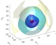
The learned free energy function. In Fig. 13, we show the iso-surfaces of the learned free energy function in the reduced OnsagerNet model for the RBC problem. When PCA data is used, with 3 hidden variables, the free energy learned is irregular, which is very different to a physical free energy function one expect for a smooth dynamical system. As the number of hidden variables is increased, the iso-surfaces of learned free energy function become more and more ellipsoidal, which means the free energy is more akin to a positive definite quadratic form. This is consistent with the exact PDE model. The use of AE in low dimensional case also helps to learn a better free energy function. This again highlights the preservation of physical principles in the OnsagerNet approach.


IV.3.4 A higher Rayleigh number case r=84
For , the RBC problem has only fixed points as attractors. To check the robustness of OnsagerNet to approximate dynamics with different properties, we present results of a higher Rayleigh number case with . The corresponding Rayleigh number is . In this case, the RBC problem has four stable limit cycles. However, starting from initial conditions considered by Lorenz’s reduction, the solution needs to evolve for a very long time to get close to the limit cycles. Thus, whether or not the limit sets are limit cycles are not very clear based on only observations of the sample data. An overview of learned dynamics for is shown in Fig. 14, where four representative trajectories close to the limit cycles together with critical points (saddles) and limit cycles calculated from the learned model are plotted. As before, from this figure we see limit cycles are accurately predicted by reduced order model learned using OnsagerNet. Meanwhile, the saddles can be calculated from the learned OnsagerNet.


A typical trajectory in test set and corresponding results by the learned dynamics are plotted in Fig. 15. These results supports the observation that OnsagerNet achieves both quantitative trajectory accuracy and faithfully captures asymptotic behaviors of the original high-dimensional system.
To check whether the learned reduced order model has chaotic solutions, we carried out a numerical estimate of the largest Lyapunov indices of the trajectories in very long time simulations. Here, we did not find any trajectory with a positive Lyapunov index, which suggest that for the parameter setting used, the RBC problem has no chaotic solution, at least for the type of initial conditions considered in this paper.
IV.4 Application to Rayleigh-Bénard convection in a wide range of Rayleigh number
In this section, we build a reduced model that operates over a wide range of Rayleigh numbers, and hence we sample trajectories corresponding to ten different values in the range . Parameters , , are fixed, and we vary to obtain different values. In all cases, the Prandtl number is fixed at . The data generating procedure is same to the fixed case, but since for multiple case, the dimension of fast manifold is relatively high, we do not use the first 39 pairs of solution snapshots in the trajectories.
The first step is to construct the low-dimensional generalized coordinates using PCA. To account for varying Rayleigh numbers, we perform a common PCA on trajectories with different values. Consequently, we seek an OnsagerNet parameterization with quantities independent of the Rayleigh number . Examining (22)-(23), the dependence may be regarded as strength of the external force, which is linear. Thus, we seek external force of the OnsagerNet as an affine function of . But, different to the fixed case, here we assume is a nonlinear function of .
IV.4.1 Quantitative trajectory accuracy.
We first show that despite being low-dimensional, the learned OnsagerNet preserves trajectory-wise accuracy when compared with the full RBC equations. We summarize the MSE between trajectories generated from the learned OnsagerNet and the true RBC equations for different times in Table 5. Observe that the model using only 7 coordinates () gives good short time () prediction, but has a relatively large error for the long time prediction. By increasing to and , both the short time and long time prediction accuracy increase. We also tested generalization in terms of Rayleigh numbers by withholding data for and testing the learned models in these regimes (Fig. 16). In all cases, the OnsagerNet dynamics remain a quantitatively accurate reduction of the RBC system.
| Dimension | ||||
|---|---|---|---|---|
| =7 | 1.55 | 3.43 | 7.07 | 6.04 |
| =9 | 2.63 | 4.36 | 6.84 | 1.05 |
| =11 | 2.14 | 4.12 | 5.12 | 8.45 |


IV.4.2 Qualitative reproduction of phase space structure.
Next, we show that besides quantitative trajectory accuracy, the qualitative aspects of the RBC, such as long time stability and the nature of the attractor sets, are also adequately captured. This highlights the fact that the approximation power of OnsagerNet does not come at a cost of physical stability and relevance.
To get an overview of the vector field that drives the learned ODE system, we draw 2-dimensional projections of phase portraits for several representative trajectories at in Fig. 16. The data for these Rayleigh numbers are not included in the training set. For the case, we observe four stable fixed points. The two fixed points with larger attraction basins are similar to those appearing in the Lorenz system with , which corresponds to the two fixed points resulting from the first pitchfork bifurcation, see e.g., [61, in Fig 2.1]. Note that the Lorenz ’63 model with is chaotic, but the original RBC problem and our learned model have only fixed points as attractors. For , the four attractors in the RBC problem become more complicated. Starting from Lorenz-type initial conditions, the solutions need to evolve for a very long time to get close to these attractors. The results in Fig. 16 show that the learned low-dimensional models can accurately capture those complicated behavior. Due to the fact that the attractors have larger attraction regions than , we have more type trajectories than type ones. Thus, the vector field near fixed points are learned with higher quantitative accuracy (see Fig. 17), while type trajectory accuracy holds only for short times. Nevertheless, in all cases, the asymptotic qualitative behavior of the trajectories and the attractor sets are faithfully captured.
As motivated earlier, each term in the OnsagerNet parameterization has clear physical origin, and hence once we learn an accurate model, we can study the behavior of each term to infer some physical characteristics of the reduced dynamics. In Fig. 18, we plot the free energy in the learned OnsagerNet model and compare it to the RBC energy function projected to the same reduced coordinates. We observe that the shapes are similar with ellipsoidal iso-surfaces, but the scales vary. This highlights the preservation of physical structure in our approach.

Besides the learned potential, we can also study the diffusion matrix , which measures the rate of energy dissipation as a function of the learned coordinates . In Fig. 19, we plot the eigenvalues of (which characterize dissipation rates along dynamical modes) along the line from point to at , where we observe strong dependence on . This verifies that the OnsagerNet approach is different from linear Galerkin type approximations where the diffusive matrix is constant.

In summary, using the OnsagerNet to learn a reduced model of the RBC equations, we gained two main insights. First, it is possible, under the considered conditions, to obtain an ODE model of relatively low dimension (3-11) that can already capture the qualitative properties (energy functions, attractor sets) while maintaining quantitative reconstruction accuracy for a large range of Rayleigh number. This is in line with Lorenz’ intuition in building the ’63 model. Second, unlike Lorenz highly truncated model, we show that under the parameter settings investigated, the learned OnsagerNet, while having complex dynamics, does not have chaotic behavior.
V Discussion and summary
We have presented a systematic method to construct (reduced) stable and interpretable ODE systems by a machine learning approach based on a generalized Onsager principle. Comparing to existing methods in the literature, our method has several distinct features.
-
•
Comparing to the non-structured machine learning approaches (e.g. [1, 3, 5], etc.), the dynamics learned by our approach have precise physical structure, which not only ensures the stability of the learned models automatically, but also gives physically interpretable quantities, such as free energy, diffusive and conservative terms, etc.
-
•
Comparing to the existing structured approach, e.g. the Lyapunov function approach [15], symplectic structure approach [18, 19], etc., our method, which relies on a principled generalization of the already general Onsager principle, has a more flexible structure incorporating both conservation and dissipation in one equation, which make it suitable for a large class of problems involving forced dissipative dynamics. In particular, the OnsagerNet structure we impose does not sacrifice short-term trajectory accuracy, but still achieves long term stability and qualitative agreement with the underlying dynamics.
- •
-
•
We proposed an isometry-regularized autoencoder to find the slow manifold for given trajectory data for dimension reduction, this is different to traditional feature extraction methods such as proper orthogonal decomposition (POD) [64, 65], dynamic mode decomposition (DMD) and Koopman analysis [50, 66, 51], which only find important linear structures. Our method is also different to the use of an autoencoder with sparse identification of nonlinear dynamics (SINDy) proposed by [67] where sparsity of the dynamics to be learned is used to regularize the autoencoder. The isometric regularization allows the autoencoder to be trained separately or jointly with ODE nets. Moreover, it is usually not easy to ensure long-time stability using these type of methods, especially when the dimension of the learned dynamics increases.
-
•
As a model reduction method, different to the closure approximations approach [7] that based on Mori-Zwanzig theory [68], which needs to work with an explicit mathematical form of underlying dynamical system and usually leads to non-autonomous differential equations, our approach uses only sampled trajectory data to learn autonomous dynamical systems, the learned dynamics can have very good quantitative accuracy and can be readily be further analyzed with traditional ODE analysis methods, or be used as surrogate models for fast online computation.
We have shown the versatility of OnsagerNet by applying it to identify closed and non-closed ODE dynamics: the nonlinear pendulum and Lorenz system with chaotic attractor, and learn reduced order models with high fidelity for the classical meteorological dynamical systems: the Rayleigh-Bénard convection problem.
While versatile, the proposed method can be further improved or extended in several ways. For example, in the numerical results of the RBC problem, we see the accuracy is limited by given sample data when we use enough hidden dimensions. One can use an active sampling strategy (see e.g. [69], [42]) together with OnsagerNet to further improve the accuracy, especially near saddle points. Furthermore, for problems where transient solutions are of interest but lie on a very high-dimensional space, then directly learning PDEs might be a better approach than learning ODE systems. The learning of PDE using OnsagerNet can be accomplished by incorporating the differential operator filter constraints proposed in [4] into its components, e.g. the diffusive and conservative terms. Finally, for problems where sparsity (e.g. memory efficiency) is more important than accuracy, or a balance between these two are needed, one can either add a regularization on the weights of OnsagerNets into the training loss function or incorporate sparse identification methods in the OnsagerNet approach.
Acknowledgments
We would like to thank Prof. Chun Liu, Weiguo Gao, Tiejun Li, Qi Wang, and Dr. Han Wang for helpful discussions. The work of HY and XT are supported by NNSFC Grant 91852116, 11771439 and China Science Challenge Project no. TZ2018001. The work of WE is supported in part by a gift from iFlytek to Princeton University. The work of QL is supported by the start-up grant under the NUS PYP programme. The computations were partially performed on the LSSC4 PC cluster of State Key Laboratory of Scientific and Engineering Computing (LSEC).
Appendix
Appendix A Classical dynamics as generalized Onsager principle
Previously we showed how the dependence arise from projecting high-dimensional dynamics to one on reduced coordinates. There, it is assumed that the high-dimensional dynamics obey the generalized Onsager principle with constant diffusive and conservative terms. Here, we show how this assumption is sensible, by giving general classical dynamical systems that has such a representation.
Theorem 2
Proof The Hamilton equation for given is
Taking , , we have
Theorem 3
Theorem 4
The dynamics described by generalized Poisson brackets, defined below, can be written in form (3). In the Poisson bracket approach, the system is described by generalized coordinates and generalized momentum . Denote the Hamiltonian of the system as . Then, the dynamics of the system is described by the equation [30]
| (31) |
where F is an arbitrary functional depending on the system variables. The reversible and irreversible contributions to the system are represented by the Poisson bracket and the dissipation bracket , respectively, which are defined as
where is symmetric positive semi-definite.
Appendix B Basic properties of non-symmetric positive definite matrices
We present some basic properties of real non-symmetric positive-definite matrices required to show our results.
For a real matrix, we call it positive definite, if there exist a constant , such that , for any . If in the above inequality, we call it positive semi-definite.
For any real matrix , it can be written as a sum of a symmetric part and a skew-symmetric part . For the skew-symmetric part, we have , for any . So a non-symmetric matrix is positive (semi-) positive definite if and only if its symmetric part is positive (semi-)definite.
The following theorem is used in deriving alternative forms of the generalized Onsager dynamics.
Theorem 5
1) Suppose is a positive semi-definite real matrix, then the real parts of its eigenvalues are all non-negative. 2) The inverse of a non-singular positive semi-definite is also positive semi-definite.
Proof Suppose that is an eigenvalue of , the corresponding eigenvector is , then
So
Left multiply the equation by to get (this is the real part of )
If is positive semi-definite, then we obtain , 1) is proved.
Now suppose that positive semi-definite and invertible, then for any we can define by to get
The second part is proved.
Note that the converse of the first part in Theorem 5 is not true. An simple counterexample is , whose eigenvalues are . But the eigenvalues of its symmetric part are .
References
- Bongard and Lipson [2007] J. Bongard and H. Lipson, Automated reverse engineering of nonlinear dynamical systems, Proc. Natl. Acad. Sci. 104, 9943 (2007).
- Schmidt and Lipson [2009] M. Schmidt and H. Lipson, Distilling free-form natural laws from experimental data, Science 324, 81 (2009).
- Brunton et al. [2016] S. L. Brunton, J. L. Proctor, and J. N. Kutz, Discovering governing equations from data by sparse identification of nonlinear dynamical systems, Proc. Natl. Acad. Sci. 113, 3932 (2016).
- Long et al. [2018] Z. Long, Y. Lu, X. Ma, and B. Dong, PDE-Net: Learning PDEs from data, in 35th International Conference on Machine Learning, ICML 2018 (2018) pp. 5067–5078.
- Raissi et al. [2018] M. Raissi, P. Perdikaris, and G. E. Karniadakis, Multistep neural networks for data-driven discovery of nonlinear dynamical systems, ArXiv180101236 (2018), arXiv:1801.01236 .
- Xie et al. [2019a] X. Xie, G. Zhang, and C. G. Webster, Non-intrusive inference reduced order model for fluids using linear multistep neural network, Mathematics 7, 10.3390/math7080757 (2019a), arXiv:1809.07820 [physics] .
- Wan et al. [2018] Z. Y. Wan, P. R. Vlachas, P. Koumoutsakos, and T. P. Sapsis, Data-assisted reduced-order modeling of extreme events in complex dynamical systems, PLoS ONE 13, e0197704 (2018), arXiv:1803.03365 .
- Pan and Duraisamy [2018] S. Pan and K. Duraisamy, Data-driven discovery of closure models, SIAM J. Appl. Dyn. Syst. 17, 2381 (2018).
- Wang et al. [2020] Q. Wang, N. Ripamonti, and J. S. Hesthaven, Recurrent neural network closure of parametric POD-Galerkin reduced-order models based on the Mori-Zwanzig formalism, J. Comput. Phys. 410, 109402 (2020).
- Ma et al. [2019] C. Ma, J. Wang, and W. E, Model reduction with memory and the machine learning of dynamical systems, Commun. Comput. Phys. 25, 10.4208/cicp.OA-2018-0269 (2019).
- Xie et al. [2019b] C. Xie, K. Li, C. Ma, and J. Wang, Modeling subgrid-scale force and divergence of heat flux of compressible isotropic turbulence by artificial neural network, Phys. Rev. Fluids 4, 10.1103/PhysRevFluids.4.104605 (2019b).
- Pathak et al. [2018] J. Pathak, B. Hunt, M. Girvan, Z. Lu, and E. Ott, Model-free prediction of large spatiotemporally chaotic systems from data: A reservoir computing approach, Physical Review Letters 120, 024102 (2018).
- Vlachas et al. [2020] P. R. Vlachas, J. Pathak, B. R. Hunt, T. P. Sapsis, M. Girvan, E. Ott, and P. Koumoutsakos, Backpropagation algorithms and reservoir computing in recurrent neural networks for the forecasting of complex spatiotemporal dynamics, Neural Networks 126, 191 (2020).
- Szunyogh et al. [2020] I. Szunyogh, T. Arcomano, J. Pathak, A. Wikner, B. Hunt, and E. Ott, A Machine-Learning-Based Global Atmospheric Forecast Model, Preprint (Atmospheric Sciences, 2020).
- Kolter and Manek [2019] J. Z. Kolter and G. Manek, Learning stable deep dynamics models, 33rd Conf. Neural Inf. Process. Syst. , 9 (2019).
- Giesl et al. [2020] P. Giesl, B. Hamzi, M. Rasmussen, and K. Webster, Approximation of Lyapunov functions from noisy data, J. Comput. Dyn. 7, 57 (2020).
- Zhong et al. [2020a] Y. D. Zhong, B. Dey, and A. Chakraborty, Symplectic ODE-Net: Learning Hamiltonian dynamics with control, ICLR 2020, ArXiv190912077 (2020a).
- Jin et al. [2020] P. Jin, A. Zhu, G. E. Karniadakis, and Y. Tang, Symplectic networks: Intrinsic structure-preserving networks for identifying Hamiltonian systems, Neural Networks 32, 166 (2020).
- Zhong et al. [2020b] Y. D. Zhong, B. Dey, and A. Chakraborty, Dissipative SymODEN: Encoding Hamiltonian dynamics with dissipation and control into deep learning, arXiv:2002.08860 (2020b).
- Wikner et al. [2020] A. Wikner, J. Pathak, B. Hunt, M. Girvan, T. Arcomano, I. Szunyogh, A. Pomerance, and E. Ott, Combining machine learning with knowledge-based modeling for scalable forecasting and subgrid-scale closure of large, complex, spatiotemporal systems, Chaos: An Interdisciplinary Journal of Nonlinear Science 30, 053111 (2020).
- Onsager [1931a] L. Onsager, Reciprocal relations in irreversible processes. I, Phys. Rev. 37, 405 (1931a).
- Onsager [1931b] L. Onsager, Reciprocal relations in irreversible processes. II, Phys. Rev. 38, 2265 (1931b).
- Qian et al. [2006] T. Qian, X.-P. Wang, and P. Sheng, A variational approach to moving contact line hydrodynamics, J. Fluid Mech. 564, 333 (2006).
- Doi [2011] M. Doi, Onsager’s variational principle in soft matter, J. Phys.: Condens. Matter 23, 284118 (2011).
- Yang et al. [2016] X. Yang, J. Li, M. Forest, and Q. Wang, Hydrodynamic theories for flows of active liquid crystals and the generalized Onsager principle, Entropy 18, 202 (2016).
- Giga et al. [2017] M.-H. Giga, A. Kirshtein, and C. Liu, Variational modeling and complex fluids, in Handbook of Mathematical Analysis in Mechanics of Viscous Fluids, edited by Y. Giga and A. Novotny (Springer International Publishing, Cham, 2017) pp. 1–41.
- Jiang et al. [2019] W. Jiang, Q. Zhao, T. Qian, D. J. Srolovitz, and W. Bao, Application of Onsager’s variational principle to the dynamics of a solid toroidal island on a substrate, Acta Mater. 163, 154 (2019).
- Doi et al. [2019] M. Doi, J. Zhou, Y. Di, and X. Xu, Application of the Onsager-Machlup integral in solving dynamic equations in nonequilibrium systems, Phys Rev E 99, 063303 (2019).
- Xu and Qian [2019] X. Xu and T. Qian, Generalized Lorentz reciprocal theorem in complex fluids and in non-isothermal systems, J. Phys.: Condens. Matter 31, 475101 (2019).
- Beris and Edwards [1994] A. N. Beris and B. Edwards, Thermodynamics of Flowing Systems (Oxford Science Publications, New York, 1994).
- Doi and Edwards [1986] M. Doi and S. F. Edwards, The Theory of Polymer Dynamics (Oxford University Press, USA, 1986).
- De Gennes and Prost [1993] P. G. De Gennes and J. Prost, The Physicsof Liquid Crystals, 2nd ed. (Clarendon Press, 1993).
- Kröger and Ilg [2007] M. Kröger and P. Ilg, Derivation of Frank-Ericksen elastic coefficients for polydomain nematics from mean-field molecular theory for anisotropic particles, J. Chem. Phy. 127, 034903 (2007).
- Yu et al. [2010] H. Yu, G. Ji, and P. Zhang, A nonhomogeneous kinetic model of liquid crystal polymers and its thermodynamic closure approximation, Commun. Comput. Phy. 7, 383 (2010).
- E [2011] W. E, Principles of Multiscale Modeling (Cambridge University Press, New York, 2011).
- Han et al. [2015] J. Han, Y. Luo, W. Wang, P. Zhang, and Z. Zhang, From microscopic theory to macroscopic theory: A systematic study on modeling for liquid crystals, Arch. Rational Mech. Anal. 215, 741 (2015).
- Hinton and Salakhutdinov [2006] G. E. Hinton and R. R. Salakhutdinov, Reducing the dimensionality of data with neural networks, Science 313, 504 (2006).
- Rifai et al. [2011] S. Rifai, P. Vincent, X. Muller, X. Glorot, and Y. Bengio, Contractive auto-encoders: Explicit invariance during feature extraction, Proceedings of the 28th International Conference on Machine Learning , 8 (2011).
- Lorenz [1963] E. N. Lorenz, Deterministic nonperiodic flow, J. Atmos. Sci. 20, 130 (1963).
- Curry et al. [1984] J. H. Curry, J. R. Herring, J. Loncaric, and S. A. Orszag, Order and disorder in two- and three-dimensional Bénard convection, J. Fluid Mech. 147, 1 (1984).
- De Groot and Mazur [1962] S. R. De Groot and P. Mazur, Non-Equilibrium Thermodynamics (Dover Publications, 1962).
- Han et al. [2019] J. Han, C. Ma, Z. Ma, and W. E, Uniformly accurate machine learning-based hydrodynamic models for kinetic equations, Proc. Natl. Acad. Sci. 116, 21983 (2019).
- Rayleigh [1878] L. Rayleigh, On the instability of jets, P. Lond. Math. Soc. s1-10, 4 (1878).
- Green [1954] M. S. Green, Markoff random processes and the statistical mechanics of time-dependent phenomena. II. Irreversible processes in fluids, J. Chem. Phys. 22, 398 (1954).
- Kubo [1957] R. Kubo, Statistical-mechanical theory of irreversible processes. I. General theory and simple applications to magnetic and conduction problems, J. Phys. Soc. Jpn. 12, 570 (1957).
- Evans and Searles [2002] D. J. Evans and D. J. Searles, The fluctuation theorem, Adv. Phys. 51, 1529 (2002).
- Zhao et al. [2018] J. Zhao, X. Yang, Y. Gong, X. Zhao, X. Yang, J. Li, and Q. Wang, A general strategy for numerical approximations of non-equilibrium models–part I: Thermodynamical systems, Int. J. Numer. Anal. Model. 15, 884 (2018).
- Ottinger [2005] H. C. Ottinger, Beyond Equilibrium Thermodynamics (John Wiley & Sons, 2005).
- Hernández et al. [2021] Q. Hernández, A. Badias, D. Gonzalez, F. Chinesta, and E. Cueto, Structure-preserving neural networks, J. Comput. Phy. 426, 109950 (2021).
- Schmid [2010] P. J. Schmid, Dynamic mode decomposition of numerical and experimental data, J. Fluid Mech. 656, 5 (2010).
- Takeishi et al. [2017] N. Takeishi, Y. Kawahara, and T. Yairi, Learning Koopman invariant subspaces for dynamic mode decomposition, in Advances in Neural Information Processing Systems 30 (Curran Associates, Inc., 2017) pp. 1130–1140.
- Paszke et al. [2019] A. Paszke, S. Gross, F. Massa, A. Lerer, J. Bradbury, G. Chanan, T. Killeen, Z. Lin, N. Gimelshein, L. Antiga, A. Desmaison, A. Kopf, E. Yang, Z. DeVito, M. Raison, A. Tejani, S. Chilamkurthy, B. Steiner, L. Fang, J. Bai, and S. Chintala, PyTorch: An imperative style, high-performance deep learning library, in Advances in Neural Information Processing Systems 32 (Curran Associates, Inc., 2019) pp. 8026–8037.
- He et al. [2016] K. He, X. Zhang, S. Ren, and J. Sun, Deep residual learning for image recognition, in Proceedings of the IEEE conference on computer vision and pattern recognition (2016) pp. 770–778.
- Kingma and Ba [2015] D. P. Kingma and J. Ba, Adam: A method for stochastic optimization, in 3rd International Conference for Learning Representations, arXiv:1412.6980 (San Diego, 2015).
- Reddi et al. [2018] S. J. Reddi, S. Kale, and S. Kumar, On the convergence of Adam and beyond, in International Conference on Learning Representations (2018).
- Linot and Graham [2020] A. J. Linot and M. D. Graham, Deep learning to discover and predict dynamics on an inertial manifold, Phys. Rev. E 101, 062209 (2020).
- Shu and Osher [1988] C.-W. Shu and S. Osher, Efficient implementation of essentially non-oscillatory shock-capturing schemes, J. Comput. Phys. 77, 439 (1988).
- Li et al. [2020] B. Li, S. Tang, and H. Yu, Better approximations of high dimensional smooth functions by deep neural networks with rectified power units, Commun. Comput. Phs. 27, 379 (2020).
- Sparrow [1982] C. Sparrow, The Lorenz Equations: Bifurcations, Chaos, and Strange Attractors (Springer-Verlag, New York, 1982).
- Barrio and Serrano [2007] R. Barrio and S. Serrano, A three-parametric study of the Lorenz model, Physica D 229, 43 (2007).
- Zhou and E [2010] X. Zhou and W. E, Study of noise-induced transitions in the Lorenz system using the minimum action method, Commun. Math. Sci. 8, 341 (2010).
- Rosenstein et al. [1993] M. T. Rosenstein, J. J. Collins, and C. J. De Luca, A practical method for calculating largest Lyapunov exponents from small data sets, Physica D 65, 117 (1993).
- Curry [1978] J. H. Curry, A generalized Lorenz system, Commun. Math. Phys. 60, 193 (1978).
- Lumley [1970] J. Lumley, Stochastic Tools in Turbulence (Academic Press, 1970).
- Holmes et al. [1996] P. Holmes, J. Lumley, and G. Berkooz, Turbulence, Coherent Structures, Dynamical Systems and Symmetry (Cambridge Univ Press, 1996).
- Rowley et al. [2009] C. W. Rowley, I. Mezić, S. Bagheri, P. Schlatter, and D. S. Henningson, Spectral analysis of nonlinear flows, J. Fluid Mech. 641, 115 (2009).
- Champion et al. [2019] K. Champion, B. Lusch, J. N. Kutz, and S. L. Brunton, Data-driven discovery of coordinates and governing equations, Proc. Natl. Acad. Sci. 116, 22445 (2019).
- Chorin et al. [2000] A. J. Chorin, O. H. Hald, and R. Kupferman, Optimal prediction and the Mori-Zwanzig representation of irreversible processes, Proc. Natl. Acad. Sci. 97, 2968 (2000).
- Zhang et al. [2019] L. Zhang, D. Y. Lin, H. Wang, R. Car, and W. E, Active learning of uniformly accurate interatomic potentials for materials simulation, Physical Review Materials 3, 023804 (2019).