Only One Relation Possible?
Modeling the Ambiguity in Event Temporal Relation Extraction
Abstract
Event Temporal Relation Extraction (ETRE) aims to identify the temporal relationship between two events, which plays an important role in natural language understanding. Most previous works follow a single-label classification style, classifying an event pair into either a specific temporal relation (e.g., Before, After), or a special label Vague when there may be multiple possible temporal relations between the pair. In our work, instead of directly making predictions on Vague, we propose a multi-label classification solution for ETRE (METRE) to infer the possibility of each temporal relation independently, where we treat Vague as the cases when there is more than one possible relation between two events. We design a speculation mechanism to explore the possible relations hidden behind Vague, which enables the latent information to be used efficiently. Experiments on TB-Dense, MATRES and UDS-T show that our method can effectively utilize the Vague instances to improve the recognition for specific temporal relations and outperforms most state-of-the-art methods.
1 Introduction
Event Temporal Relation Extraction (ETRE) is a task to determine the temporal relationship between two events in a given text, which could benefit many downstream tasks, such as summarization, generation, question answering and so on Ng et al. (2014); Yu et al. (2017); Shi et al. (2019).
According to the ambiguity of the temporal relationship between an event pair, most benchmarks categorize the temporal relationship between events into two types: the well-defined relations Cassidy et al. (2014) and Vague. Well-defined relations indicate the specific temporal relations that can be explicitly positioned in the timeline. For example, TB-Dense Cassidy et al. (2014) contains five well-defined relations: Before, After, Include, Is Included, Simultaneous, while MATRES Ning et al. (2018) have three: Before, After and Equal. As for the special label, Vague, it indicates the cases when people, based on the currently available context, can not make an agreement on which well-defined relation should be chosen for the given event pair. Due to its complexity and ambiguity, how to better characterize Vague and other well-defined relations is still a challenge for ETRE.
| TEXT: My son has fallen asleep , so I have some free time to read for a while. | |
| Possible Scenario 1: | Possible Relation 1 |
| My son woke up while I was reading. | Before |
| Possible Scenario 2: | Possible Relation 2 |
| My son didn’t wake up until I finished reading the book. | Include |
Although recent works have made many attempts to reduce the inconsistency of temporal relation labeling, such as using course relations Verhagen et al. (2007) or setting rules to push annotators to carefully consider Vague Ning et al. (2018), they still pay less attention to why various Vague cases are challenging and how to deal with them better. For example, in Table 1, given the text "My son has fallen asleep, so I have some free time to read for a while.", we can only infer that event "asleep" happening before or include event "read" are both possible, and then determine event pair <asleep, read> as Vague. In other words, Vague can be explained as an event pair with more than one possible temporal relationship between them.
Most previous studies on ETRE ignore the premise that Vague is determined due to the multiple possible well-defined temporal relations between an event pair, and treat Vague independently and equally as other well-defined relations. They formulate ETRE as a single-label classification task, in which they directly predict by choosing the most possible one from all candidate relations. However, such a single-label classification paradigm will cause the model’s confusion between the meaning of Vague and other potentially related well-defined relations. Take the sentence in Table 1 as an example again; the model may capture the information that there is the possibility of event "asleep" happening before event "read", thus wrongly classifying <asleep, read> into Before. On the other hand, after being told that this case should be considered as Vague, the model will punish all features contributing to Before. Unfortunately, doing this will actually confuse the model, since the sentence contains clues for both Before and Include, the reason why annotators label it with Vague.
To address this problem, instead of treating Vague as a single label independent from others, we view Vague as the situation when there is more than one possible well-defined temporal relation between an event pair. We propose a Multi-label Event Temporal Relation Extraction (METRE) method that transforms the task into a multi-label classification style, and makes predictions on every well-defined relation about its possibility being the temporal relation between the given event pair. If more than one relation is of high possibility, we consider the relation between the event pair as Vague. Thus the intrinsic composition of Vague can be properly formulated and make it distinguishable from other well-defined relations.
Experiments on TBDense, MATRES and UDS-T Vashishtha et al. (2019) show METRE could outperform most previous state-of-the-art methods, indicating our model could better characterize and make full use of the special label Vague. Further analysis demonstrates that, instead of the tendency to predict an event pair as Vague, our model predicts more well-defined relations with higher accuracy compared to the baseline model. Consistent improvement in low-data scenarios also shows that we can explore the information hidden behind Vague efficiently. We also show that our method could even find those well-defined relations that possibly cause the Vague annotations, providing further interpretability for the ETRE task.
2 Related Work
Disagreement is widespread during the temporal relation annotation process. Many previous works, such as TempEval-3 UzZaman et al. (2013) and THYME Styler IV et al. (2014), annotate every event pair by at least two annotators, and the final result is obtained with the adjudication of the third annotator. Similarly, MAVEN-ERE Wang et al. (2022b) uses majority voting to produce the final gold standard annotations. These datasets only contain well-defined relations after achieving agreement among annotators. Many studies retain controversial information in the corpus. For example, TB-Dense Cassidy et al. (2014) treat the relation between an event pair as Vague if more than half of the annotators disagree on certain well-defined relations, while Verhagen et al. (2007) and MATRES Ning et al. (2018) directly provide relation Vague for each annotator to choose. Differently, UDS-T Vashishtha et al. (2019) preserves the detailed annotation results of every annotator and flexible rules of the disagreement adjudication can be applied to it.
The ambiguity of Vague is often neglected in ETRE. Previous studies on temporal relation extraction are mainly formulated as a single-label classification task, overlooking the intrinsic nature of Vague and treating every relation equally. They pay attention to the essential context information extraction and are looking forward to obtaining a better event pair representation. With the rapid development of pre-trained language models, most recent works Han et al. (2019); Wang et al. (2020) adopt BERT Devlin et al. (2019) or RoBERTa Liu et al. (2019) to obtain contextualized representations for event pairs. Besides, several researchers Meng et al. (2017); Cheng and Miyao (2017); Zhang et al. (2022) notice the importance of syntactic features, e.g., Part-Of-Speech tags, dependency parses, etc., and incorporate them into the model. Recent studies try to model temporal relations by taking their definitions and properties into consideration. Wen and Ji (2021) predict the relative timestamp in the timeline, and Hwang et al. (2022) express the temporal information through box embeddings with the use of the symmetry and conjunctive properties. Nevertheless, the complex information in Vague can not be well represented only as a single label. Wang et al. (2022a) regard Vague as a source of distributional uncertainty and incorporate Dirichlet Prior Malinin and Gales (2018, 2019) to provide the predictive uncertainty estimation. However, they ignore the semantic information relevance between Vague and other well-defined relations, as the example shown in Table 1. Different from previous studies, we adopt a simple event pair representation encoder, and shift our focus to the classification module to better reflect the unique nature of different relations. After scrutinizing the definition of Vague, we employ a multi-label classification-based approach to capture its intrinsic ambiguity among several possible well-defined relations, thereby enhancing our model’s comprehension of all temporal relations.
3 Our Approach

Given an input text sequence and an event pair , where both and are in . The task of temporal relation extraction is to predict the temporal relation between and , where is the set of well-defined temporal relations. As shown in Figure 1, METRE includes an encoder to get event representations, a classifier to obtain the probability distribution and the threshold value . We define Confusion Set (CS) to simulate the label composition of Vague and use it to train our model. Finally, we obtain the prediction with our multi-label classifier. If more than one relation is chosen, our model will output Vague.
3.1 Encoder Module
In our work, we adopt pre-trained language models BERT Devlin et al. (2019) and RoBERTa Liu et al. (2019) as the encoder module. Taking the text sequence and an event pair as input, it computes the contextualized representation for the event pair. Following Zhong and Chen (2021), we insert typed markers to highlight two event mentions in the given text at the input layer, i.e., <E1:L> <E1:R>, and <E2:L> <E2:R>. Additionally, inspired by Wadden et al. (2019), we add cross-sentence context, i.e., one sentence before and after the given text, expecting pre-trained language models to capture more comprehensive information. We feed the new sequence into the encoder and obtain the event pair representation:
| (1) |
where is the output representation, is the indices of in , [·||·] is the concatenation operator, and is a multilayer perceptron.
3.2 Multi-Label Classifier
Different from single-label classifications, which directly choose the relation of the highest probability from , we adopt a multi-label classifier to better characterize Vague. Taking the event pair representation from encoder as input, our classifier will calculate the probability distribution over well-defined relation set and a threshold value . Inspired by Zhou et al. (2020), we adopt a learnable, adaptive threshold for our classifier to make decisions. Therefore, we obtain the probability distribution and with:
| (2) |
| (3) |
where and .
Therefore, the temporal relationship of event pair can be deduced from and . Specifically, if only one relation whose probability is higher than the threshold, we consider this well-defined relation as the final prediction. While if more than one relation’s probability is higher than the threshold, we think the temporal relation of the event pair is Vague, and we can provide detailed information on exactly what relations cause the ambiguity. As the example shown in Figure 1, we infer the temporal relation as Vague due to the high possibility of both relation Before and After. There are also some cases that all relations’ probability are lower than the threshold, and we map it to Vague as well, which can be explained as the model does not have enough confidence in any relation for the event pair.
3.3 Training Process
When training the multi-label classifier, we need the gold labels of each event pair to calculate the training loss. However, this is not trivial in our case. For the instances labeled as Vague, we do not exactly know their original possible well-defined relation labels, e.g., Before and Include for the example sentence in Table 1. Therefore, we need a new mechanism to identify those possible well-defined relations behind Vague to make sure proper training for our model, i.e., providing a proper reward to those original well-defined relation labels which result in Vague. In our approach, we first utilize to speculate a dynamic Confusion Set, which consists of the potential relations underlying Vague. Then relations in Confusion Set are regarded as gold labels of Vague at the current stage, and are used in training loss calculation.
3.3.1 Construction of Confusion Set
To address the aforementioned problem, we construct a Confusion Set () by speculating some of the most likely well-defined relations between the event pair. Considering what we have during training, we think there could be the following two sources to build a dynamic CS to formulate Vague:
Top2 Relations.
After a period of training in well-defined relations, we can consider that our model has the basic ability to provide a relatively accurate probability distribution over well-defined temporal relations for an event pair. Since Vague indicates that there are at least two temporal relations that may exist between an event pair, we, therefore, adopt the top two well-defined relations, and , ranked by the current classifier as the possible relations between the event pair.
| r | Before | After | Include | Is included | Simultaneous |
| Include | Is included | Before | After | - |
Top1’s Confusion relation.
The determination of a temporal relation is always based on the relations between the start-point and end-point. Ning et al. (2018) claim that comparisons of end-points, i.e., vs. , are more difficult than comparing start-points i.e., vs. ), which can be attributed to the ambiguity of expressing and perceiving duration of events Coll-Florit and Gennari (2011). Accordingly, we think that Vague may come from the ambiguity between the end-points relation of an event pair. For example, if it is easy to figure out starting before while hard to decide the end-point relation, annotators will have disagreement between Before () and Include (). Here we call Before and Include as confusion relations to each other. According to the ambiguity of end-points, Table 2 shows all relations together with their confusion relations .
Therefore, back to our case, when a warmed-up classifier outputs a probability distribution over well-defined relations for a Vague instance, we guess that the top-ranked relation along with its confusion counterpart are most likely to cause the Vague label.
In summary, we think Vague most likely consists of these three relations: . Notice that, comes from the probability distribution provided by a warmed-up classifier, and can not fully represent the intrinsic composition of Vague. To avoid error accumulation, if the probability of is higher than the threshold during training, we will not give it a further reward. Hence, we define .
3.3.2 Training Objective
For the instance with well-defined relation as the gold label, all other well-defined relations are impossible to be the temporal relation between the given event pair. Therefore, we reward the gold label and penalize the probability of other relations, respectively. The loss functions are formulated as:
| (4) |
| (5) |
While for Vague, considering that some potential relations may be ignored and not to be considered into , we avoid penalizing the probability of any other relations. Besides, as a warmed-up classifier, the model provides nearly random probability distribution at the first few steps of the training process, so we set a linear increasing weight to control the effect of the loss from Vague. Thus we have:
| (6) |
where . is the increasing rate and is the training step. will not exceed due to the uncertainty in . Both and are hyperparameters. And the final loss function is:
| (7) |
4 Experimental Setup
4.1 Dataset
We evaluate our model in three public temporal relation extraction datasets. Detailed data statistics of each dataset are reported in Appendix A.
TB-Dense
MATRES
MATRES focuses on the start-points relation and reduces the temporal relations into 3 well-defined relations. The proportion of Vague is decreased to 12.2% in MATRES. We use the same split of train/dev/test sets as Han et al. (2019).
UDS-T
Instead of explicitly annotating the temporal relation UDS-T Vashishtha et al. (2019), asks annotators to determine the relative timeline between event pairs. Following the definition in TB-Dense, we obtain the temporal relation of each event pair in UDS-T. Every event pair in the validation and test set is labeled by 3 annotators, and temporal relation is determined by a majority voting. Vague is labeled if 3 annotators all disagree with each other. With Vague in the validation and test set, we merge them and designate 80% of it as a new training set, 10% as new validation set and test set respectively, where Vague accounts for 23.9% in the new training set. The details of UDS-T are shown in Appendix B.
4.2 Data Enhancement
Following Zhang et al. (2022), we utilize the symmetry property of temporal relations to expand our training set for data enhancement. For example, if the temporal relation of an event pair is Before, we add the event pair with relation After into the training set. We do not expand the validation set and test set for a fair comparison.
4.3 Evaluation Metrics
5 Experiment
| PLM | Model | TB-Dense | MATRES | UDST |
| Base | HNP Han et al. (2019) | 64.5 | 75.5 | - |
| BERE Hwang et al. (2022) | - | 77.3 | - | |
| Syntactic Zhang et al. (2022)* | 66.7 | 79.3 | - | |
| Enhanced-Baseline | 65.3 | 77.7 | 51.3 | |
| METRE(Ours) | 67.9 | 79.2 | 52.3 | |
| Large | Syntactic Zhang et al. (2022)* | 67.1 | 80.3 | - |
| Time-Enhanced Wen and Ji (2021) | - | 81.7 | - | |
| SCS-EERE Man et al. (2022)† | - | 81.6 | - | |
| TIMERS Mathur et al. (2021) | 67.8 | 82.3 | - | |
| Faithfulness Wang et al. (2022a) | - | 82.7 | - | |
| Enhanced-Baseline | 65.4 | 82.0 | 51.9 | |
| METRE(Ours) | 68.4 | 82.5 | 52.4 |
Here, we first compare our model with state-of-the-art models and our baseline in Sec.5.1 and conduct an ablation study on Sec.5.2. Then we analyze our performance on well-defined relations in Sec.5.3 and discuss the effectiveness of Confusion Relation in Sec.5.4. The efficient utilization of Vague and the prediction interpretability are summarized in Sec.5.5 and Sec.5.6, respectively.
5.1 Main Results
Table 3 compares the performance of our approach with previous works and our enhanced baseline. Our model makes a significant improvement based on the baseline model on all three benchmarks, and outperforms current state-of-the-art models by 0.6% on TBDense and delivers a comparable result on MATRES. By modeling the latent composition of Vague, our model can effectively leverage the hidden information about well-defined relations, leading to an enhanced understanding of temporal relations.
As Vague accounts for nearly half of the training set of TB-Dense, which is far more than the proportions in MATRES and UDS-T, our model can explore more information from Vague when trained on TB-Dense. Therefore, compared to baseline model, our model shows the largest improvement by 2.6% F1 score on TB-Dense with BERT-Base as encoder, while 1.5% and 1.0% F1 improvements on MATRES and UDS-T, respectively. Experiments with RoBERTa-Large also show a similar trend, which indicates the efficacy of our model in extracting concealed information from Vague to facilitate temporal relation prediction.
Our approach is still effective when provided with better event pair representations. As the encoder is changed from BERT-Base to RoBERTa-Large, our model shows a stable improvement on all benchmarks compared to the baseline. Due to our approach’s exclusive focus on the classifier module, independent from the majority of previous works that concentrate on enhancing the encoder to acquire superior event pair representations, we believe that our approach can be effortlessly integrated into their models as a more effective classifier, and achieve better performance.
5.2 Ablation Study
| METRE w/o | METRE w. Pnt | METRE | |
| Before | 68.1 | 73.2 | 74.9 |
| After | 68.6 | 72.6 | 73.1 |
| Include | 37.6 | 36.3 | 38.5 |
| Is included | 36.9 | 35.5 | 39.2 |
| Simultaneous | 0.0 | 7.8 | 5.1 |
| Vague | 44.6 | 60.2 | 65.7 |
| Micro-F1 | 64.1 | 66.0 | 67.9 |
The key of our approach is how we incorporate the mystery of Vague into the design of . To explore the impact of , we implement the model variant METRE w/o , where is set to empty. Besides, we add the penalty on the relation in another model variant METRE w. Pnt, to evaluate the negative effect of the penalty mechanism. Experimental results are shown in Table 4.
CS explores latent information
As mentioned in Sec.3.3.1, is a set that represents the inferred composition of Vague based on the given text. Giving rewards to all relations in is built on the assumption that the context contains the relevant information about these relations. To evaluate the effectiveness of , we conduct an experiment on the model variant METRE w/o on TB-Dense. Compared to METRE w/o , METRE delivers much better results in every relation, which demonstrates can effectively assist the model in better understanding every relation. For example, if the temporal relation of an event pair is designated as Vague due to the ambiguity between Before and Include, our model can learn something about both two relations simultaneously. Therefore, after encouraging potential temporal relations to have higher possibilities, our model can efficiently use the latent information hidden under Vague and hence achieve better performance.
Incorrect Penalty is Reduced
In our approach, we do not penalize any relation since they may be the potential temporal relations between the event pair. To demonstrate the negative effect of penalty from Vague, we add an extra loss :
| (8) |
Experiment results show that, the extra penalty of Vague leads to the drop of F1 score on all relations except Simultaneous (METRE w. Pnt does 0.33 more case of Simultaneous correctly than METRE on the average of 3 runs). We attribute this negative effect to the incorrect penalty on some potential temporal relations between the event pair. For example, when both relation Before and Simultaneous could possibly be the temporal relation between an event pair, and Simultaneous fails to be predicted into , its incorrect penalty may cause the model to misunderstand the meaning of Simultaneous. This situation may be more serious in single-label classification-based methods, since they inevitably penalize every well-defined relation when faced with Vague. However, our approach can easily avoid such situation, and reduce the incorrect penalty on potential temporal relations.
5.3 Performance on Well-defined Relations
| Relation | F1 | Recall | ||||
| Base | METRE | Impr. | Base | METRE | Impr. | |
| Before | 72.4 | 74.9 | +2.5 | 70.2 | 79.3 | +9.1 |
| After | 68.1 | 73.1 | +5.0 | 60.7 | 72.1 | +11.4 |
| Include | 32.7 | 38.5 | +5.8 | 26.2 | 42.3 | +16.1 |
| Is included | 38.6 | 39.2 | +0.6 | 32.1 | 43.4 | +12.3 |
| Simultaneous | 0.0 | 5.1 | +5.1 | 0.0 | 3.0 | +3.0 |
| Vague | 68.8 | 65.7 | -3.1 | 76.7 | 63.6 | -13.1 |
| Micro-F1 | 65.3 | 67.9 | +2.6 | 59.3 | 69.7 | +10.4 |
is composed of two parts: Top2 relations and confusion relation of Top1 relation. So when faced with Vague, our model learns sufficient knowledge about at most three well-defined temporal relations. By leveraging such helpful information from Vague, our model can have a better understanding of these relations. Therefore, we compare the performance of our model on every relation to baseline model, and report their F1 scores on TB-Dense in Table 5. On all well-defined relations, our model shows higher F1 scores than baseline. This result proves that, with a stronger comprehension of temporal relations, our model is more confident in making decisions on a certain well-defined relation, and can discriminate them from each other better.
The F1 score of Vague is slightly decreased, and we found that it mainly results from its decrease in recall score, which is also reported in Table 5. We can observe that, except Vague, the recall scores increase greatly in all other relations, which is an encouraging indication that our model tends to recognize well-defined temporal relations between event pairs rather than predicting them as Vague. Such a capability can enhance the utility of our model in downstream tasks, such as timeline construction, by providing more definitive decisions.
5.4 Improvement in Minority Class

When defining , we assume confusion relation is an important factor in causing the ambiguity of Vague. Thus we carefully check what relations are brought into as a confusion relation. We calculate the proportion of each class as a confusion relation in , and compare it to their proportion in the training set, as shown in Figure 2. The minority class, i.e. Include, Is included and Simultaneous, which only account for 29.0% in the training set, makes up of 81.4% in the confusion relation part of . While the majority class, i.e. Before and After, only has a proportion of 18.6%. This phenomenon may result from imbalanced label distribution in the dataset. As this exists in most temporal relation benchmarks, the model tends to predict the majority class with higher probability, so more minority class can be brought in by the majority class through confusion relations. Although it provides a valuable opportunity for the information of minority classes to be learned, we still need to figure out whether the confusion relations play an active role in explaining the intrinsic composition of Vague.
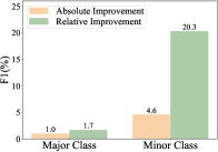
Therefore, we compare the performance of both majority class and minority class to our baseline model. Table 2(b) shows that, the minority class achieves a greater improvement of 4.6% F1 score and 20.3% relative improvement compared to baseline, while majority class only achieves 1.0% and 1.7% improvement respectively. The positive effect on the performance of minority class demonstrates the effectiveness of confusion relations, which can reasonably explain where the uncertainty of an event pair’s temporal relationship comes from. Besides, by providing more opportunities for our model to explore and learn the knowledge of minority classes, it enables us to better understand the minority class, and alleviates the imbalanced label distribution issue to some extent.
5.5 Utilizing Vague Efficiently

Event pairs with temporal relation Vague contain sufficient information about well-defined relations. In our approach, our model learns the meaning of a well-defined relation not only from itself, but also from Vague. The importance of supplementary information provided by Vague could be more obvious when the training resources are limited. Therefore, to evaluate our model’s capability in effectively exploring sufficient information from training data, we conduct experiments with variable amounts of training data, ranging from 5% to 50%, while keeping the test set unchanged. In low resources scenarios, our model outperforms baseline model by 7.1% on average F1 score. Figure 3 illustrates the experiment results of the F1 scores of baseline model and our model on TB-Dense.
We can observe that, our model stably outperforms baseline model in every portion of the training set. This result indicates that our model is more capable of capturing the information in Vague efficiently and making full use of it. When the smaller size of the training set is used, such as 5% to 30%, our model shows a larger difference from baseline. This phenomenon mainly results from the different amounts of information models can obtain. Since there are only a few well-defined relations in the small training set, single-label classification-based models are struggling to recognize them correctly. However, our model’s capability in leveraging Vague to learn knowledge of well-defined relations plays an important role, which helps to capture effective information from the limited training set more comprehensively and efficiently.
In addition, due to the imbalanced label distribution, minority classes like Include and Is included are hardly included in the small training set. Therefore, single-label classification-based methods may have difficulty in making predictions on these relations. Our method, on the other hand, can explore their information through a large amount of Vague, and achieves higher average F1 scores of 4.7% and 6.2% on Include and Is included respectively.
5.6 Interpretability of Vague
| Precision | Absolute Value | Relative Value | ||||
| Top1 | Top2 | Top3 | Top1 | Top2 | Top3 | |
| Random | 60.0 | 30.0 | 10.0 | 0.0 | 0.0 | 0.0 |
| Baseline | 76.9 | 48.7 | 19.9 | 28.2 | 62.3 | 99.0 |
| METRE | 82.1 | 63.1 | 28.2 | 36.8 | 110.3 | 182.0 |
| Improve. | +5.2 | +14.4 | + 8.3 | *1.30 | *1.77 | *1.84 |
Treated as a multi-label classification task, our model is able to predict relations composition of Vague. To better evaluate the prediction accuracy, we check the consistency between our prediction of Vague and the annotation results from humans. As we mentioned in Section 4.1, every event pair’s relation is determined by 3 annotators, so we can calculate the overlap of the prediction of our model with the 3 different annotation results. Specifically, if we make a correct prediction on Vague, we choose the Top relations and judge whether these relations all conform to the annotation results. The precision scores are shown in Table 6.
Our model outperforms baseline by 5.2%, 14.4% and 8.3% in Top1/2/3 precision respectively, demonstrating a greater capability of our model in predicting the intrinsic composition of Vague. Given the precision of random ranking, we calculate the relative precision value as and . As increases, our model shows a larger improvement in relative precision than baseline, from 1.30 times to 1.84 times, which indicates that our advantage is more obvious when the model is asked to provide full information of Vague.
6 Conclusion
In this work, we investigate the underlying meaning of the special relation Vague in the temporal relation extraction task. A novel approach is proposed to effectively utilize the latent connection between Vague and well-defined relations, helping our model understand the meaning of each relation more accurately. Experiments show that our model achieves better or comparable performance compared to previous state-of-the-art methods on three benchmarks, indicating the effectiveness of our approach. Extensive analyses further demonstrate our model’s advantage in using training data more comprehensively and making our predictions more interpretable.
Limitations
There are only 3 well-defined relations in MATRES and none of them have confusion relation, as these relations are only determined by the start-point relations. Thus the diversity of is constrained due to the absence of confusion relation and the small size of well-defined relations, which further influences its effectiveness in assisting the model’s understanding of Vague. Besides, there is not a proper confusion relation for Simultaneous currently. Therefore, we still need to figure out a better constitution of and further improve the performance of our model.
References
- Cassidy et al. (2014) Taylor Cassidy, Bill McDowell, Nathanael Chambers, and Steven Bethard. 2014. An annotation framework for dense event ordering. In Proceedings of the 52nd Annual Meeting of the Association for Computational Linguistics (Volume 2: Short Papers), pages 501–506.
- Cheng and Miyao (2017) Fei Cheng and Yusuke Miyao. 2017. Classifying temporal relations by bidirectional LSTM over dependency paths. In Proceedings of the 55th Annual Meeting of the Association for Computational Linguistics (Volume 2: Short Papers), pages 1–6, Vancouver, Canada. Association for Computational Linguistics.
- Coll-Florit and Gennari (2011) Marta Coll-Florit and Silvia P. Gennari. 2011. Time in language: Event duration in language comprehension. Cognitive Psychology, 62(1):41–79.
- Devlin et al. (2019) Jacob Devlin, Ming-Wei Chang, Kenton Lee, and Kristina Toutanova. 2019. BERT: Pre-training of deep bidirectional transformers for language understanding. In Proceedings of the 2019 Conference of the North American Chapter of the Association for Computational Linguistics: Human Language Technologies, Volume 1 (Long and Short Papers), pages 4171–4186, Minneapolis, Minnesota. Association for Computational Linguistics.
- Han et al. (2019) Rujun Han, Qiang Ning, and Nanyun Peng. 2019. Joint event and temporal relation extraction with shared representations and structured prediction. arXiv preprint arXiv:1909.05360.
- Hwang et al. (2022) EunJeong Hwang, Jay-Yoon Lee, Tianyi Yang, Dhruvesh Patel, Dongxu Zhang, and Andrew McCallum. 2022. Event-event relation extraction using probabilistic box embedding. In Proceedings of the 60th Annual Meeting of the Association for Computational Linguistics (Volume 2: Short Papers), pages 235–244, Dublin, Ireland. Association for Computational Linguistics.
- Liu et al. (2019) Yinhan Liu, Myle Ott, Naman Goyal, Jingfei Du, Mandar Joshi, Danqi Chen, Omer Levy, Mike Lewis, Luke Zettlemoyer, and Veselin Stoyanov. 2019. Roberta: A robustly optimized bert pretraining approach. arXiv preprint arXiv:1907.11692.
- Malinin and Gales (2018) Andrey Malinin and Mark Gales. 2018. Predictive uncertainty estimation via prior networks.
- Malinin and Gales (2019) Andrey Malinin and Mark Gales. 2019. Reverse kl-divergence training of prior networks: Improved uncertainty and adversarial robustness.
- Man et al. (2022) Hieu Man, Nghia Trung Ngo, Linh Ngo Van, and Thien Huu Nguyen. 2022. Selecting optimal context sentences for event-event relation extraction. Proceedings of the AAAI Conference on Artificial Intelligence, 36(10):11058–11066.
- Mathur et al. (2021) Puneet Mathur, Rajiv Jain, Franck Dernoncourt, Vlad Morariu, Quan Hung Tran, and Dinesh Manocha. 2021. TIMERS: Document-level temporal relation extraction. In Proceedings of the 59th Annual Meeting of the Association for Computational Linguistics and the 11th International Joint Conference on Natural Language Processing (Volume 2: Short Papers), pages 524–533, Online. Association for Computational Linguistics.
- Meng et al. (2017) Yuanliang Meng, Anna Rumshisky, and Alexey Romanov. 2017. Temporal information extraction for question answering using syntactic dependencies in an LSTM-based architecture. In Proceedings of the 2017 Conference on Empirical Methods in Natural Language Processing, pages 887–896, Copenhagen, Denmark. Association for Computational Linguistics.
- Ng et al. (2014) Jun-Ping Ng, Yan Chen, Min-Yen Kan, and Zhoujun Li. 2014. Exploiting timelines to enhance multi-document summarization. In Proceedings of the 52nd Annual Meeting of the Association for Computational Linguistics (Volume 1: Long Papers), pages 923–933, Baltimore, Maryland. Association for Computational Linguistics.
- Ning et al. (2018) Qiang Ning, Hao Wu, and Dan Roth. 2018. A multi-axis annotation scheme for event temporal relations. In Proceedings of the 56th Annual Meeting of the Association for Computational Linguistics (Volume 1: Long Papers), pages 1318–1328.
- Shi et al. (2019) Weiyan Shi, Tiancheng Zhao, and Zhou Yu. 2019. Unsupervised dialog structure learning. In Proceedings of the 2019 Conference of the North American Chapter of the Association for Computational Linguistics: Human Language Technologies, Volume 1 (Long and Short Papers), pages 1797–1807, Minneapolis, Minnesota. Association for Computational Linguistics.
- Styler IV et al. (2014) William F. Styler IV, Steven Bethard, Sean Finan, Martha Palmer, Sameer Pradhan, Piet C de Groen, Brad Erickson, Timothy Miller, Chen Lin, Guergana Savova, and James Pustejovsky. 2014. Temporal annotation in the clinical domain. Transactions of the Association for Computational Linguistics, 2:143–154.
- UzZaman et al. (2013) Naushad UzZaman, Hector Llorens, Leon Derczynski, James Allen, Marc Verhagen, and James Pustejovsky. 2013. Semeval-2013 task 1: Tempeval-3: Evaluating time expressions, events, and temporal relations. In Second Joint Conference on Lexical and Computational Semantics (* SEM), Volume 2: Proceedings of the Seventh International Workshop on Semantic Evaluation (SemEval 2013), pages 1–9.
- Vashishtha et al. (2019) Siddharth Vashishtha, Benjamin Van Durme, and Aaron Steven White. 2019. Fine-grained temporal relation extraction. In Proceedings of the 57th Annual Meeting of the Association for Computational Linguistics, pages 2906–2919, Florence, Italy. Association for Computational Linguistics.
- Verhagen et al. (2007) Marc Verhagen, Robert Gaizauskas, Frank Schilder, Mark Hepple, Graham Katz, and James Pustejovsky. 2007. Semeval-2007 task 15: Tempeval temporal relation identification. In Proceedings of the fourth international workshop on semantic evaluations (SemEval-2007), pages 75–80.
- Wadden et al. (2019) David Wadden, Ulme Wennberg, Yi Luan, and Hannaneh Hajishirzi. 2019. Entity, relation, and event extraction with contextualized span representations. In Proceedings of the 2019 Conference on Empirical Methods in Natural Language Processing and the 9th International Joint Conference on Natural Language Processing, EMNLP-IJCNLP 2019, Hong Kong, China, November 3-7, 2019, pages 5783–5788. Association for Computational Linguistics.
- Wang et al. (2020) Haoyu Wang, Muhao Chen, Hongming Zhang, and Dan Roth. 2020. Joint constrained learning for event-event relation extraction. arXiv preprint arXiv:2010.06727.
- Wang et al. (2022a) Haoyu Wang, Hongming Zhang, Yuqian Deng, Jacob R Gardner, Muhao Chen, and Dan Roth. 2022a. Extracting or guessing? improving faithfulness of event temporal relation extraction. arXiv preprint arXiv:2210.04992.
- Wang et al. (2022b) Xiaozhi Wang, Yulin Chen, Ning Ding, Hao Peng, Zimu Wang, Yankai Lin, Xu Han, Lei Hou, Juanzi Li, Zhiyuan Liu, et al. 2022b. Maven-ere: A unified large-scale dataset for event coreference, temporal, causal, and subevent relation extraction. arXiv preprint arXiv:2211.07342.
- Wen and Ji (2021) Haoyang Wen and Heng Ji. 2021. Utilizing relative event time to enhance event-event temporal relation extraction. In Proceedings of the 2021 Conference on Empirical Methods in Natural Language Processing, pages 10431–10437, Online and Punta Cana, Dominican Republic. Association for Computational Linguistics.
- Yu et al. (2017) Mo Yu, Wenpeng Yin, Kazi Saidul Hasan, Cicero dos Santos, Bing Xiang, and Bowen Zhou. 2017. Improved neural relation detection for knowledge base question answering. In Proceedings of the 55th Annual Meeting of the Association for Computational Linguistics (Volume 1: Long Papers), pages 571–581, Vancouver, Canada. Association for Computational Linguistics.
- Zhang et al. (2022) Shuaicheng Zhang, Qiang Ning, and Lifu Huang. 2022. Extracting temporal event relation with syntactic-guided temporal graph transformer. Proceedings of the 2022 Conference of the North American Chapter of the Association for Computational Linguistics: Human Language Technologies, NAACL-HLT 2022,.
- Zhong and Chen (2021) Zexuan Zhong and Danqi Chen. 2021. A frustratingly easy approach for entity and relation extraction. In Proceedings of the 2021 Conference of the North American Chapter of the Association for Computational Linguistics: Human Language Technologies, pages 50–61.
- Zhou et al. (2020) Wenxuan Zhou, Kevin Huang, Tengyu Ma, and Jing Huang. 2020. Document-level relation extraction with adaptive thresholding and localized context pooling.
Appendix A Dataset Statistics
| Dataset | TB-Dense | MATRES | UDS-T |
| Before | 808 | 5483 | 2427 |
| After | 674 | 3651 | 323 |
| Include | 206 | - | 523 |
| Is included | 273 | - | 514 |
| Simultaneous | 59 | 376 | 86 |
| Vague | 2012 | 1320 | 1217 |
| Vague Proportion | 49.9% | 12.2% | 23.9% |
| Dataset | TB-Dense | MATRES | UDS-T |
| Before | 1348 | 6853 | 3316 |
| After | 1120 | 4548 | 439 |
| Include | 276 | - | 784 |
| Is included | 347 | - | 693 |
| Simultaneous | 93 | 470 | 119 |
| Vague | 2012 | 1631 | 1682 |
| Vague Proportion | 47.7% | 12.1% | 23.9% |
Appendix B UDS-T Mapping Rules
| start-point | end-point | relation |
| before | before | Before |
| before | equal | Include |
| before | after | Include |
| equal | before | Is included |
| equal | equal | Simultaneous |
| equal | after | Include |
| after | before | Is included |
| after | equal | Is included |
| after | after | After |
In UDS-T, instead of determining the temporal relation between an event pair explicitly, annotators are required to determine the relative timeline between every event pair. There are only three temporal relations between a time-point pair: before, after and equal, and we can deduce the temporal relation according to the relation definition in TB-Dense, as shown in Table 9.
Every event pair in the training set of UDS-T is annotated by only one person, where inconsistency and ambiguity will not happen and Vague is not considered in the training set. The validation set and test set, on the other hand, are annotated by three different people per event pair. Therefore, we use majority voting to decide which temporal relation of an event pair should be. Specifically, if two or three people make the same decision, we hold it as the temporal relation between this event pair, while if three annotators make totally different decisions, we view it as Vague, and take all these three decisions as the possible relations between this event pair. Since only the validation set and test set of UDS-T contain Vague, we split them into the new training/validation/test set to fit the temporal relation task in our work, with the proportion of 80%/10%/10% respectively.