Online Tensor-Based Learning for Multi-Way Data
Abstract.
The online analysis of multi-way data stored in a tensor has become an essential tool for capturing the underlying structures and extracting the sensitive features which can be used to learn a predictive model. However, data distributions often evolve with time and a current predictive model may not be sufficiently representative in the future. Therefore, incrementally updating the tensor-based features and model coefficients are required in such situations. A new efficient tensor-based feature extraction, named NeSGD, is proposed for online (CP) decomposition. According to the new features obtained from the resultant matrices of NeSGD, a new criteria is triggered for the updated process of the online predictive model. Experimental evaluation in the field of structural health monitoring using laboratory-based and real-life structural datasets show that our methods provide more accurate results compared with existing online tensor analysis and model learning. The results showed that the proposed methods significantly improved the classification error rates, were able to assimilate the changes in the positive data distribution over time, and maintained a high predictive accuracy in all case studies.
1. Introduction
Almost all major cities around the world have developed complex physical infrastructure that encompasses bridges, towers, and iconic buildings. One of the most emerging challenges with such infrastructure is to continuously monitor its health to ensure the highest levels of safety. Most of the existing structural monitoring and maintenance approaches rely on a time-based visual inspection and manual instrumentation methods which are neither efficient nor effective.
Internet of Things (IoT) has created a new paradigm for connecting things (e.g., computing devices, sensors and objects) and enabling data collection over the Internet. Nowadays, various types of IoT devices are widely used in smart cities to continuously collect data that can be used to manage resources efficiently. For example, many sensors are connected to bridges to collect various types of data about their health status. This data can be then used to monitor the health of the bridges and decide when maintenance should be carried out in case of potential damage (Li et al., 2015). With this advancement, the concept of smart infrastructure maintenance has emerged as a continuous automated process known as Structural Health Monitoring (SHM) (Ou and Li, 2010).
SHM provides an economic monitoring approach as the inspection process which is mainly based on a low-cost IoT data collection system. It also improves effectiveness due to the automation and continuity of the monitoring process. SHM enhances understanding the behaviour of structures as it continuously provides large data that can be utilized to gain insight into the health of a structure and make timely and economic decisions about its maintenance.
One of the critical challenges in SHM is the non-stationary nature of the data collected from several networked sensors attached to a bridge (Xin et al., 2018). This collected data is the foundation for training a model to detect potential damages in a bridge. In SHM, the data used in training the model comes from healthy samples (it does not include damaged data set) and hence represents one-class data. Also, the data is collected within a fixed period time and processed simultaneously. This influences the performance of model training as it does not consider data variations over more extended period time. Structures always experience severe events such as heavy loads over a long and continuous period of time and high and low seasonal temperatures. Such variations would dramatically affect the status of the data as it changes the characteristics of the structure such as the data frequencies. Consequently, the training data fed into the model does not represent such variations but only healthy or undamaged data samples. Thus it is critical to develop a method that mitigates these variations and increases the specificity rate.
Another challenge in SHM is that generated sensing data exists in a correlated multi-way form which makes the standard two-way matrix analysis unable to capture all of these correlations and relationships (Cheema et al., 2016). Instead, the SHM data can be arranged into a three-way data structure where each data point is triple of a feature value extracted from a particular sensor at a specific time. Here, the information extracted from the raw signals in time domain represent features, the sensors represent data location and time snapshots represent the timestamps when data was extracted (as shown in Figure 1).

In order to address the problem as mentioned above, an online one-class learning approach should be employed along with an online multi-way data analysis tool to capture the underlying structure inherits in multi-way sensing data. In this setting, the design of a one-class support vector machine (OCSVM) (Anaissi et al., 2017a) and tensor analysis are well-suited to this kind of problems where only observations from the multi-way positive (healthy) samples are required.
Tensor is a multi-way extension of the matrix to represent multidimensional data structures such that SHM data. Tensor analysis requires extensions to the traditional two-way data analysis methods such as Non-negative Matrix Factorization (NMF), Principal Component Analysis (PCA) and Singular Value Decomposition (SVD). In this sense, the CANDECOMP/PARAFAC (CP) (Phan et al., 2013) has recently become a standard approach for analyzing multi-way tensor data. Several algorithms have been proposed to solve CP decomposition (Symeonidis et al., 2008) (Lebedev et al., 2014) (Rendle et al., 2009). Among these algorithms, alternating least square(ALS) has been heavily employed which repeatedly solves each component matrix by locking all other components until it converges (Papalexakis et al., 2017). It is usually applied in offline mode to decompose the positive training tensor data, which then fed into an OCSVM model to construct the decision boundary. However, this offline process is also not suitable for such dynamically changing SHM data. Therefore, we also interested here to incrementally update the resultant CP decomposition in an online manner.
Similarly, the OCSVM has become a standard approach in solving anomaly detection problems. OCSVM is usually trained with a set of positive (healthy) training data, which are collected within a fixed time period and are processed together at once. As we mentioned before, this fixed batch model generally performs poorly if the distribution of the training data varies over a time span. One simple approach would be to retrain the OCSVM model from scratch when additional positive data arrive. However, this would lead to ever-increasing training sets, and would eventually become impractical. Moreover, it also seems computationally wasteful to retrain the model for each incoming datum, which will likely have a minimal effect on the previous decision boundary. Another approach for dealing with large non-stationary data would be to develop an online-OCSVM model that incrementally updates the decision boundary, i.e., incorporating additional healthy data when they are available without retraining the model from scratch. The question now is how to distinguish real damage from the environmental changes which require model updates. Current research (such as (Wang et al., 2013; Davy et al., 2006)) proposes a threshold value to measure the closeness of a new negative datum to the decision boundary for online OCSVM. More specifically, if this new negative datum is not far from the decision boundary, then they consider it as a healthy sample (environmental changes) and update the model accordingly. However, this predefined threshold is very sensitive to the distribution of the training data and it may include or exclude anomalies and healthy samples. Recently, Anaissi et al.(Anaissi et al., 2017b) propose another approach which measures the similarity between a new event and error support vectors to generate a self-advised decision value rather than using a fixed threshold. That was an effective solution but it is susceptible to include damage samples if the model keeps updated in the same direction as the real damage samples. Then the resultant updated model will start encounter damage samples in the training data. Thus this approach will start missing real damage events.
To address the aforementioned problems, we propose a new method that uses the online learning technique to solve the problems of online OCSVM and CP decomposition. We employ stochastic gradient descent (SGD) algorithm for online CP decompositio, and we introduce a new criterion to trigger the update process of the online-OCSVM, This criterion utilities the information derived from the location component matrix which we obtain when we decompose the three-way tensor data . This matrix stores meaningful information about the behavior for each sensor location on the bridge. Intuitively, environmental changes such as temperature will affect all the instrumented sensors on the bridge similarly. However, real damage would affect a particular sensor location and the ones close by. The contributions of our proposed method are as follows:
-
•
Online CP decomposition. We employ Nesterov’s Accelerated Gradient (NAG) method into SGD algorithm to solve the CP decomposition which has the capability to update in one single step. We also followed the perturbation approach which adds a little noise to the gradient update step to reinforce the next update step to start moving away from a saddle point toward the correct direction.
-
•
Online anomaly detection. We propose a tensor-based online-OCSVM which is able to distinguish between environmental and damage behaviours to adequately update the model coefficients.
-
•
Empirical analysis on structural datasets. We conduct experimental analysis using laboratory-based and real-life datasets in the field of SHM. The experimental analysis shows that our method can achieve lower false alarm rates compared to other known existing online and offline methods.
This paper is organized as follows. Section 2 presents preliminary work and discusses research related to this work. In section 3 we introduce the details of our method; online OCSVM-OCPD. Section 4 presents the experimental evaluation of the proposed method and discuses the results. Conclusions and future work are discussed in Section 5.
2. Preliminaries and Related Work
Our research work builds upon and extends essential methods and algorithms including Tensor (CP) Decomposition, Stochastic Gradient Descent, and Online One-Class Support Vector Machine. We first discuss the key elements of these methods and algorithms and then follow that with an analysis of related studies and their contribution to addressing the challenges discussed in the introduction. We conclude this with the discussion with the weaknesses of existing work and how our proposed work attempts to address these weaknesses.
2.1. CP Decomposition
Given a three-way tensor , CP decomposes into three matrices , and , where is the latent factors. It can be written as follows:
| (1) |
where ”” is a vector outer product. is the latent element, and are r-th columns of component matrices , and . The main goal of CP decomposition is to decrease the sum square error between the model and a given tensor . Equation 2 shows our loss function needs to be optimized.
| (2) |
where is the sum squares of and the subscript is the Frobenius norm. The loss function presented in Equation 2 is a non-convex problem with many local minima since it aims to optimize the sum squares of three matrices. The CP decomposition often uses the Alternating Least Squares (ALS) method to find the solution for a given tensor. The ALS method follows the offline training process which iteratively solves each component matrix by fixing all the other components, then it repeats the procedure until it converges (Khoa et al., 2017). The rational idea of the least square algorithm is to set the partial derivative of the loss function to zero concerning the parameter we need to minimize. Algorithm 1 presents the detailed steps of ALS.
-
1:
Initialize
-
2:
Repeat
-
3:
-
4:
-
5:
-
( is the unfolded matrix of in a current mode)
-
6:
until convergence
In online settings, it is a naive approach would be to recompute the CP decomposition from scratch for each new incoming . Therefore, this would become impractical and computationally expensive as new incoming datum would have a minimal effect on the current tensor. Zhou et al. (Zhou et al., 2016) proposed a method called onlineCP to address the problem of online CP decomposition using the ALS algorithm. The method was able to incrementally update the temporal mode in multi-way data but failed for non-temporal modes (Khoa et al., 2017). In recent years, several studies have been proposed to solve the CP decomposition using the stochastic gradient descent (SGD) algorithm which will be discussed in the following section.
2.2. Stochastic Gradient Descent
Stochastic gradient descent algorithm is a key tool for optimization problems. Assume that our aim is to optimize a loss function , where is a data point drawn from a distribution and is a variable. The stochastic optimization problem can be defined as follows:
| (3) |
The stochastic gradient descent method solves the above problem defined in Equation 13 by repeatedly updates to minimize . It starts with some initial value of and then repeatedly performs the update as follows:
| (4) |
where is the learning rate and is a random sample drawn from the given distribution .
This method guarantees the convergence of the loss function to the global minimum when it is convex. However, it can be susceptible to many local minima and saddle points when the loss function exists in a non-convex setting. Thus it becomes an NP-hard problem. The main bottleneck here is due to the existence of many saddle points and not to the local minima (Ge et al., 2015). This is because the rational idea of gradient algorithm depends only on the gradient information which may have even though it is not at a minimum.
Recently, SGD has attracted several researchers working on tensor decomposition. For instance, Ge et al.(Ge et al., 2015) proposed a perturbed SGD (PSGD) algorithm for orthogonal tensor optimization. They presented several theoretical analysis that ensures convergence; however, the method does not apply to non-orthogonal tensor. They also didn’t address the problem of slow convergence. Similarly, Maehara et al.(Maehara et al., 2016) propose a new algorithm for CP decomposition based on a combination of SGD and ALS methods (SALS). The authors claimed the algorithm works well in terms of accuracy. Yet its theoretical properties have not been completely proven and the saddle point problem was not addressed. Rendle and Thieme (Rendle and Schmidt-Thieme, 2010) propose a pairwise interaction tensor factorization method based on Bayesian personalized rank. The algorithm was designed to work only on three-way tensor data. To the best of our knowledge, this is the first work that applies SGD algorithm augmented with Nesterov’s optimal gradient and perturbation methods for optimal CP decomposition of multi-way tensor data.
2.3. Online One-Class Support Vector Machine
Given a set of training data , with being the number of samples, OCSVM maps these samples into a high dimensional feature space using a function through the kernel . Then OCSVM learns a decision boundary that maximally separates the training samples from the origin (Schölkopf et al., 2001). The primary objective of OCSVM is to optimize the following equation:
| (5) |
where is a user defined parameter to control the rate of anomalies in the training data, are the slack variable, is the kernel matrix and is the separating hyperplane in the feature space. The problem turns into a dual objective by introducing Lagrange multipliers . This dual optimization problem is solved using the following quadratic programming formula (Schölkopf and Smola, 2002):
| (6) |
where is the kernel matrix, are the Lagrange multipliers and known as the bias term.
The partial derivative of the quadratic optimization problem (defined in Equation 6) with respect to , , is then used as a decision function to calculate the score for a new incoming sample:
| (7) |
The OCSVM uses Equation 8 to identify whether a new incoming point belongs to the positive class when returning a positive value, and vice versa if it generates a negative value.
| (8) |
The achieved OCSVM solution must always satisfy the constraints from the Karush-Khun-Tucker (KKT) conditions, which are described in Equation 12.
| (12) |
where is referred to the non-support or reserve training vectors denoted by R, represents non-margin support or error vectors denoted by E and represents the support vectors denoted by S.
In an online setting, we need to ensure the KKT conditions are maintained while learning and adding a new data point to the previous solution. Several researchers address the problem of online SVM (Cauwenberghs and Poggio, 2000; Diehl and Cauwenberghs, 2003; Laskov et al., 2006) where all are based on the original method known as bookkeeping which proposed by Cauwenberghs et al.. The method computes the new coefficients of the SVM model while preserving the KKT conditions. This method made useful contributions to the incremental learning of two classes SVM (TCSVM), but it cannot be used for the one-class problem. Davy et al. (Davy et al., 2006) concluded that such incremental SVM methods cannot be directly applied to the one-class problem as they are dependent on the TCSVM margin areas which do not exist in OCSVM. Therefore, Davy et al.proposed an online OCSVM-based threshold value. In this method, the anomaly score is computed for each incoming datum and evaluated against a predefined threshold value. The new datum is added to the training data and the model coefficients are updated accordingly when its value is greater than the threshold. Similarly, Wang et al.(Wang et al., 2013) presented an online OCSVM algorithm for detecting abnormal events in real-time video surveillance. Their algorithm combines online least-squares OCSVM (LS-OCSVM) and sparse online LS-OCSVM. The basic model is initially constructed through a learning training set with a limited number of samples. Like (Davy et al., 2006) algorithm, the model is then updated through each incoming datum using threshold-based evaluation. Recently, Anaissi et al. (Anaissi et al., 2017b) propose another approach which measures the similarity between a new event and error support vectors to generate a self-advised decision value rather than using a fixed threshold. That was an effective solution but it is susceptible to include damage samples if the model keeps updated in the same direction as the real damage samples. Then the resultant updated model will start encountering damage samples in the training data. Thus this approach will start missing the real damage events.
3. Online Tensor-Based Learning for Multi-Way Data
The incremental learning of online-OCSVM has been well-studied and proved to produce the same solution as the batch learning process (offline learning). In fact, the main problem of online-OCSVM is not related to the incremental learning process, but it is due to the criteria we need to trigger this update process successfully. Given an OCSVM model constructed from the healthy training data, the calculated decision value using Equation 7 will decide whether a new event is healthy or not. When this decision value is positive i.e., healthy, then the KKT conditions remain satisfied when this new datum is added to the training data. Thus no model update is required. On the other hand, when this decision value is negative, we need to know whether this event is related to damage data or it is only due to environmental changes such as temperature. If this event is real damage then we report it without any model update. Nevertheless, if it is due to environmental changes, we need to add this datum to the training data and update the model coefficients accordingly since this negative decision datum will violate the KKT conditions. The challenge now is how to separate the environmental changes from real damage.
In this paper, we propose a new criterion to trigger the update process of the online-OCSVM based on the information derived from the location component matrix, we obtain when we decompose the three-way tensor data . This matrix stores meaningful information about the behavior for each sensor location on the bridge. Intuitively, environmental changes such as temperature will affect all the instrumented sensors on the bridge similarly. However, real damage would affect a particular sensor location and the ones close by. To implement this approach, we need to find an efficient solution for online-CP decomposition which will be discussed in the following section.
3.1. Nesterov SGD (NeSGD) for Online-CP Decomposition
We employ stochastic gradient descent (SGD) algorithm to perform CP decomposition in online manner. SGD has the capability to deal with big data and online learning models. The key element for optimization problems in SGD is defined as:
| (13) |
where is the loss function needs to be optimized, is a data point and is a variable.
The SGD method solves the above problem defined in Equation 13 by repeatedly updates to minimize . It starts with some initial value of and then repeatedly performs the update as follows:
| (14) |
where is the learning rate and is the partial derivative of the loss function with respect to the parameter we need to minimize i.e. .
In the setting of tensor decomposition, we need to calculate the partial derivative of the loss function defined in Equation 2 with respect to the three modes and alternatively as follows:
| (15) | |||
where is an unfolding matrix of tensor in mode . The gradient update step for and are as follows:
| (16) | |||
The rational idea of GSD algorithm depends only on the gradient information of . In such a non-convex setting, this partial derivative may encounter data points with even though it is not at a global minimum. These data points are known as saddle points which may detente the optimization process to reach the desired local minimum if not escaped (Ge et al., 2015). These saddle points can be identified by studying the second-order derivative (aka Hessian) . Theoretically, when the , must be a local minimum; if , then we are at a local maximum; if has both positive and negative eigenvalues, the point is a saddle point. The second order-methods guarantee convergence, but the computing of Hessian matrix is high, which makes the method infeasible for high dimensional data and online learning. Ge et al.(Ge et al., 2015) show that saddle points are very unstable and can be escaped if we slightly perturb them with some noise. Based on this, we use the perturbation approach which adds Gaussian noise to the gradient. This reinforces the next update step to start moving away from that saddle point toward the correct direction. After a random perturbation, it is highly unlikely that the point remains in the same band and hence it can be efficiently escaped (i.e., no longer a saddle point)(Jin et al., 2017). Since we are interested in the fast optimization process due to online settings, we further incorporate Nesterov’s method into the PSGD algorithm to accelerate the convergence rate. Recently, Nesterov’s Accelerated Gradient (NAG) (Nesterov, 2013) has received much attention for solving convex optimization problems (Guan et al., 2012; Nitanda, 2014; Ghadimi and Lan, 2016). It introduces a smart variation of momentum that works slightly better than standard momentum. This technique modifies the traditional SGD by introducing velocity and friction , which tries to control the velocity and prevents overshooting the valley while allowing faster descent. Our idea behind Nesterov’s is to calculate the gradient at a next position that we know our momentum will reach it instead of calculating the gradient at the current position. In practice, it performs a simple step of gradient descent to go from to , and then it shifts slightly further than in the direction given by . In this setting, we model the gradient update step with NAG as follows:
| (17) |
where
| (18) |
where is a Gaussian noise, is the step size, and are the regularization and penalization parameter into the norms to achieve smooth representations of the outcome and thus bypassing the perturbation surrounding the local minimum problem. The updates for and are similar to the aforementioned ones. With NAG, our method achieves a global convergence rate of comparing to for traditional gradient descent. Based on the above models, we present our NeSGD algorithm 2.
3.2. Tensor-based Advised Decision Values
In this paper, we introduce a new criterion to trigger the update process when the online OCSVM model generates a negative decision value for a new sample . Based on the information derived from the location component matrix which we obtain when we decompose a three-way tensor data , we generate an advised decision score for a new negative datum based on the average distance from a sensing location matrix (a row in (B)) to the k nearest neighbouring (knn) locations. A big change in this score of a sensing location indicates a change in sensor behaviour which might be due to occurred damage or environmental changes. If all the knn scores behave differently, then this indicates that the negative decision value is due to environmental changes. Therefore, we add this new datum to the training data and update the model coefficients accordingly. Otherwise, we report as an anomaly data point. This algorithm is described as follows: given the location matrix , the unit vector of each point with its closest points is computed as follows:
| (19) |
Then we estimate the change occurred in sensors behaviors based on the absolute difference between and using the following equation
| (20) |
where represents the probability of that negative decision value of is being related to environmental changes, and is a small value represents acceptable change. In this work, we set-up a 90% confidence interval for to judge whether a new datum belongs to the healthy sample or not. In fact, this confidence interval is based on the physical layout of the sensor instrumentation. Algorithm 3 illustrates the process of generating the tensor-based advised decision values:
3.3. Model Coefficients Update
The model solution of OCSVM is basically composed of two coefficients denoted by and . When a new datum arrives with an advised decision value , the model coefficients must be updated to get the new solution and , which should preserve the KKT conditions (see Equation 12). We initially assign a zero value to and then start looking for the largest possible increment of until its becomes zero, in this case is added to the support vectors set . If equals to , is added to the set of the error vectors .
The difference between the two states of OCSVM is shown in the following equation:
| (21) |
Since , we can write Equation 21 in a matrix form as follows:
| (28) |
| (29) |
The goal now is to determine the index of the sample that leads to the minimum . As in (Cauwenberghs and Poggio, 2000), five cases must be considered to manage the migration of the sample between the three sets , and , and calculate .
-
(1)
, and .
leads to the minimum Move from to . -
(2)
, and
leads to the minimum Move from to . -
(3)
= , and or and .
leads to the minimum Move from or to . -
(4)
, is the index of .
leads to the minimum Move to , terminate. -
(5)
, is the index of .
leads to the minimum Move to , terminate.
The next step after the migration is to update the inverse matrix . Two cases to consider during the update: extending when the determined index joins , or compressing when index leaves . Similar to (Laskov et al., 2006), we applied the Sherman-Morrison-Woodbury formula to obtain the new matrix . We repeat this procedure until the index is related to the new example .
4. Experimental Results
We conduct all our experiments using an Intel(R) Core(TM) i7 CPU 3.60GHz with 16GB memory. We use R software to implement our algorithms with the help of the two packages; the rTensor and the e1071 for tensor tools and one-class model.
4.1. Experiments on Synthetic Data
4.1.1. NeSGD convergence
Our initial experiment was to ensure the convergence of our NeSGD algorithm and compare it to other state-of-the-art methods such as SGD, PSGD, and SALS algorithms in terms of robustness and convergence. We generated a synthetic long time dimension tensor from 12 random loading matrices in which entries were drawn from uniform distribution . We evaluated the performance of each method by plotting the number of samples versus the root mean square error (RMSE). For all experiments we use the learning rate . It can be clearly seen from Figure 2 that NeSGD outperformed the SGD and PSGD algorithms in terms of convergence and robustness. Both SALS and NeCPD converged to a small RMSE but it was lower and faster in NeSGD.

4.1.2. Tensor-based analysis
The same synthetic data is used here but with some modifications to evaluate the performance of the proposed method of tensor-based advice decision value. We initially emulate environmental changes on the last 300 samples by modifying the random generator setting , where is the mean and is the standard deviation, in all since environmental changes which will naturally affect all sensors, where each matrix in represents one source (i.e location). The first 700 samples were generated under the same environmental conditions in which 500 samples are used to form the training tensor . The NeSGD is initially applied to decompose the tensor into three matrices and given , and the matrix is then used to learn the OCSVM. The remaining 200 samples where fed sequentially to the online NeSGD and OCSVM in addition to the environmental affected 300 samples. For each incoming datum, we compute and which is presented to the online OCSVM algorithm to calculate its health score. If that datum is predicted as healthy then the model is not updated. However, if that datum is predicted as unhealthy, then we compute the tensor-based decision value using Equation 20. If its advice decision value is greater than then we incorporated this new datum into the training data and we updated the model’s coefficients accordingly. Figure 3 shows the initial 500 training samples where the blue dots represent the resultant support vectors of the offline model. Figure 5 shows the resultant decision boundary after we incrementally updated the OCSVM model. As it can be seen, all the healthy samples were successfully incorporated into the model since these samples were slightly different from the training samples due to the environmental changes. We can also observe that the KNN score for all sensor were significantly increased which indicates the negative decision values were due to environmental changes. Further, it shows how the decision boundary grew over time and incorporated new healthy samples.


4.2. Case Studies in Structural Health Monitoring
To further validate our model, we evaluate the performance of our Tensor-based advice decision values for incremental OCSVM when it is applied to SHM. The evaluation is based on real SHM data collected from two case studies namely (a) the Infante D. Henrique Bridge in Portugal and (b) AusBridge a major Bridge in Australia (the actual Bridge name cannot be published due to a data confidentiality agreement).
4.2.1. Infante D. Henrique Bridge Data
The SHM data is collected continuously from the Infante D. Henrique Bridge bridge (shown in Figure 5 (a)) over a period of two years (from September 2007 to September 2009) (Comanducci et al., 2016; Magalhães et al., 2012). The data collection was carried out continuously by instrumenting the bridge with 12 force-balance highly sensitive accelerometers to measure acceleration. Every 30 minutes, the collected acceleration measurements were retrieved from these sensors and input into an operational modal analysis process to determine the natural frequencies (the model parameters) of the bridge. This process resulted in 120 natural frequencies which used as the characteristic features in our study. Thus, this dataset consists of (35,040) samples each with 24 features. The resultant matrices from the 12 sensors were fused in a tensor . Besides acceleration measurements, temperatures were also recorded every 30 minutes because natural frequencies of the bridge can be influenced by environmental conditions (Comanducci et al., 2016; Magalhães et al., 2012).
Using this dataset, we run two-phase experimental analysis; In the first phase, we used the first two months of this data (i.e., 2,230 samples September-October 2007) to fuse them in a tensor which was decomposed using NeSGD method (see Algorithm 2) into three matrices , , and . The matrix is then used to construct an offline OCSVM model. We used the remaining 35,040 data samples to evaluate the offline OCSVM model without applying the tensor-based advice decision value method. This analysis resulted in a very high false alarm rate of 44.8%. This result demonstrates the significant effect of environmental factors, particularly the temperature, on the natural frequencies of the data collected from the bridge. In the second phase of this experiment, we run our proposed tensor-based advised incremental OCSVM algorithm on the same test dataset. Here, we calculated the health score for each incoming sample using equation 7. The algorithm then continues if the sample has been correctly classified, otherwise the tensor-based advice decision value has to be calculated to determine whether the model coefficients will have to be updated or not based on Equation 20.
The results of these experiments are shown in figure 5 (b); mainly resulted in a false alarm rate per month for the (tensor-based, threshold-based, self-advised) online OCSVM and the offline OCSVM. This figure also shows the monthly average temperature for the period of September 2007 and October 2007, which was used for constructing the offline OCSVM, for demonstrating the environmental conditions of the constructed model. As depicted in this figure, although the false alarm rate of our tensor-based online incremental model was high at the start of the experiment, it had decreased gradually until it reached close to zero as new arriving data augmented into the model.
By experimenting with the dataset during the period June 2008 - December 2008, our tensor-based online model recorded an above 10% false alarm rate. This period time belongs to the extreme temperature conditions which have not been previously experienced at that time point in the dataset. The self-advised method produces comparable results to tensor-based ones but with lower accuracy. In contrast to this, the threshold-based online OCSVM and offline OCSVM showed continuous some fluctuation in the false alarm rates in correlation with the monthly record temperature. Specifically, our tensor-based online model generated a very low false alarm rate (close to 0%) during the months which had temperature values that are significantly different from the temperature values recorded during the training period (i.e., September - October 2007 vs. September - October 2008). On the other hand, very high false alarm rates (close to 100%) were generated by the offline OCSVM model during the same time period.
From this case study, we conclude that environmental changes, which are captured using natural frequencies feature, can significantly influence OCSVM models. Our experiments with the real Infante D. Henrique Bridge dataset have demonstrated that our tensor-based online model is able to catch such environmental changes in the features. In this regard, the proposed method makes more accurate updated to the learning models compared to the (self-advised and threshold-based) online and offline models.


4.2.2. The AusBridge
In this case study, we collect acceleration data from the AusBridge using tri-axial accelerometers connected to a small computer under each jack arch. Every vehicle passed over a given jack arch it triggers an event on it. The sensors attached to that jack arch collected all the resulted vibrations for a duration of 1.6 seconds with a sampling rate of 375 Hz. As a result, each sensor captures 600 samples per event. The collected samples were further normalized and transformed into 300 features in the frequency domain.

We conducted two sets of experiments. The first one used a data of a total of 22,526 samples collected from 11 jack arches (nodes) during October 2015 and November 2016111The data for February 2016 had known instrumentation problem which appeared and was fixed during that period, and thus it was excluded from this experiment.. The data from the 11 nodes were fused in a tensor . We train the offline OCSVM model using the data collected in October 2015 (i.e ). The remaining data of (November 2015 - November 2016) was sequentially fed to the same model. Using the same dataset, we run these experiments with (self-advised and threshold-based) online OCSVM, offline OCSVM , and our tensor-based OCSVM model.
The false alarm error rates resulted from the experiments with the four OCSVM models are illustrated in Figure 6(a). The values are shown as averages over the 11 nodes for each month of the collected data. As shown, the offline OCSVM model generated an average of about 10% false alarm rate which means it classified many events as structural damage. Furthermore, the false alarm rates fluctuated with high standard deviations during most of the experiment period. This is not accurate and can lead to inappropriate decisions as all of the nodes being evaluated had no damage during the study period. Unlike the offline OCSVM model, our tensor-based online model resulted in a much lower false alarm rate, average about 0.1% with narrow standard deviations. The poor performance of the offline OCSVM model can be due to the environmental and operational conditions, which were not captured in the initial frequency features in the one-month training data (October 2016). The influence of these variations on the frequency features had been captured by the threshold-based online OCSVM method and enhanced its false alarm rates. As shown in the fugue, our tensor-based online OCSVM model resulted in lower false alarm rates compared to the other online models. Although setting a fixed threshold for a single OCSVM might be an easy task, but this is not practical. Such bridges comprised of 100’s of jack arches each of which is linked with an OCSVM model. Thus, setting a fixed threshold would require manual tuning of 100’s OCSVM models.
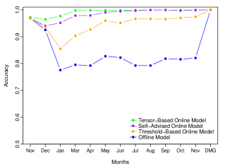
The goal of the second experiment set of the AusBridge case study was to confirm that even after a long-running period (i.e. 1 year) the updated model from our online OCSVM method still had the ability to detect structural damage. In the second experiment set of the AusBridge case study, we used the data of an identified damaged jack arch (node). In particular, we used 12 months of data during which the jack arch was health and 3 months of data while it was damaged. Our goal in this experiment is to confirm the reliability of our model in terms of its ability to detect structural damages even after a long time period (1 year). Using the 12 months dataset, we run the offline, self-advised, threshold-based, and our proposed tensor-based online OCSVM models. Figure 6 (b) shows the resulting accuracy of the four models over the 12-months of healthy data and the 3-months damaged data of the jack arch. As shown, the damage events were detected successfully by all the four models. In addition, our tensor-based model significantly outperformed the offline OCSVM and threshold-based incremental models by achieving lower false alarm rates.
5. Conclusion
We address the problem of learning from data sensed from networked sensors in IoT environments. Such data exists in a correlated multi-way form and considered as non-stationary due to the on-going variation that often arises from environmental changes over a long period time. Existing learning models such as OCSVM and traditional matrix analysis methods do not capture theses aspects. Thus, accuracy and performance are significantly affected with such non-stationary nature. We addressed these problems by proposing a new online CP decomposition named NeSGD and a Tensor-based Online-OCSVM method which employs the online learning technique. The essence of our proposed approach is that it triggers incremental updates to the online OCSVM model based on data received from the location component matrix which maintains important information about sensor’s behaviour. We achieved this by incorporating a new criterion received regularly from each sensor which is captured by decomposing the tensor using NeSGD.
We applied our approach to real-life datasets collected from network of sensors attached to bridges to detect damage (anomalies) in its structure that might result from environmental variations over long time periods. The various experimental results showed that our tensor-based online-OCSVM was able to accurately and efficiently differentiate between environmental changes and actual damage behaviours. Specifically, our tensor-based Online OCSVM method significantly outperformed the self-advised and threshold-based OCSVM models as it scored the lowest false alarm rates and carried more accurate updates to the learning model.
It would be interesting to investigate other factors (other than temperature) that may influence anomaly detection in structure health monitoring and other areas. One interesting area is to extend and apply our Tensor-based Online OCSVM model to other related IoT fields such as smart homes.
Acknowledgements.
The authors wish to thank the Roads and Maritime Services (RMS) in New South Wales, Australia for provision of the support and testing facilities for this research work. NICTA is funded by the Australian Government through the Department of Communications and the Australian Research Council through the ICT Centre of Excellence Program. CSIRO’s Digital Productivity business unit and NICTA have joined forces to create digital powerhouse Data61. The authors also would like to acknowledge Professor Alvaro Cunha and Professor Filipe Magalhaes at Porto University for providing us with continuous real data from Infante D. Henrique Bridge. Their support is highly appreciated.References
- (1)
- Anaissi et al. (2018) Ali Anaissi, Ali Braytee, and Mohamad Naji. 2018. Gaussian Kernel Parameter Optimization in One-Class Support Vector Machines. In 2018 International Joint Conference on Neural Networks (IJCNN). IEEE, 1–8.
- Anaissi et al. (2017a) Ali Anaissi, Nguyen Lu Dang Khoa, Samir Mustapha, Mehrisadat Makki Alamdari, Ali Braytee, Yang Wang, and Fang Chen. 2017a. Adaptive One-Class Support Vector Machine for Damage Detection in Structural Health Monitoring. In Pacific-Asia Conference on Knowledge Discovery and Data Mining. Springer, 42–57.
- Anaissi et al. (2017b) Ali Anaissi, Nguyen Lu Dang Khoa, Thierry Rakotoarivelo, Mehri Makki Alamdari, and Yang Wang. 2017b. Self-advised Incremental One-Class Support Vector Machines: An Application in Structural Health Monitoring. In International Conference on Neural Information Processing. Springer, 484–496.
- Cauwenberghs and Poggio (2000) Gert Cauwenberghs and Tomaso Poggio. 2000. Incremental and decremental support vector machine learning. In NIPS, Vol. 13.
- Cheema et al. (2016) Prasad Cheema, Nguyen Lu Dang Khoa, Mehrisadat Makki Alamdari, Wei Liu, Yang Wang, Fang Chen, and Peter Runcie. 2016. On structural health monitoring using tensor analysis and support vector machine with artificial negative data. In Proceedings of the 25th ACM International on Conference on Information and Knowledge Management. ACM, 1813–1822.
- Comanducci et al. (2016) Gabriele Comanducci, Filipe Magalhães, Filippo Ubertini, and Álvaro Cunha. 2016. On vibration-based damage detection by multivariate statistical techniques: Application to a long-span arch bridge. Structural Health Monitoring 15, 5 (2016), 505–524.
- Davy et al. (2006) Manuel Davy, Frédéric Desobry, Arthur Gretton, and Christian Doncarli. 2006. An online support vector machine for abnormal events detection. Signal processing 86, 8 (2006), 2009–2025.
- Diehl and Cauwenberghs (2003) Christopher P Diehl and Gert Cauwenberghs. 2003. SVM incremental learning, adaptation and optimization. In Proceedings of the International Joint Conference on Neural Networks, Vol. 4. IEEE, 2685–2690.
- Ge et al. (2015) Rong Ge, Furong Huang, Chi Jin, and Yang Yuan. 2015. Escaping from saddle points—online stochastic gradient for tensor decomposition. In Conference on Learning Theory. 797–842.
- Ghadimi and Lan (2016) Saeed Ghadimi and Guanghui Lan. 2016. Accelerated gradient methods for nonconvex nonlinear and stochastic programming. Mathematical Programming 156, 1-2 (2016), 59–99.
- Guan et al. (2012) Naiyang Guan, Dacheng Tao, Zhigang Luo, and Bo Yuan. 2012. NeNMF: An optimal gradient method for nonnegative matrix factorization. IEEE Transactions on Signal Processing 60, 6 (2012), 2882–2898.
- Jin et al. (2017) Chi Jin, Rong Ge, Praneeth Netrapalli, Sham M Kakade, and Michael I Jordan. 2017. How to escape saddle points efficiently. In Proceedings of the 34th International Conference on Machine Learning-Volume 70. JMLR. org, 1724–1732.
- Khoa et al. (2017) Nguyen Lu Dang Khoa, Ali Anaissi, and Yang Wang. 2017. Smart Infrastructure Maintenance Using Incremental Tensor Analysis. In Proceedings of the 2017 ACM on Conference on Information and Knowledge Management. ACM, 959–967.
- Laskov et al. (2006) Pavel Laskov, Christian Gehl, Stefan Krüger, and Klaus-Robert Müller. 2006. Incremental support vector learning: Analysis, implementation and applications. Journal of Machine Learning Research 7, Sep (2006), 1909–1936.
- Lebedev et al. (2014) Vadim Lebedev, Yaroslav Ganin, Maksim Rakhuba, Ivan Oseledets, and Victor Lempitsky. 2014. Speeding-up convolutional neural networks using fine-tuned cp-decomposition. arXiv preprint arXiv:1412.6553 (2014).
- Li et al. (2015) Hui Li, Jinping Ou, Xigang Zhang, Minshan Pei, and Na Li. 2015. Research and practice of health monitoring for long-span bridges in the mainland of China. Smart Structures and Systems 15, 3 (2015), 555–576.
- Maehara et al. (2016) Takanori Maehara, Kohei Hayashi, and Ken-ichi Kawarabayashi. 2016. Expected Tensor Decomposition with Stochastic Gradient Descent. In Proceedings of the Thirtieth AAAI Conference on Artificial Intelligence (AAAI’16). AAAI Press, 1919–1925. http://dl.acm.org/citation.cfm?id=3016100.3016167
- Magalhães et al. (2012) Filipe Magalhães, Álvaro Cunha, and Elsa Caetano. 2012. Vibration based structural health monitoring of an arch bridge: from automated OMA to damage detection. Mechanical Systems and Signal Processing 28 (2012), 212–228.
- Nesterov (2013) Yurii Nesterov. 2013. Introductory lectures on convex optimization: A basic course. Vol. 87. Springer Science & Business Media.
- Nitanda (2014) Atsushi Nitanda. 2014. Stochastic proximal gradient descent with acceleration techniques. In Advances in Neural Information Processing Systems. 1574–1582.
- Ou and Li (2010) Jinping Ou and Hui Li. 2010. Structural Health Monitoring in mainland China: Review and Future Trends. Structural Health Monitoring 9, 3 (2010), 219–231.
- Papalexakis et al. (2017) Evangelos E Papalexakis, Christos Faloutsos, and Nicholas D Sidiropoulos. 2017. Tensors for data mining and data fusion: Models, applications, and scalable algorithms. ACM Transactions on Intelligent Systems and Technology (TIST) 8, 2 (2017), 16.
- Phan et al. (2013) A. Phan, P. Tichavský, and A. Cichocki. 2013. CANDECOMP/PARAFAC Decomposition of High-Order Tensors Through Tensor Reshaping. IEEE Transactions on Signal Processing 61, 19 (Oct 2013), 4847–4860. https://doi.org/10.1109/TSP.2013.2269046
- Rendle et al. (2009) Steffen Rendle, Leandro Balby Marinho, Alexandros Nanopoulos, and Lars Schmidt-Thieme. 2009. Learning optimal ranking with tensor factorization for tag recommendation. In Proceedings of the 15th ACM SIGKDD international conference on Knowledge discovery and data mining. ACM, 727–736.
- Rendle and Schmidt-Thieme (2010) Steffen Rendle and Lars Schmidt-Thieme. 2010. Pairwise Interaction Tensor Factorization for Personalized Tag Recommendation. In Proceedings of the Third ACM International Conference on Web Search and Data Mining (WSDM ’10). ACM, New York, NY, USA, 81–90. https://doi.org/10.1145/1718487.1718498
- Rytter (1993) Anders Rytter. 1993. Vibrational based inspection of civil engineering structures. Ph.D. Dissertation. Dept. of Building Technology and Structural Engineering, Aalborg University.
- Schölkopf et al. (2001) Bernhard Schölkopf, John C Platt, John Shawe-Taylor, Alex J Smola, and Robert C Williamson. 2001. Estimating the support of a high-dimensional distribution. Neural computation 13, 7 (2001), 1443–1471.
- Schölkopf and Smola (2002) Bernhard Schölkopf and Alexander J Smola. 2002. Learning with kernels: support vector machines, regularization, optimization, and beyond. MIT press.
- Schölkopf et al. (2000) Bernhard Schölkopf, Robert C Williamson, Alex J Smola, John Shawe-Taylor, and John C Platt. 2000. Support vector method for novelty detection. In Advances in neural information processing systems. 582–588.
- Symeonidis et al. (2008) Panagiotis Symeonidis, Alexandros Nanopoulos, and Yannis Manolopoulos. 2008. Tag recommendations based on tensor dimensionality reduction. In Proceedings of the 2008 ACM conference on Recommender systems. ACM, 43–50.
- Wang et al. (2013) Tian Wang, Jie Chen, Yi Zhou, and Hichem Snoussi. 2013. Online least squares one-class support vector machines-based abnormal visual event detection. Sensors 13, 12 (2013), 17130–17155.
- Worden and Manson (2006) Keith Worden and Graeme Manson. 2006. The application of machine learning to structural health monitoring. Philosophical Transactions of the Royal Society A: Mathematical, Physical and Engineering Sciences 365, 1851 (2006), 515–537.
- Xiao et al. (2015) Yingchao Xiao, Huangang Wang, and Wenli Xu. 2015. Parameter selection of Gaussian kernel for one-class SVM. Cybernetics, IEEE Transactions on 45, 5 (2015), 941–953.
- Xin et al. (2018) Jingzhou Xin, Jianting Zhou, Simon Yang, Xiaoqing Li, and Yu Wang. 2018. Bridge structure deformation prediction based on GNSS data using Kalman-ARIMA-GARCH model. Sensors 18, 1 (2018), 298.
- Zhou et al. (2016) Shuo Zhou, Nguyen Xuan Vinh, James Bailey, Yunzhe Jia, and Ian Davidson. 2016. Accelerating Online CP Decompositions for Higher Order Tensors. In Proceedings of the 22Nd ACM SIGKDD International Conference on Knowledge Discovery and Data Mining (KDD ’16). ACM, New York, NY, USA, 1375–1384. https://doi.org/10.1145/2939672.2939763