Online Smoothing for Diffusion Processes Observed with Noise
Abstract
We introduce a methodology for online estimation of smoothing expectations for a class of additive functionals, in the context of a rich family of diffusion processes (that may include jumps) – observed at discrete-time instances. We overcome the unavailability of the transition density of the underlying SDE by working on the augmented pathspace. The new method can be applied, for instance, to carry out online parameter inference for the designated class of models. Algorithms defined on the infinite-dimensional pathspace have been developed the last years mainly in the context of MCMC techniques. There, the main benefit is the achievement of mesh-free mixing times for the practical time-discretised algorithm used on a PC. Our own methodology sets up the framework for infinite-dimensional online filtering – an important positive practical consequence is the construct of estimates with variance that does not increase with decreasing mesh-size. Besides regularity conditions, our method is, in principle, applicable under the weak assumption – relatively to restrictive conditions often required in the MCMC or filtering literature of methods defined on pathspace – that the SDE covariance matrix is invertible.
Keywords: Jump Diffusion; Data Augmentation; Forward-Only Smoothing; Sequential Monte Carlo; Online Parameter Estimation.
1 Introduction
Research in Hidden Markov Models (HMMs) has – thus far – provided effective online algorithms for the estimation of expectations of the smoothing distribution for the case of a class of additive functionals of the underlying signal. Such methods necessitate knowledge of the transition density of the Markovian part of the model between observation times. We carry out a related exploration for the (common in applications) case when the signal corresponds to a diffusion process, thus we are faced with the challenge that such transition densities are typically unavailable. Standard data augmentation schemes that work with the multivariate density of a large enough number of imputed points of the continuous-time signal will lead to ineffective algorithms. The latter will have the abnormal characteristic that – for given Monte-Carlo iterates – the variability of the produced estimates will increase rapidly as the resolution of the imputation becomes finer. One of the ideas underpinning the work in this paper is that development of effective algorithms instead requires respecting the structural properties of the diffusion process, thus we build up imputation schemes on the infinite-dimensional diffusion pathspace itself. As a consequence, the time-discretised algorithm used in practice on a PC will be stable under mesh-refinement.
We consider continuous-time jump-diffusion models observed at discrete-time instances. The -dimensional process, , , is defined via the following time-homogeneous stochastic differential equation (SDE), with ,
| (1.1) |
Solution is driven by the -dimensional Brownian motion, , , and the compound Poisson process, . The SDE involves a drift function and coefficient matrix , for parameter , . Let be a Poisson process with intensity function , and i.i.d. sequence of random variables with Lebesgue density ; the càdlàg process is determined as . We work under standard assumptions (e.g. linear growth, Lipschitz continuity for , ) that guarantee a unique global solution of (1.1), in a weak or strong sense, see e.g. Øksendal and Sulem, (2007).
SDE (1.1) is observed with noise at discrete-time instances , . Without loss of generality, we assume equidistant observation times, with . We consider data , and for simplicity we set,
Let be a filtration generated by for . We assume,
| (1.2) |
for conditional distribution on , , under convention . We write,
| (1.3) |
where is the transition distribution of the driving SDE process (1.1). We consider the density functions of and , and – with some abuse of notation – we write , , where , denote Lebesgue measures. Our work develops under the following regime.
Assumption 1.
The transition density is intractable; the density is analytically available – for appropriate , , , , consistent with preceding definitions.
The intractability of the transition density will pose challenges for the main problems this paper aims to address.
Models defined via (1.1)-(1.3) are extensively used, e.g., in finance and econometrics, for instance for capturing the market microstructure noise, see Aït-Sahalia et al., (2005); Aït-Sahalia and Yu, (2008); Hansen and Lunde, (2006). The above setting belongs to the general class of HMMs, with a signal defined in continuous-time. See Cappé et al., (2005); Douc et al., (2014) for a general treatment of HMMs fully specified in discrete-time. A number of methods have been suggested in the literature for approximating the unavailable transition density – mainly in the case of processes without jumps – including: asymptotic expansion techniques (Aït-Sahalia et al.,, 2005; Aït-Sahalia,, 2002, 2008; Kessler,, 1997); martingale estimating functions (Kessler and Sørensen,, 1999); generalized method of moments (Hansen and Scheinkman,, 1993); Monte-Carlo approaches (Wagner,, 1989; Durham and Gallant,, 2002; Beskos et al.,, 2006). See, e.g., Kessler et al., (2012) for a detailed review.
For a given sequence , we use the notation , for integers . Let denote the joint density of . Throughout the paper, is used generically to represent probability distributions or densities of random variables appearing as its arguments.
Consider the maximum likelihood estimator (MLE),
Except for limited cases, one cannot obtain the MLE analytically for HMMs (even for discrete-time signal) due to the intractability of .
We have set up the modelling context for this work. The main contributions of the paper in this setting – several of which relate with overcoming the intractability of the transition density of the SDE, and developing a methodology that is well-posed on the infinite-dimensional pathspace – will be as follows:
-
(i)
We present an online algorithm that delivers Monte-Carlo estimators of smoothing expectations,
(1.4) for the class of additive functionals of the structure,
(1.5) under the conventions , . The bold type notation , , is reserved for carefully defined variables involving elements of the infinite-dimensional pathspace. The specific construction of will depend on the model at hand, and will be explained in the main part of the paper. We note that the class of additive functionals considered supposes additivity over time, and therefore includes the general case of evaluating the score function. The online solution of the smoothing problem is often used as the means to solve some concrete inferential problems - see, e.g., (ii) below.
-
(ii)
We take advantage of the new approach to show numerical applications, with emphasis on carrying out online parameter inference for the designated class of models via a gradient-ascent approach (in a Robbins-Monro stochastic gradient framework). A critical aspect of this particular online algorithm (partly likelihood based, when concerned with parameter estimation; partly Bayesian, with regards to identification of filtering/smoothing expectations) is that it delivers estimates of the evolving score function, of the model parameters, together with particle representations of the filtering distributions, through a single passage of the data. This is a unique favourable algorithmic characteristic, when constrasted with alternative algorithms with similar objectives, such as, e.g., Particle MCMC (Andrieu et al.,, 2010), or SMC2 (Chopin et al.,, 2013).
-
(iii)
In this work, we will not characterise analytically the size of the time-discretisation bias relevant to the SDE models at hand, and are content that: (I) the bias can be decreased by increasing the resolution of the numerical scheme (typically an Eyler-Maruyama one, or some other Taylor scheme, see e.g. Kloeden and Platen, (2013)); (II) critically, the Monte-Carlo algorithms are developed in a manner that the variance does not increase (in the limit, up to infinity) when increasing the resolution of the time-discretisation method; to achieve such an effect, the algorithms are (purposely) defined on the infinite-dimensional pathspace, and SDE paths are only discretised when implementing the algorithm on a PC (to allow, necessarily, for finite computations).
-
(iv)
Our method draws inspiration from earlier works, in the context of online filtering for discrete-time HMMs and infinite-dimensional pathspace MCMC methods. The complete construct is novel; one consequence of this is that it is applicable, in principle, for a wide class of SDEs, under the following weak assumption (relatively to restrictive conditions often imposed in the literature of infinite-dimensional MCMC methods).
Assumption 2.
The diffusion covariance matrix function,
is invertible, for all relevant , .
Thus, the methodology does not apply as defined here only for the class of hypoelliptic SDEs.
An elegant solution to the online smoothing problem posed above in (i), for the case of a standard HMM with discrete-time signal of known transition density , is given in Del Moral et al., (2010); Poyiadjis et al., (2011). Our own work overcomes the unavailability of the transition density in the continuous-time scenario by following the above literature but augmenting the hidden state with the complete continuous-time SDE path. Related augmentation approaches in this setting – though for different inferential objectives – have appeared in Fearnhead et al., (2008); Ströjby and Olsson, (2009); Gloaguen et al., (2018), where the auxiliary variables are derived via the Poisson estimator of transition densities for SDEs (under strict conditions on the class of SDEs; no jumps), introduced in Beskos et al., (2006), and in Särkkä and Sottinen, (2008) where the augmentation involves indeed the continuous-time path (the objective therein is to solve the filtering problem and the method is applicable for SDEs with additive Wiener noise; no jump processes are considered).
A Motivating Example: Fig. 1.1 (Top-Panel) shows estimates of the score function, evaluated at the true parameter value , for parameter of the Ornstein–Uhlenbeck (O–U) process, , , for observations , , . Data were simulated from with an Euler-Maruyama scheme of grid points per unit of time. Fig. 1.1 (Top-Panel) illustrates the ‘abnormal’ effect of a standard data-augmentation scheme, where for particles, the Monte-Carlo method (see later sections for details) produces estimates of increasing variability as algorithmic resolution increases with – i.e., as it approaches the ‘true’ resolution used for the data generation. In contrast, Fig. 1.1 (Bottom Panel) shows results for the same score function as estimated by our proposed method in this paper. Our method is well-defined on the infinite-dimensional pathspace, and, consequently, it manages to robustly estimate the score function under mesh-refinement.


The rest of the paper is organised as follows. Section 2 reviews the Forward-Only algorithm for the online approximation of expectations of a class of additive functionals described in Del Moral et al., (2010). Section 3 sets up the framework for the treatment of pathspace-valued SDEs, first for the conceptually simpler case of SDEs without jumps, and then proceeding with incorporating jumps. Section 4 provides the complete online approximation algorithm, constructed on the infinite-dimensional pathspace. Section 5 discusses the adaptation of the developed methodology for the purposes of online inference for unknown parameters of the given SDE model. Section 6 shows numerical applications of the developed methodology. Section 7 contains conclusions and directions for future research.
2 Forward-Only Smoothing
A bootstrap filter (Gordon et al.,, 1993) is applicable in the continuous-time setting, as it only requires forward sampling of the underlying signal ; this is trivially possible – under numerous approaches – and is typically associated with the introduction of some time-discretisation bias (Kloeden and Platen,, 2013). However, the transition density is still required for the smoothing problem we have posed in the Introduction. In this section, we assume a standard discrete-time HMM, with initial distribution , transition density , and likelihood , for appropriate , , and review the online algorithm developed in Del Moral et al., (2010) for this setting. Implementation of the bootstrap filter provides an approximation of the smoothing distribution by following the geneology of the particles. This method is studied, e.g., in Cappe, (2009); Dahlhaus and Neddermeyer, (2010). Let , , be a particle approximation of the smoothing distribution , in the sense that we have the estimate,
| (2.1) |
with the Dirac measure with an atom at . Then, replacing with its estimate in (2.1) provides consistent estimators of expectations of the HMM smoothing distributions. Though the method is online and the computational cost per time step is , it typically suffers from the well-documented path-degeneracy problem – as illustrated via theoretical results or numerically (Del Moral et al.,, 2010; Kantas et al.,, 2015). That is, as increases, the particles representing obtained by the above method will eventually all share the same ancestral particle due to the resampling steps, and the approximation collapses for big enough . This is well-understood not to be a solution to the approximation of the smoothing distribution for practical applications.
An approach which overcomes path-degeneracy is the Forward Filtering Backward Smoothing (FFBS) algorithm of Doucet et al., (2000). We briefly review the method here, following closely the notation and development in Del Moral et al., (2010). In the forward direction, assume that a filtering algorithm (e.g. bootstrap) has provided a particle approximation of the filtering distribution – assuming a relevant –,
| (2.2) |
for weighted particles . In the backward direction, assume that one is given the particle approximation of the marginal smoothing distribution ,
| (2.3) |
One has that (Kitagawa,, 1987),
| (2.4) |
Using (2.2)-(2.3), and based on equation (2.4), we obtain the approximation,
| (2.5) |
Recalling the expectation of additive functionals in (1.4)-(1.5) – where now, in the discrete-time setting, we can ignore the bold elements, and simply use instead – the above calculations give rise to the following estimator of the target quantity in (1.5),
To be able to apply the above method, the marginal smoothing approximation in (2.3) is obtained via a backward recursive approach. In particular, starting from (where the approximation is provided by the standard forward particle filter), one proceeds as follows. Given , the quantity for is directly obtained by integrating out in (2.5), thus we have,
for the normalised weights,
Notice that – in this version of FFBS – the same particles are used in both directions (the ones before resampling at the forward filter), but with different weights.
An important development made in Del Moral et al., (2010) is transforming the above offline algorithm into an online one. This is achieved by consideration of the sequence of instrumental functionals,
Notice that, first,
We also have that,
| (2.6) |
– see Proposition 2.1 of Del Moral et al., (2010) for a (simple) proof. This recursion provides an online – forward-only – advancement of FFBS for estimating the smoothing expectation of additive functionals. The complete method is summarised in Algorithm 1: one key ingredient is that, during the recursion, values of the functional are only required at the discrete positions determined by the forward particle filter.
In the SDE context, under Assumption 1, the transition density is considered intractable, thus Algorithm 1 – apart from serving as a review of the method in Del Moral et al., (2010) – does not appear to be practical in the continuous-time case.
-
(i)
Initialise particles , with , , and functionals , for .
-
(ii)
Assume that at time , one has a particle approximation of the filtering law and estimators of , for .
- (iii)
-
(iv)
Then set, for ,
-
(v)
Obtain an estimate of as,
3 Data Augmentation on Diffusion Pathspace
To overcome the intractability of the transition density of the SDE, we will work with an algorithm that is defined in continuous-time and makes use of the complete SDE path-particles in its development. The new method has connections with earlier works in the literature. Särkkä and Sottinen, (2008) focus on the filtering problem for a class of models related to (1.1)-(1.3), and come up with an approach that requires the complete SDE path, for a limited class of diffusions with additive noise and no jumps. Fearnhead et al., (2008) also deal with the filtering problem, and – equipped with an unbiased estimator of the unknown transition density – recast the problem as one of filtering over an augmented space that incorporates the randomness for the unbiased estimate. The method is accompanied by strict conditions on the drift and diffusion coefficient (one should be able to transform the SDE – no jumps – into one of unit diffusion coefficient; the drift of the SDE must have a gradient form). Our contribution requires, in principle, solely the diffusion coefficient invertibility Assumption 2; arguably, the weakened condition we require stems from the fact that our approach appears as the relatively most ‘natural’ extension (compared to alternatives) of the standard discrete-time algorithm of Del Moral et al., (2010).
The latter discrete-time method requires the density . In continuous-time, we obtain an analytically available Radon-Nikodym derivative of , for a properly defined variate that involves information about the continuous-time path for moving from to within time . We will give the complete algorithm in Section 4. In this section, we prepare the ground via carefully determining given , and calculating the relevant densities to be later plugged in into our method.
3.1 SDEs with Continuous Paths
We work first with the process with continuous sample-paths, i.e. of dynamics,
| (3.1) |
We adopt an approach motivated by techniques used for MCMC algorithms (Chib et al.,, 2004; Golightly and Wilkinson,, 2008; Roberts and Stramer,, 2001). Assume we are given starting point , ending point , and the complete continuous-time path for the signal process in (3.1) on , for some . That is, we now work with the path process,
| (3.2) |
Let denote the probability distribution of the pathspace-valued variable in (3.2). We consider the auxiliary bridge process defined as,
| (3.3) |
with corresponding probability distribution . Critically, a path of starts at point and finishes at , w.p. 1. Under regularity conditions, Delyon and Hu, (2006) prove that probability measures , are absolutely continuous with respect to each other. We treat the auxiliary SDE (3.3) as a transform from the driving noise to the solution, whence a sample path, , of the process , is produced by a mapping – determined by (3.3) – of a corresponding sample path, say , of the Wiener process. That is, we have set up a map, and – under Assumption 2 – its inverse,
| (3.4) |
More analytically, is given via the transform,
In this case we define,
and the probability measure of interest is,
| (3.5) |
Let be the standard Wiener probability measure on . Due to the 1–1 transform, we have that,
so it remains to obtain the density .
Such a Radom-Nikodym derivative has been object of interest in many works. Delyon and Hu, (2006) provided detailed conditions and a proof, but (seemingly) omit an expression for the normalising constant which is important in our case, as it involves the parameter – in our applications later in the paper, we aim to infer about . Papaspiliopoulos et al., (2013); Papaspiliopoulos and Roberts, (2012) provide an expression based on a conditioning argument for the projection of the probability measures on , , and passage to the limit . The derivations in Delyon and Hu, (2006) are extremely rigorous, so we will make use the expressions in that paper. Following carefully the proofs of some of their main results (Theorem 5, together with Lemmas 7, 8) one can indeed retrieve the constant in the deduced density. In particular, Delyon and Hu, (2006) impose the following conditions.
Assumption 3.
-
(i)
SDE (3.1) admits a strong solution;
-
(ii)
is in (i.e., twice continuously differentiable and bounded, with bounded first and second derivatives), and it is invertible, with bounded inverse;
-
(iii)
is locally Lipschitz, locally bounded.
Under Assumption 3, Delyon and Hu, (2006) prove that,
| (3.6) |
where is the density function of the Gaussian law on with mean , variance , evaluated at , is matrix determinant, and is such that,
Here, denotes the quadratic variation process for semi-martingales; also, is the standard inner-product on . We note that transforms different from (3.4) have been proposed in the literature (Dellaportas et al.,, 2006; Kalogeropoulos et al.,, 2010) to achieve the same effect of obtaining an 1–1 mapping of the latent path that has a density with respect to a measure that does not depend on , or . However, such methods are mostly applicable for scalar diffusions (Aït-Sahalia,, 2008). Auxiliary variables involving a random, finite selection of points of the latent path, based on the (generalised) Poisson estimator of Fearnhead et al., (2008) are similarly restrictive. In contrast to other attempts, our methodology may be applied for a much more general class of SDEs, as determined by Assumption 2 – and further regularity conditions, e.g. as in Assumption 3. Thus, continuing from (3.5) we have obtained that,
| (3.7) |
We have added the extra argument involving the length of path, , in the last expression, as it will be of use in the next section.
Remark 1.
A critical point here is that the above density is analytically tractable, thus by working on pathspace we have overcome the unavailability of the transition density .
3.2 SDEs with Jumps
We extend the above developments to the more general case of the -dimensional jump diffusion model given in (1.1), which we re-write here for convenience,
| (3.8) |
Recall that denotes a compound Poisson process with jump intensity and jump-size density . Let denote the law of the unconditional process (3.8) and the law of the involved compound Poisson process. We write to denote the jump process, where are the times of events, the jump sizes and the total number of events. In addition, we consider the reference measure , corresponding to unit rate Poisson process measure on multiplied with .
Construct One
We consider the random variate,
under the conventions , , where we have defined,
We have that,
Using the results about SDEs without jumps in Section 3.1, and in particular expression (3.7), upon defining,
we have that – under an apparent adaptation of Assumption 3,
with the latter density determined as in (3.7), given clear adjustments. Thus, the density of with respect to the reference measure,
is equal to,
Construct Two
We adopt an idea used – for a different problem – in Gonçalves and Roberts, (2014). Given , we define an auxiliary process as follows,
| (3.9) |
so that , w.p. 1. As with (3.4), we view (3.9) as a transform, projecting a path, of the Wiener process and the compound process, , onto a path, , of the jump process. That is, we consider the 1–1 maps,
Notice that for the inverse transform, the -part is obtained immediately, whereas for the -part one uses the expression – well-defined due to Assumption 2 –,
We denote by the law of the original process in (3.8) conditionally on hitting at time . Also, we denote the distribution on pathspace induced by (3.9) as . Consider the variate,
so that,
Due to the employed 1–1 transforms, we have that,
Thus, using the parameter-free reference measure,
one obtains that,
| (3.10) |
Remark 2.
Delyon and Hu, (2006) obtained the Radon-Nikodym derivative expression in (3.6) after a great amount of rigorous analysis. A similar development for the case of conditioned jump diffusions does not follow from their work, and can only be subject of dedicated research at the scale of a separate paper. This is beyond the scope of our work. In practice, one can proceed as follows. For grid size , and , let denote the time-discretised Lebesgue density of the -positions of the conditioned diffusion with law . Once (3.10) is obtained, a time-discretisation approach will give,
In this time-discretised setting, in (3.6) will be replaced by . Thus, the intractable transition density over the complete time period will cancel out, and one is left with an explicit expression to use on a PC. Compared to the method in Section 3.1, and the Construct One in the current section, we do not have explicit theoretical evidence of a density on the pathspace. Yet, all numerical experiments we tried showed that the deduced algorithm was stable under mesh-refinement. We thus adopt the approach (or, conjecture) that the density in (3.10) exists – under assumptions –, and can be obtained pending future research.
4 Forward-Only Smoothing for SDEs
4.1 Pathspace Algorithm
We are ready to develop a forward-only particle smoothing method, under the scenario in (1.4)-(1.5) on the pathspace setting. We will work with the pairs of random elements
with as defined in Section 3, i.e. containing pathspace elements, and given by an 1–1 transform of , such that we can obtain a density for with respect to a reference measure that does not involve . Recall that denotes the probability law for the augmented variable given . We also write the corresponding density as,
The quantity of interest is now,
for the class of additive functionals of the structure,
under the convention that . Notice that we now allow to be a function of and ; thus, can potentially correspond to integrals, or other pathspace functionals. We will work with a transition density on the enlarged space of .
Similarly to the discrete-time case in Section 2, we define the functional,
Proposition 1.
We have that,
Proof.
See Appendix A ∎
Critically, as in (2.6), we obtain the following recursion.
Proposition 2.
For any , we have that,
Proof.
See Appendix B. ∎
Proposition 2 gives rise to a Monte-Carlo methodology for a forward-only, online approximation of the smoothing expectation of interest. This is given in Algorithm 2.
-
(i)
Initialise the particles , with , , and functionals , where , .
-
(ii)
Assume that at time , one has a particle approximation of the filtering law and estimators of , .
-
(iii)
At time , sample , for , from
and assign particle weights , .
-
(iv)
Then set, for ,
-
(v)
Obtain an estimate of as,
Remark 3.
Algorithm 2 uses a simple bootstrap filter with multinomial resampling applied at each step. The variability of the Monte-Carlo estimates can be further reduced by incorporating: more effective resampling (e.g., systematic resampling (Carpenter et al.,, 1999), stratified resampling (Kitagawa,, 1996)); dynamic resampling via use of Effective Sample Size; non-blind proposals in the propagation of the particles.
4.2 Pathspace versus Finite-Dimensional Construct
One can attempt to define an algorithm without reference to the underlying pathspace. That is, in the case of no jumps (for simplicity) an alternative approach can involve working with a regular grid on the period , say , with for chosen size . Then, defining , and using, e.g., an Euler-Maruyama time-discretisation scheme to obtain the joint density of such an given , a Radon-Nikodym derivative, on , can be obtained with respect to the Lebesgue reference measure , as a product of conditionally Gaussian densities. As shown e.g. in the motivating example in the Introduction, such an approach would lead to estimates with variability that increases rapidly with , for fixed Monte-Carlo particles . A central argument in this work is that one should develop the algorithm in a manner that respect the probabilistic properties of the SDE pathspace, before applying (necessarily) a time-discretisation for implementation on a PC. This procedure is not followed for purposes of mathematical rigour, but it has practical effects on algorithmic performance.
4.3 Consistency
For completeness, we provide an asymptotic result for Algorithm 2 following standard results from the literature. We consider the following assumptions.
Assumption 4.
Let and denote the state spaces of and respectively.
-
(i)
For any relevant , , , , we have that , where the latter is a positive function such that, for any , .
-
(ii)
.
Proposition 3.
-
(i)
Under Assumption 4, for any , there exist constants , such that for any ,
-
(ii)
For any , w.p.1, as .
Proof.
See Appendix C. ∎
5 Online Parameter/State Estimation for SDEs
In this section, we derive an online gradient-ascent for partially observed SDEs. Poyiadjis et al., (2011) use the score function estimation methodology to propose an online gradient-ascent algorithm for obtaining an MLE-type parameter estimate, following ideas in LeGland and Mevel, (1997). In more detail, the method is based on the Robbins-Monro-type of recursion,
| (5.1) |
where is a positive decreasing sequence with,
The meaning of quantity is that – given a recursive method (in ) for the estimation of as we describe below and based on the methodology of Algorithm 2 – one uses when incorporating , then for , and similarly for . See LeGland and Mevel, (1997); Tadic and Doucet, (2018) for analytical studies of the convergence properties of the deduced algorithm, where under strong conditions the recursion is shown to converge to the ‘true’ parameter value, say , as .
Observe that, from Fisher’s identity (see e.g. Poyiadjis et al., (2011)) we have that,
Thus, in the context of Algorithm 2, estimation of the score function corresponds to the choice,
and,
| (5.2) |
Combination of the Robins-Morno recursion (5.1) with the one in Algorithm 2, delivers Algorithm 3, which we have presented here in some detail for clarity.
-
(i)
Assume that at time , one has current parameter estimate , particle approximation of the ‘filter’ and estimators of , for .
-
(ii)
Apply the iteration,
-
(iii)
At time , sample , for , from the mixture,
and assign particle weights , .
-
(iii)
Then set, for ,
where, on the right-hand-side we use the parameter,
-
(iv)
Obtain the estimate,
Remark 4.
When the joint density of is in the exponential family, an online EM algorithm can also be developed; see Del Moral et al., (2010) for the discrete-time case.
6 Numerical Applications
All numerical experiments shown in this section were obtained on a standard PC, with code written in Julia. Unless otherwise stated, executed algorithms discretised the pathspace using the Euler–Maruyama scheme with imputed points between consecutive observations, the latter assumed to be separated by 1 time unit. Algorithmic costs scale linearly with .
To specify the schedule for the scaling parameters in (5.1), we use the standard adaptive method termed ADAM, by Kingma and Ba, (2014). Assume that after steps, we have . ADAM applies the following iterative procedure,
where are tuning parameters. Convergence properties of ADAM have been widely studied (Goodfellow et al.,, 2016; Kingma and Ba,, 2014; Reddi et al.,, 2019). Following Kingma and Ba, (2014), in all cases below we set . ADAM is nowadays a standard and very effective addition to the type of recursive inference algorithms we are considering here, even more so as for increasing dimension of unknown parameters. See the above references for more motivation and details.
6.1 Ornstein-Uhlenbeck SDE
We consider the model,
| (6.1) |
where , is a Poisson process of intensity , and , .
O–U: Experiment 1. Here, we choose , so the score function is analytically available; we also fix . We simulated datasets of size under true remaining parameter values . We executed Algorithm 2 to approximate the score function with particles, for all above datasets. Fig. 6.1 summarises results of replicates of estimates of the bivariate score function, with the dashed lines showing the true values.
O–U: Experiment 2. We now present two scenarios: one still without jumps (i.e., ); and one with jumps, such that we fix , . In both scenarios, the parameters to be estimated are . Beyond the mentioned fixed values for , , in both scenarios we generated data points using the true parameters values . We applied Algorithm 3 with particles, and initial parameter values for both scenarios. We used Construct 1 for the scenario with jumps. Fig. 6.2 summarises the results.
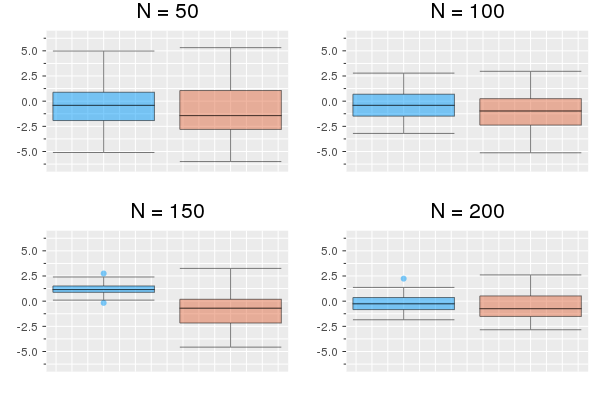
O–U: Experiment 3. To compare the efficiency of Constructs 1 and 2 for the case of jump processes, as developed in Section 3.2, we applied Algorithm 2 – for each case – to approximate the score function (at the true values for ), with particles, with data generated from O–U process (6.1) with fixed , , and true remaining parameters . Fig. 6.3 shows boxplots summarising the results from replications of the obtained estimates. We note that performance of Construct 2 is, in this case, much better than that of Construct 1.


6.2 Periodic Drift SDE
We consider the (highly) nonlinear model,
| (6.2) |
for , . We used true values , generated data, and applied Algorithm 3 with particles and initial values . To illustrate the mesh-free performance of Algorithm 3, we choose two values, and and compare the obtained numerical results. Figure 6.4 shows the data (Left Panel) and the trajectory of the estimated parameter values (Right Panel). Note that the SDE in (6.2) is making infrequent jumps between a number of modes. Indeed, in this case, the results are stable when increasing from to .

6.3 Heston Model
Consider the Heston model (Heston,, 1993), for price and volatility , modelled as,
where , are independent standard Brownian motions. Define the log-price , so that application of Itô’s lemma gives,
| (6.3) |
We make the standard assumption , so that the CIR process will not hit ; also, we have . Process is observed at discrete times, so that , . Thus, we have,
where we have set,
We chose true parameter value , and generated observations, with . We applied Algorithm 3 with and particles. The trajectories of the estimated parameters are given in Figure 6.5.

6.4 Sequential Model Selection – Real Data
We use our methodology to carry out sequential model selection, motivated by applications in Eraker et al., (2003); Johannes et al., (2009). Recall that BIC (Schwarz,, 1978) for model , with parameter vector , and data is given by,
where denotes the MLE, and the log-likelihood. BIC and the (closely related) Bayes Factor are known to have good asymptotic properties, e.g. they are consistent Model Selection Criteria, under the assumption of model-correctness, in the context of nested models, for specific classes of models (see e.g. Chib and Kuffner, (2016); Nishii, (1988); Sin and White, (1996), and Yonekura et al., (2018) for the case of discrete-time nested HMMs). One can plausibly conjecture such criteria will also perform well for the type of continuous-time HMMs we consider here. See also Eguchi and Masuda, (2018) for a rigorous analysis of BIC for diffusion-type models. Given models , with , we use the difference,
with involved terms defined as obviously, to choose between and .
We note that Eraker et al., (2003) use Bayes Factor for model selection in the context of SDE processes; that work uses MCMC to estimate parameters, and is not sequential (or online). We stress that our methodology allows for carrying out inference for parameters and the signal part of the model, and simultaneously allowing for model selection, all in an online fashion. Also, it is worth noting that Johannes et al., (2009) use the sequential likelihood ratio for model comparison, but such quantity can overshoot, i.e. the likelihood ratio will tend to choose a large model. Also, that work uses fixed calibrated parameters, so it does not relate to online parameter inference.
Remark 5.
We will use the running estimate of the parameter vector as a proxy for the MLE given the data already taken under consideration. Similarly, we use the weights of the particle filter to obtain a running proxy of the log-likelihood evaluated at the MLE, thus overall an online approximation of BIC. Such an approach, even not fully justified theoretically, can provide reasonable practical insights when performing model comparison in an online manner – particularly so, given when there is no alternative, to the best of our knowledge, for such an objective.
We consider the following family of nested SDE models,
where,
Such models have been used for short-term interest rates; see Jones, (2003); Durham, (2003); Aït-Sahalia, (1996); Bali and Wu, (2006) and references therein for more details. Motivated by Dellaportas et al., (2006); Stanton, (1997), we applied our methodology to daily 3-month Treasury Bill rates, from 2nd of January 1970, to 29th of December 2000, providing observations. The data can be obtained from the Federal Reserve Bank of St. Louis, at webpage https://fred.stlouisfed.org/series/TB3MS. The dataset is shown at Fig. 6.6.

Fig. 6.7 shows the BIC differences, obtained online, for each of the three pairs of models. The results suggest that does not provide a good fit to the data – relatively to , – for almost all period under consideration. In terms of against , there is evidence that once the data from around 1993 onwards are taken under consideration, is preferred to . In general, one can claim that models with non-linear drift should be taken under consideration for fitting daily 3-month Treasury Bill rates, without strong evidence in favour or against linearity. This non-definite conclusion is in some agreement with the empirical studies in Chapman and Pearson, (2000); Durham, (2003); Dellaportas et al., (2006).

7 Conclusions and Future Directions
We have introduced an online particle smoothing methodology for discretely observed (jump) diffusions with intractable transition densities. Our approach overcomes such intractability by formulating the problem on pathspace, thus delivering an algorithm that – besides regulatory conditions – requires only the weak invertibility Assumption 2. Thus, we have covered a rich family of SDE models, when related literature imposes quite strong restrictions. Combining our online smoothing algorithm with a Robbins-Monro-type approach of Recursive Maximum-Likelihood, we set up an online stochastic gradient-ascent for the likelihood function of the SDEs under consideration. The algorithm provides a wealth of interesting output, that can provide a lot of useful insights in statistical applications. The numerical examples show a lot of promise for the performance of the methodology. Our framework opens up a number of routes for insights and future research, including the ones described below.
-
(i)
In the case of SDEs of jumps, we have focused on jump dynamics driven by compound Poisson processes. There is great scope for generalisation here, and one can extend the algorithm to different cases of jump processes, also characterised by more complex dependencies between the jumps and the paths of the solution of the SDE, . Extensions to time-inhomogeneous cases with , , are immediate; we have chosen the time-homogeneous models only for purposes of presentation simplicity.
-
(ii)
Since the seminal work of Delyon and Hu, (2006), more ‘tuned’ auxiliary bridge processes have appeared in the literature, see e.g. the works of Schauer et al., (2017); van der Meulen and Schauer, (2017). Indicatively, the work in Schauer et al., (2017) considers bridges of the form (in one of the many options they consider),
(7.1) Auxiliary bridge processes that are closer in dynamics to the diffusion bridges of the given signal are expected to reduce the variability of Monte-Carlo algorithm, thus progress along the above direction can be immediately incorporated in our methodology and improve its performance. For instance, as noted in Schauer et al., (2017), use of (7.1) will give a Radon-Nikodym derivative where stochastic integrals cancel out. Such a setting is known to considerably reduce the variability of Monte-Carlo methods, see e.g. the numerical examples in Durham and Gallant, (2002) and the discussion in (Papaspiliopoulos and Roberts,, 2012, Section 4).
-
(iii)
The exact specification of the recursion used for the online estimation of unknown parameters is in itself an problem of intensive research in the field of stochastic optimisation. One would ideally aim for the recursion procedure to provide parameter estimates which are as close to the unknown parameter as the data (considered thus far) permit. In our case, we have used a fairly ‘vanilla’ recursion, maybe with the exception of the Adam variation. E.g., recent works in the Machine Learning community have pointed at the use of ‘velocity’ components in the recursion to speed up convergence, see, e.g., Sutskever et al., (2013); Yuan et al., (2016).
-
(iv)
We mentioned in the main text several modifications that can improve algorithmic performance: dynamic resampling, stratified resampling, non-blind proposals in the filtering steps, choice of auxiliary processes. Parallelisation and use of HPC are obvious additions in this list.
-
(v)
We stress that the algorithm involves a filtering step, and a step that approximates the values of the instrumental function. These two procedures should be thought of separately. One reason for including two approaches in the case of jump diffusions (Constructs 1 and 2) is indeed to highlight this point. The two Constructs are identical in terms of the filtering part. Construct 1 incorporates in the location of the path at all times of jumps; thus, when the algorithm ‘mixes’ all pairs of , , at the update of the instrumental function (see Step (iv) of Algorithm 2), many of such pairs can be incompatible (simply consider any such pair with , when has in fact been generated conditionally on ). Such an effect is even stronger in the case of the standard algorithm applied in the motivating example in the Introduction, and partially explains the inefficiency of that algorithm. In contrast, in Construct 2, contains less information about the underlying paths, thereby improving the compatibility of pairs selected from particle populations , , thus – not surprisingly – Construct 2 seems more effective than Construct 1.
-
(vi)
The experiments included in Section 6 of the paper aim to highlight the qualitative aspects of the introduced approach. The key property of robustness to mesh-refinement underlies all numerical applications, and is explicitly illustrated in the experiment in Section 6.2, and within Figure 6.4. In all cases, the code was written in Julia, was not parallelised or optimised and was run on a PC, with executions times that were quite small due to the online nature of the algorithm (the most expensive experiment took about 30 minutes). We have avoided a comparison with potential alternative approaches as we believe this would obscure the main messages we have tried to convey within the numerical results section. Such a detailed numerical study can be the subject of future work.
Acknowledgments
We are grateful to the AE and the referees for several useful comments that helped us to improve the content of the paper.
References
- Aït-Sahalia, (1996) Aït-Sahalia, Y. (1996). Testing continuous-time models of the spot interest rate. The Review of Financial Studies, 9(2):385–426.
- Aït-Sahalia, (2002) Aït-Sahalia, Y. (2002). Maximum likelihood estimation of discretely sampled diffusions: a closed-form approximation approach. Econometrica, 70(1):223–262.
- Aït-Sahalia, (2008) Aït-Sahalia, Y. (2008). Closed-form likelihood expansions for multivariate diffusions. The Annals of Statistics, 36(2):906–937.
- Aït-Sahalia et al., (2005) Aït-Sahalia, Y., Mykland, P. A., and Zhang, L. (2005). How often to sample a continuous-time process in the presence of market microstructure noise. The Review of Financial Studies, 18(2):351–416.
- Aït-Sahalia and Yu, (2008) Aït-Sahalia, Y. and Yu, J. (2008). High frequency market microstructure noise estimates and liquidity measures. Technical report, National Bureau of Economic Research.
- Andrieu et al., (2010) Andrieu, C., Doucet, A., and Holenstein, R. (2010). Particle Markov Chain Monte Carlo methods. Journal of the Royal Statistical Society: Series B (Statistical Methodology), 72(3):269–342.
- Azuma, (1967) Azuma, K. (1967). Weighted sums of certain dependent random variables. Tohoku Mathematical Journal, Second Series, 19(3):357–367.
- Bali and Wu, (2006) Bali, T. G. and Wu, L. (2006). A comprehensive analysis of the short-term interest-rate dynamics. Journal of Banking & Finance, 30(4):1269–1290.
- Beskos et al., (2006) Beskos, A., Papaspiliopoulos, O., Roberts, G. O., and Fearnhead, P. (2006). Exact and computationally efficient likelihood-based estimation for discretely observed diffusion processes (with discussion). Journal of the Royal Statistical Society: Series B (Statistical Methodology), 68(3):333–382.
- Cappe, (2009) Cappe, O. (2009). Online sequential Monte Carlo EM algorithm. In 2009 IEEE/SP 15th Workshop on Statistical Signal Processing.
- Cappé et al., (2005) Cappé, O., Moulines, E., and Ryden, T. (2005). Inference in Hidden Markov Models. Springer Science & Business Media.
- Carpenter et al., (1999) Carpenter, J., Clifford, P., and Fearnhead, P. (1999). Improved particle filter for nonlinear problems. IEE Proceedings-Radar, Sonar and Navigation, 146(1):2–7.
- Chapman and Pearson, (2000) Chapman, D. A. and Pearson, N. D. (2000). Is the short rate drift actually nonlinear? The Journal of Finance, 55(1):355–388.
- Chib and Kuffner, (2016) Chib, S. and Kuffner, T. A. (2016). Bayes factor consistency. arXiv preprint, arXiv:1607.00292.
- Chib et al., (2004) Chib, S., Pitt, M. K., and Shephard, N. (2004). Likelihood based inference for diffusion driven models.
- Chopin et al., (2013) Chopin, N., Jacob, P. E., and Papaspiliopoulos, O. (2013). SMC2: an efficient algorithm for sequential analysis of state space models. Journal of the Royal Statistical Society: Series B (Statistical Methodology), 75(3):397–426.
- Dahlhaus and Neddermeyer, (2010) Dahlhaus, R. and Neddermeyer, J. C. (2010). Particle filter-based on-line estimation of spot volatility with nonlinear market microstructure noise models. arXiv preprint arXiv:1006.1860.
- Del Moral et al., (2010) Del Moral, P., Doucet, A., and Singh, S. (2010). Forward smoothing using sequential Monte Carlo. arXiv preprint arXiv:1012.5390.
- Dellaportas et al., (2006) Dellaportas, P., Friel, N., and Roberts, G. O. (2006). Bayesian model selection for partially observed diffusion models. Biometrika, 93(4):809–825.
- Delyon and Hu, (2006) Delyon, B. and Hu, Y. (2006). Simulation of conditioned diffusion and application to parameter estimation. Stochastic Processes and their Applications, 116(11):1660–1675.
- Douc et al., (2011) Douc, R., Garivier, A., Moulines, E., and Olsson, J. (2011). Sequential Monte Carlo smoothing for general state space hidden Markov models. The Annals of Applied Probability, 21(6):2109–2145.
- Douc et al., (2014) Douc, R., Moulines, E., and Stoffer, D. (2014). Nonlinear time series: Theory, methods and applications with R examples. Chapman and Hall/CRC.
- Doucet et al., (2000) Doucet, A., Godsill, S., and Andrieu, C. (2000). On sequential Monte Carlo sampling methods for Bayesian filtering. Statistics and Computing, 10(3):197–208.
- Durham, (2003) Durham, G. B. (2003). Likelihood-based specification analysis of continuous-time models of the short-term interest rate. Journal of Financial Economics, 70(3):463–487.
- Durham and Gallant, (2002) Durham, G. B. and Gallant, A. R. (2002). Numerical techniques for maximum likelihood estimation of continuous-time diffusion processes. Journal of Business & Economic Statistics, 20(3):297–338.
- Eguchi and Masuda, (2018) Eguchi, S. and Masuda, H. (2018). Schwarz type model comparison for LAQ models. Bernoulli, 24(3):2278–2327.
- Eraker et al., (2003) Eraker, B., Johannes, M., and Polson, N. (2003). The impact of jumps in volatility and returns. The Journal of Finance, 58(3):1269–1300.
- Fearnhead et al., (2008) Fearnhead, P., Papaspiliopoulos, O., and Roberts, G. O. (2008). Particle filters for partially observed diffusions. Journal of the Royal Statistical Society: Series B (Statistical Methodology), 70(4):755–777.
- Gloaguen et al., (2018) Gloaguen, P., Étienne, M.-P., and Le Corff, S. (2018). Online sequential Monte Carlo smoother for partially observed diffusion processes. EURASIP Journal on Advances in Signal Processing, 2018(1):9.
- Golightly and Wilkinson, (2008) Golightly, A. and Wilkinson, D. J. (2008). Bayesian inference for nonlinear multivariate diffusion models observed with error. Computational Statistics & Data Analysis, 52(3):1674–1693.
- Gonçalves and Roberts, (2014) Gonçalves, F. B. and Roberts, G. O. (2014). Exact simulation problems for jump-diffusions. Methodology and Computing in Applied Probability, 16(4):907–930.
- Goodfellow et al., (2016) Goodfellow, I., Bengio, Y., and Courville, A. (2016). Deep Learning. MIT press.
- Gordon et al., (1993) Gordon, N. J., Salmond, D. J., and Smith, A. F. (1993). Novel approach to nonlinear/non-gaussian bayesian state estimation. In IEE Proceedings F (Radar and Signal Processing), volume 140, pages 107–113. IET.
- Hansen and Scheinkman, (1993) Hansen, L. P. and Scheinkman, J. A. (1993). Back to the future: Generating moment implications for continuous-time Markov processes. Technical report, National Bureau of Economic Research.
- Hansen and Lunde, (2006) Hansen, P. R. and Lunde, A. (2006). Realized variance and market microstructure noise. Journal of Business & Economic Statistics, 24(2):127–161.
- Heston, (1993) Heston, S. L. (1993). A closed-form solution for options with stochastic volatility with applications to bond and currency options. The Review of Financial Studies, 6(2):327–343.
- Johannes et al., (2009) Johannes, M. S., Polson, N. G., and Stroud, J. R. (2009). Optimal filtering of jump diffusions: Extracting latent states from asset prices. The Review of Financial Studies, 22(7):2759–2799.
- Jones, (2003) Jones, C. S. (2003). Nonlinear mean reversion in the short-term interest rate. The Review of Financial Studies, 16(3):793–843.
- Kalogeropoulos et al., (2010) Kalogeropoulos, K., Roberts, G. O., and Dellaportas, P. (2010). Inference for stochastic volatility models using time change transformations. The Annals of Statistics, 38(2):784–807.
- Kantas et al., (2015) Kantas, N., Doucet, A., Singh, S. S., Maciejowski, J., and Chopin, N. (2015). On particle methods for parameter estimation in state-space models. Statistical Science, 30(3):328–351.
- Kessler, (1997) Kessler, M. (1997). Estimation of an ergodic diffusion from discrete observations. Scandinavian Journal of Statistics, 24(2):211–229.
- Kessler et al., (2012) Kessler, M., Lindner, A., and Sorensen, M. (2012). Statistical methods for stochastic differential equations. Chapman and Hall/CRC.
- Kessler and Sørensen, (1999) Kessler, M. and Sørensen, M. (1999). Estimating equations based on eigenfunctions for a discretely observed diffusion process. Bernoulli, 5(2):299–314.
- Kingma and Ba, (2014) Kingma, D. P. and Ba, J. (2014). Adam: A method for stochastic optimization. arXiv preprint arXiv:1412.6980.
- Kitagawa, (1987) Kitagawa, G. (1987). Non-gaussian state space modeling of nonstationary time series. Journal of the American Statistical Association, 82(400):1032–1041.
- Kitagawa, (1996) Kitagawa, G. (1996). Monte Carlo filter and smoother for non-Gaussian nonlinear state space models. Journal of Computational and Graphical Statistics, 5(1):1–25.
- Kloeden and Platen, (2013) Kloeden, P. E. and Platen, E. (2013). Numerical solution of stochastic differential equations, volume 23. Springer Science & Business Media.
- LeGland and Mevel, (1997) LeGland, F. and Mevel, L. (1997). Recursive estimation in hidden Markov models. In Decision and Control, 1997, Proceedings of the 36th IEEE Conference, volume 4, pages 3468–3473. IEEE.
- Nishii, (1988) Nishii, R. (1988). Maximum likelihood principle and model selection when the true model is unspecified. Journal of Multivariate Analysis, 27(2):392–403.
- Øksendal and Sulem, (2007) Øksendal, B. and Sulem, A. (2007). Applied Stochastic Control of Jump Diffusions. Springer Science & Business Media.
- Olsson and Westerborn, (2017) Olsson, J. and Westerborn, J. (2017). Efficient particle-based online smoothing in general hidden Markov models: the PaRIS algorithm. Bernoulli, 23(3):1951–1996.
- Papaspiliopoulos and Roberts, (2012) Papaspiliopoulos, O. and Roberts, G. (2012). Importance sampling techniques for estimation of diffusion models. Statistical methods for stochastic differential equations, 124:311–340.
- Papaspiliopoulos et al., (2013) Papaspiliopoulos, O., Roberts, G. O., and Stramer, O. (2013). Data augmentation for diffusions. Journal of Computational and Graphical Statistics, 22(3):665–688.
- Poyiadjis et al., (2011) Poyiadjis, G., Doucet, A., and Singh, S. S. (2011). Particle approximations of the score and observed information matrix in state space models with application to parameter estimation. Biometrika, 98(1):65–80.
- Reddi et al., (2019) Reddi, S. J., Kale, S., and Kumar, S. (2019). On the convergence of Adam and beyond. arXiv preprint arXiv:1904.09237.
- Roberts and Stramer, (2001) Roberts, G. O. and Stramer, O. (2001). On inference for partially observed nonlinear diffusion models using the Metropolis–Hastings algorithm. Biometrika, 88(3):603–621.
- Särkkä and Sottinen, (2008) Särkkä, S. and Sottinen, T. (2008). Application of Girsanov theorem to particle filtering of discretely observed continuous-time non-linear systems. Bayesian Analysis, 3(3):555–584.
- Schauer et al., (2017) Schauer, M., Van Der Meulen, F., and Van Zanten, H. (2017). Guided proposals for simulating multi-dimensional diffusion bridges. Bernoulli, 23(4A):2917–2950.
- Schwarz, (1978) Schwarz, G. (1978). Estimating the dimension of a model. Annals of Statistics, 6(2):461–464.
- Sin and White, (1996) Sin, C.-Y. and White, H. (1996). Information criteria for selecting possibly misspecified parametric models. Journal of Econometrics, 71(1-2):207–225.
- Stanton, (1997) Stanton, R. (1997). A nonparametric model of term structure dynamics and the market price of interest rate risk. The Journal of Finance, 52(5):1973–2002.
- Ströjby and Olsson, (2009) Ströjby, J. and Olsson, J. (2009). Efficient particle-based likelihood estimation in partially observed diffusion processes. IFAC Proceedings Volumes, 42(10):1364–1369.
- Sutskever et al., (2013) Sutskever, I., Martens, J., Dahl, G., and Hinton, G. (2013). On the importance of initialization and momentum in Deep Learning. In International Conference on Machine Learning, pages 1139–1147.
- Tadic and Doucet, (2018) Tadic, V. Z. and Doucet, A. (2018). Asymptotic properties of recursive maximum likelihood estimation in non-linear state-space models. arXiv preprint arXiv:1806.09571.
- van der Meulen and Schauer, (2017) van der Meulen, F. and Schauer, M. (2017). Bayesian estimation of discretely observed multi-dimensional diffusion processes using guided proposals. Electronic Journal of Statistics, 11(1):2358–2396.
- Wagner, (1989) Wagner, W. (1989). Undiased Monte Carlo estimators for functionals of weak solutions of stochastic differential equations. Stochastics: An International Journal of Probability and Stochastic Processes, 28(1):1–20.
- Yonekura et al., (2018) Yonekura, S., Beskos, A., and Singh, S. (2018). Asymptotic analysis of model selection criteria for general hidden Markov models. arXiv preprint arXiv:1811.11834.
- Yuan et al., (2016) Yuan, K., Ying, B., and Sayed, A. H. (2016). On the influence of momentum acceleration on online learning. The Journal of Machine Learning Research, 17(1):6602–6667.
Appendix A Proof of Proposition 1
Proof.
We have the integral,
| (A.1) |
Also, simple calculations give,
Using this expression in the integral on the right side of (A.1) completes the proof. ∎
Appendix B Proof of Proposition 2
Proof.
Simply note that,
Then, we have that,
Replacing the probability measure on the left side of the above equality with its equal on the right side, and using the latter in the integral above completes the proof for the first equation in the statement of the proposition. The second equation follows from trivial use of Bayes rule. ∎
Appendix C Proof of Proposition 3
Proof.
Part (i) follows via the same arguments as in Olsson and Westerborn, (2017, Corollary 2), based on Azuma, (1967) and Douc et al., (2011, Lemma 4). For part (ii), one can proceed as follows. Given , we define the event , where we added superscript to stress the dependency of the estimate on the number of particles. Then,
| (C.1) |
From (i), we get , so . The Borel–Cantelli lemma gives , therefore the result follows from (C.1). ∎