Online Market Equilibrium with Application to Fair Division
Abstract
Computing market equilibria is a problem of both theoretical and applied interest. Much research to date focuses on the case of static Fisher markets with full information on buyers’ utility functions and item supplies. Motivated by real-world markets, we consider an online setting: individuals have linear, additive utility functions; items arrive sequentially and must be allocated and priced irrevocably. We define the notion of an online market equilibrium in such a market as time-indexed allocations and prices which guarantee buyer optimality and market clearance in hindsight. We propose a simple, scalable and interpretable allocation and pricing dynamics termed as PACE. When items are drawn i.i.d. from an unknown distribution (with a possibly continuous support), we show that PACE leads to an online market equilibrium asymptotically. In particular, PACE ensures that buyers’ time-averaged utilities converge to the equilibrium utilities w.r.t. a static market with item supplies being the unknown distribution and that buyers’ time-averaged expenditures converge to their per-period budget. Hence, many desirable properties of market equilibrium-based fair division such as no envy, Pareto optimality, and the proportional-share guarantee are also attained asymptotically in the online setting. Next, we extend the dynamics to handle quasilinear buyer utilities, which gives the first online algorithm for computing first-price pacing equilibria. Finally, numerical experiments on real and synthetic datasets show that the dynamics converges quickly under various metrics.
1 Introduction
A market is said to be in equilibrium when supply is equal to demand. Computing prices and allocations which constitute a market equilibrium (ME) has long been a topic of interest [43, 28, 38, 20, 17, 31]. Most existing work focuses on the case of static markets. However, in this paper we consider the case of online markets where items arrive sequentially. We consider the extension of market equilibrium to this setting and provide market dynamics which quickly converge to an equilibrium in the case of online Fisher markets.
In static Fisher markets there is a fixed supply of each item, individual preferences are linear, additive, and items are divisible (or equivalently, randomization is allowed so individuals can purchase not just items but lotteries over items). In general, finding market equilibria is a hard problem [14, 47, 39]. However, in static linear Fisher markets, equilibrium prices and allocations can be computed via solving the Eisenberg-Gale (EG) convex program [22, 37].
We consider an online extension of Fisher markets where buyers are constantly present but items arrive one-at-a-time. Buyers’ budgets are per-period and represent their respective ‘bidding powers’ instead of being binding constraints. We extend the definition of market equilibrium to the online setting: online equilibrium allocations and prices are time-indexed and, when averaged across time, form an equilibrium in a corresponding static Fisher market where item supplies are proportional to item arrival probabilities. Due to the stochastic nature of online Fisher markets, any online algorithm can only attain an online market equilibrium asymptotically, that is, the allocations and prices approximately satisfy the equilibrium conditions after running the algorithm for a long time.
We propose market dynamics that find these equilibria in an online fashion based on the dual averaging algorithm applied to a reformulation of the dual of the EG convex program. We refer to this mechanism as PACE (Pace According to Current Estimated utility). In PACE, each buyer is assigned a utility pacing multiplier at time . When an item arrives, the individual with the highest adjusted utility (its valuation times the multiplier) receives that item and pays a price equal to its adjusted utility. The pacing multipliers of all individuals are then adjusted according to a closed-form rule which is given by the time average of the subgradient of the dual of the EG program. Intuitively, the pacing multipliers of those that did not receive the item go up while the receiver’s typically (but not always) goes down. We show that PACE yields item allocations and prices that satisfy various equilibrium properties asymptotically, for example no-regret and envy-freeness.
One important application of market equilibrium is fair allocation using the competitive equilibrium from equal incomes (CEEI) mechanism [46, 12]. In CEEI, each individual is given an endowment of faux currency and reports her valuations for items; then, a market equilibrium is computed and the items are allocated accordingly. However, many fair division problems are online rather than static. These include the allocation of impressions to content in certain recommender systems [34], workers to shifts, donations to food banks [2], scarce compute time to requestors [25, 40, 29], or blood donations to blood banks [32]. Similarly, online advertising can also be thought of as the allocation of impressions to advertisers via a market though with a budget of real money rather than faux currency. In the static CEEI case with linear additive preferences, the resulting equilibrium outcomes (i.e. results of the EG program) have been described as “perfect justice” [3]. In the online case, PACE achieves the same fair allocations as CEEI asymptotically. See Appendix A for more related work in the areas of (static and online) equilibrium computation and fair division.
We evaluate PACE experimentally in several market datasets. Convergence to good outcomes happens quickly in experiments. Taken together our results, we conclude that PACE is an attractive algorithm for both computing online market equilibria and online fair division.
Main contributions.
We consider the problem of allocating and pricing sequentially arriving items to buyers. This setting is termed as an online Fisher market. Given a sequence of item arrivals, we define an online market equilibrium as the items’ allocations and prices that, in hindsight, ensure buyer optimality and market clearance. We propose the PACE dynamics, which can be viewed as a nontrivial instantiation of the dual averaging algorithm on a reformulation of the dual of the Eisenberg-Gale convex program. Leveraging the convergence theory of dual averaging, we show that, when item arrivals are drawn from an (unknown) underlying distribution , possibly over an infinite/continuous item space, PACE ensures the following.
-
•
The pacing multipliers generated by PACE converge to the static equilibrium utility prices. Here, “static” means w.r.t. to an underlying static Fisher market.
-
•
Buyers’ time-averaged utilities converge to the static equilibrium utilities.
-
•
Buyers’ time-averaged expenditures converge to their respective budgets.
These convergences are all in mean square with rates , and , respectively, where the constants in these rates involve moderate polynomials of . In this way, PACE generates allocations and prices that constitute an online market equilibrium in the limit. In particular, the allocations and prices ensure that the allocation is Pareto optimal, and buyers have no regret, no envy, and get at least their proportional share asymptotically. We also extend PACE to the case of quasilinear buyer utilities, which yields the first online algorithm for computing first-price pacing equilibria. Finally, numerical experiments suggest that PACE converges much faster than its theoretical rates in terms of pacing multipliers, utilities and expenditures.
2 Static and Online Fisher Markets
Static Fisher markets and equilibria.
We first introduce static Fisher markets and their equilibria. Following the recent work [24, §2], we consider a measurable (possibly continuous) item space. Below are the technical preliminaries for the subsequent online setting. They can be skimmed through and referred back to as needed.
From now on, we define for any and (, resp.) as the set of nonnegative (positive, resp.) real numbers. Let denote the indicator function of an event .
-
(a)
There are buyers (individuals), each having a budget .
-
(b)
The item space is a finite measurable space with , where is a (-)measurable subset of , is a -algebra and is a (finite) measure. From now on, (and , resp.) denote the set of (nonnegative, resp.) functions on for any (including ). Below are some concrete special cases for illustration.
-
(i)
Finite: , and (all subsets are measurable and the measure is given by a point mass on each item).
-
(ii)
Lebesgue-measurable: is the Lebesgue measure on , is the Lebesgue -algebra and is a (Lebesgue-)measurable subset of with positive finite measure. For example, can be a compact subset of with a nonempty interior.
-
(iii)
Countably infinite: and for any , where . For example, can be the probability mass of a Poisson distribution, in which case is a probability space.
-
(i)
-
(c)
The supplies of items is , i.e., item has supply . Since is compact, it is measurable with a finite measure. For the finite case , we have .
-
(d)
The valuation of each buyer on all items is , i.e., buyer has valuation on item . For the finite case , we have .
-
(e)
For buyer , an allocation of items gives a utility of
where the angle brackets are based on the notation of applying a bounded linear functional to a vector in the Banach space and the integral is the usual Lebesgue integral. For the finite case , we have and the utility is
the usual Euclidean vector inner product. We will use to denote the aggregate allocation of items to all buyers, i.e., the concatenation of all buyers’ allocations.
-
(f)
The prices of items are modeled as ; in other words, the price of item is . For the finite case , we have .
-
(g)
For a measurable item subset , let (and similarly for and ), the -induced measure of . For the finite case , for any item subset , (and similarly for and ).
-
(h)
Without loss of generality, we assume a unit total budget , a unit total supply and normalized buyer valuations . In other words, all items have a total value of for every buyer.
Definition 1.
Given item prices , the demand of buyer is its set of utility-maximizing allocations given the prices and budget:
The associated utility level is defined as the value of for any .
Definition 2.
A market equilibrium (ME) is an allocation-price pair such that the following holds.
-
(i)
Supply feasibility: .
-
(ii)
Buyer optimality: for all .
-
(iii)
Market clearance: (any item with a positive price is fully allocated).
In the above definition and subsequently, all equations involving measurable functions are understood as “holding almost everywhere.” For example, means the (measurable) set has the same measure as . Given a ME , we often denote the (unique) equilibrium utilities as . For a finite-dimensional linear Fisher market, it is well known that a ME can be computed via solving the EG convex program. Recently, [24] generalized this framework to handle the case of an infinite item space. More specifically, consider the following (possibly infinite-dimensional) convex programs.
| () |
| () | ||||
The following theorem summarizes the results in [24, §3] regarding the above convex programs capturing market equilibria. As shown in that work, the above convex programs satisfy strong duality and their optimal solutions (which correspond to ME) can be characterized by the KKT optimality conditions. We slightly generalize the assumptions of [24] by allowing non-uniform item supplies instead of for all . For completeness, a proof, which is mainly based on the proofs of the results in [24, §3], can be found in the Appendix.
In the above theorem, is known as buyer ’s utility price, i.e., price per unit utility at equilibrium. As is well known, in a ME , the allocations are
-
•
Pareto optimal,
-
•
envy-free (in a budget weighted sense, i.e., for all ),
-
•
proportional (i.e., ); see, e.g.,[24, Theorem 3].
Online Fisher markets and equilibria.
We now consider a simple online variant of the Fisher market setting, referred to as an online Fisher market (OFM). There are buyers, each with a valuation . Assume there are discrete time steps . At each time step , an item arrives and each buyer sees a value . The item must be allocated irrevocably to one buyer. Each buyer has a budget representing her per-period expenditure rate. 111This assumption is similar to one made in the literature on budget management in auctions, where each buyers has a per-period expenditure rate and the overall budget equal to the rate times the number of time periods. If a hard budget cap across all time periods is desired, then PACE and similar mechanisms may deplete some buyers’ budgets close to the end of the horizon [8, 6, 7].
Next, we introduce the notions of demand, utility level and online market equilibrium in an OFM. All of them are defined based on sequences of arrived items and their prices; they do not require any distributional assumption on the item arrivals.
Definition 3.
Let the arrived items be . An allocation (of arrived items) is , where is the fraction of the item allocated to buyer .222We allow fractional allocations in the definition for more generality. As we will see, fractional allocation is not needed: PACE generates allocations and prices that satisfy the OME conditions asymptotically via assigning each arrived item to one buyer. Let the prices of the arrived items be . The demand of each buyer (in hindsight) at time is
| (1) |
Let be the utility level associated with this demand, i.e., the maximum value in (1). An online market equilibrium (OME) is a pair of allocations and prices such that the following holds.
-
(i)
Total allocation does not exceed the unit amount of the item for all .
-
(ii)
Buyers’ realized allocations are optimal in hindsight: for all .
-
(iii)
Market clearance: for such that .
In words, is the maximum possible (time-averaged) utility buyer could have attained via choosing from the arrived items in hindsight, subject to their respective posted prices and her current total budget , with being the set of such utility-maximizing (time-indexed) allocations subject to per-period item availability constraints. An OME is a pair of allocations and prices that make buyers optimal in hindsight and market cleared.
Given an OFM, we define the associated underlying static Fisher market as having the same buyers and an item space with supply being the (unknown) distribution from which the arriving items are drawn. To clarify the concepts of OFM and OME, we consider some simple special cases.
-
•
Suppose all item arrivals are known in advance. Then, the OFM is the same as a static Fisher market with the same buyers and the items, each having a unit supply. Here, buyer ’s valuation of item is . To compute an OME, it suffices to solve the classical (finite-dimensional) Eisenberg-Gale convex program, that is, () with , and . Let the static ME be . When each item arrives, OME allocates a fraction of the item to each buyer and set its price as .
-
•
Suppose the sequentially arriving items are drawn i.i.d. from a known underlying distribution (which specifies a random variable such that for any measurable set ) and all buyers’ valuations are known. Suppose we have also computed a static ME (Definition 2) of a market with buyer valuations , budgets and item supplies being the distribution (the underlying static market). Then, when a new item (which is drawn from the distribution ) arrives at time , set its price as and allocate a fraction of it to each buyer (assume , i.e., only items with positive supplies can appear). Then, the time-averaged utility of each buyer is , which converges to
by to the Strong Law of Large Numbers. Since the online process is carried out using static equilibrium prices and allocations, the static ME properties (Definition 2) ensure the required OME properties hold asymptotically.
The above special cases require full knowledge of either the exact future item arrivals or the underlying static market to attain an OME. Next, we propose a simple, distributed dynamics which generates allocations and prices that satisfy the OME conditions asymptotically without requiring such knowledge (in particular, without knowledge of the distribution ).
3 The PACE Dynamics
In this section, we introduce the PACE (Pacing According to Current Estimated utility) dynamics that prices and allocates sequentially arriving items via (i) maintaining a pacing multiplier for each buyer and (ii) simple, distributed updates.333Pacing and pacing multipliers are terminology in budget management in large-scale ad auctions [18, 19]. In §5, we will show that PACE is an instantiation of dual averaging [48], a stochastic first-order method for regularized optimization, applied to a reformulation of ().
In the PACE dynamics, each buyer maintains a pacing multiplier (with an initial value , or any value in ). At time step , the following events take place.
-
(a)
An item appears and each buyer sees a value for the item.
-
(b)
Each buyer bids their paced value for the item.
-
(c)
The item is allocated to the highest bidder (the winner at ): , with ties broken arbitrarily. For concreteness, we always choose the lowest winning index, i.e.,
Then, the price of is set by the first-price rule
and the winner pays this price for the item .
-
(d)
Each buyer gets a utility
In other words, the winner gets and other buyers get zero.
-
(e)
Each buyer updates its cumulative average utility :
-
(f)
Each buyer updates their pacing multiplier as follows:
where and for some fixed (e.g., ).
As will be seen in §5, buyer ’s equilibrium pacing multiplier (utility price) satisfies and her per-period utility corresponds to the th component of a stochastic subgradient of a function on in a reformulation of the convex program (), on which we run dual averaging. Furthermore, the update rule for is such that, if the realized utilities were the true static equilibrium utility for buyer , then would be the equilibrium multiplier. Note that PACE does not randomize (any randomness can only come from the market environment from which item arrivals are drawn) and assigns every item to a single buyer without splitting it.
The simplicity and distributed nature of PACE makes it desirable for large-scale practical use.
-
•
It can be run on arbitrary sequential item arrivals and only requires buyers’ valuations on the arrived items (rather than all valuations over the potentially large item space). No parameter tuning is needed (in particular, no stepsize tuning as in many first-order optimization methods).
-
•
When run as a centralized allocation mechanism, PACE only needs to maintain scalars, namely, , and for all . At time , it observes buyers’ valuations of the item , compute bids , finds the winner , set the price as the maximal bid and allocates the item to the winner; finally, it updates and as in f, which takes time.
-
•
PACE can also be run among the buyers in a decentralized manner, in which case each buyer only maintains two scalar values: the pacing multiplier and time-averaged utility . When a new item arrives, each buyer only performs a few simple arithmetic operations to create a bid , receives her utility (if she wins) and subsequently updates and .
These make PACE suitable for Internet-scale online fair division and online Fisher market applications. In particular, it is very reminiscent of how Internet advertising auctions are run. There, a similar auction-based system is used, with the pacing multiplier ensuring that each advertiser smooths out their budget expenditure across the many auctions. The primary difference between this and our setting is that (i) the auction can be first-price or second-price and (ii) buyers usually have quasilinear utilities, that is, utility of the item minus the expenditure (price paid) [18, 8, 6, 7]. In §C, we extend PACE to quasilinear utilities, which provides a novel online algorithm for first-price pacing equilibrium computation [19].
4 Dual Averaging
In this section, we briefly recap the setup and general convergence results of dual averaging [48, 35], which will be used in the analysis of PACE. First, we introduce some notation for this and subsequent sections. Let denote the ’th unit basis vector in and denote the vector of ’s. For , denotes the Cartesian product of intervals . All norms without a subscript are Euclidean -norms, unless otherwise stated.
Let be a closed convex function with domain . Let be an arbitrary sample space. For each , let be a convex and subdifferentiable function on . Considers the following regularized convex optimization problem [48, §1.1]:
| (2) |
where the expectation is taken over a probability distribution on . A more general online optimization setting, as described in [48, §1.2] is as follows. At each time , we must choose an action before a new, unknown convex loss function arrives, which incurs a loss (a special case is i.i.d. sampled functions, i.e., , where are i.i.d. samples drawn from ). The goal is to minimize regret when comparing our sequence of actions to any fixed action . Here, the regret against is defined as
and the overall (maximal) regret up to time is . We assume access to an oracle that, given any and , returns a subgradient . The dual averaging algorithm (DA) [48, Algorithm 1] is as follows. First, set and . Then, for each , DA performs the following steps:
-
(1)
Observe and compute .
-
(2)
Update the average subgradient (the dual average) via .
-
(3)
Compute the next iterate .
Here, we do not employ any auxiliary regularizing function, since our problem has a natural source of strong convexity (i.e., a strongly convex ) through the terms in (). The following convergence guarantee on DA is proved as part of the proof of Corollary 4 in [48].
Theorem 2.
Dual averaging generates iterates such that
where is an upper bound on , and is the strong convexity modulus of .
When solving the stochastic optimization problem (2), in Theorem 2, we can set to be an upper bound on , where is a subgradient oracle mapping each to a subgradient and the expectation is over and possible randomness of the subgradient oracle. We will shortly see that a reformulation of , when cast into the form (2), exhibits stochastic subgradients that are exactly buyers’ received utilities in each time step. Using Theorem 2, we can show that the sequence of pacing multipliers generated by PACE converges to the underlying (equilibrium) utility prices of the static Fisher market.
5 Convergence analysis of the PACE dynamics
We will now show that PACE correspond to running DA on the vector of pacing multipliers for the buyers. To this end, we first reformulate () into a (finite-dimensional) convex program in in the form of (2):
| (3) |
where is an arbitrarily small constant. The bounds on do not change the optimal solution, because for each . Detailed steps of the reformulation are given in Appendix B.
In order to run DA, we need to compute a subgradient of at any . Following [24, §5], since is a piecewise linear function, a subgradient is
where is the winner (see, e.g., [10, Theorem 3.50]).
We can now show that the PACE dynamics corresponds to running DA on (3). First, choose an arbitrary and . At each time step , given the current pacing multiplier , DA applied to (3) unrolls the following steps.
-
•
An item arrives, having value for each buyer . The function in DA is
-
•
The winner is and a subgradient is
Its th entry is exactly the realized (single-period) utility of individual at time in PACE, that is, .
-
•
Update the dual average (time-averaged utilities): for each , compute , i.e.,
-
•
Update the pacing multipliers:
The minimization problem is separable in each and exhibits a simple and explicit solution which recovers step f in PACE (where ):
As mentioned earlier, PACE does not require a stepsize parameter. This is because DA is stepsize-free given a strongly convex regularizer , which is indeed the case in our reformulation (3). In addition, in the above update step for , the directions of change are as follows.
-
•
For a non-winner , we have and hence . This implies . In words, a non-winner’s pacing multiplier weakly increases. The increase is strict if , i.e., buyer has already received a nonzero utility.
-
•
For the winner , may become greater than , in which case . In words, the winner’s pacing multiplier may go up or down.
In order to analyze PACE, we assume , (normalized and a.e.-bounded valuations)444The a.e.-boundedness assumption is needed in subsequent convergence analysis. Since has a finite measure, it holds that . For a finite item space , both are equal to . and that there is an underlying item distribution from which the item arrivals , are drawn i.i.d.555The distributional assumption on item arrivals (i.e., they are drawn i.i.d. from an unknown distribution ) is needed to establish asymptotic equilibrium properties of PACE. See Appendix B for an example that any algorithm can yield arbitrarily suboptimal allocations without such a distributional assumption. Define the underlying static Fisher market as one having the same buyers (each with valuation and budget ) and item supplies . Denote the equilibrium utilities and utility prices w.r.t. the underlying static market as and , respectively. We further assume that the valuations are (i.e., a.e.-bounded on the item space). This is not restrictive: since an individual item has value for each buyer , it should be a finite value.
Convergence of pacing multipliers.
After aligning PACE with DA, the convergence of the pacing multipliers follows directly from Theorem 2.
Theorem 3.
PACE generates pacing multipliers , such that
where , .
In other words, we have mean-square convergence of to at a rate. Since , we have . Hence, and the constant in the bound is . Whether such dependence on can be improved via new analysis remains an interesting research question.
Convergence of utilities.
We next show that the time-averaged utility (which is equal to the dual average ) converges to the equilibrium utility vector of the underlying Fisher market. A key step in the proof is to bound the probability of a projection in updating , that is, .
Theorem 4.
For each , let be the minimum distance to the endpoints of the pacing-multiplier interval and . It holds that
Hence, letting , we have
Note that . Hence, in this and the next theorems, the constant in the bound is , which arises from and .
Convergence of expenditures.
The expenditure of buyer at time step is
In other words, only the winner spends a nonzero amount, which is its bid. Let be buyer ’s average expenditure. Utilizing the above convergence results, we show mean-squared convergence of to at an rate.
Theorem 5.
PACE attains OME asymptotically.
Next, we show that PACE attains OME asymptotically, i.e., it generates allocations and prices that make buyers no-regret and envy-free in the limit (these notions will be clarified shortly). Let denote whether buyer is the winner (i.e., whether she is allocated the item at time ) Utilizing Theorems 4 and 5, we can show that buyer ’s regret, that is, the difference between the maximum possible utility in hindsight (Definition 3) and the realized utility , vanishes as grows. The same holds for each buyer’s envy. In other words, at a large , in hindsight, no buyer prefers another buyer’s set of allocated items (up to a vanishing error).666In a static market, given an allocation , the (maximum, budget-weighted) envy of buyer toward others’ bundles is (see, e.g., [46, 12]). It is well-known that for all at equilibrium, a consequence of buyer optimality (Definition 2).
Theorem 6.
Denote
Let be the regret of buyer at time . Then, it holds that
Furthermore, let the envy of buyer (w.r.t. all other buyers) at time be
where is buyer ’s time-averaged utility given her own valuations and of buyer ’s allocations. Denote
It holds that
Hence, .
In light of Definition 3, Theorem 6 shows that is approximately optimal for buyer . Since PACE also clears the market, we conclude that it attains OME asymptotically. Recall that theorem 4 ensures that buyers’ converge to their static equilibrium utilities . Since the latter satisfy Pareto optimality and proportional share guarantee ( for all ), so are the time-averaged realized utilities in the limit. Together with Theorem 6, we conclude that PACE achieves the said fairness and efficiency guarantees, namely, Pareto optimality, envy-freeness and proportional-share guarantee, asymptotically.
6 Experiments
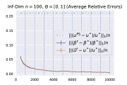
We evaluate the PACE dynamics in several real and synthetic datasets, namely, MovieLens, Household Items and an infinite-dimensional market instance with item space and being linear functions on . For the first two datasets, see [31] for more information and exploratory data analysis. For all datasets, we consider the CEEI (fair division) setting where for all . For each dataset (with number of buyers , respectively), we run PACE for time steps (iterations). More details on the experiments and additional plots displaying convergence of expenditures can be found in Appendix D. Figure 1 displays the mean values of the average and maximum relative errors of the pacing multipliers and time-averaged cumulative utilities over repeated experiments with different seeds (relative errors of cumulative spending w.r.t. total budgets are plotted separately in Appendix D). The standard errors are also displayed as vertical bars but are very small and nearly invisible. Vertical dotted lines indicate The figures do not show the initial iterates .
We see that PACE converges very quickly numerically: within epochs ( time steps) average deviations in most quantities falls within of the equilibrium quantity, with the worst case not far behind. An important point is that budget spend takes much longer to converge than utility. This demonstrates an important practical difference for using PACE in an allocation scenario where budgets are ‘real money’ (e.g. Internet ad impressions) as compared to a CEEI-like setting, where budgets are faux currency only used for fair division.
7 Conclusion
We introduced the concept of an online Fisher market and proposed the PACE dynamics. We showed that when items arrive sequentially and stochastically, PACE converges to equilibrium outcomes of the underlying market model. Furthermore, we showed that, as a consequence of this, PACE can be used in online fair division problems to generate an online allocation that, asymptotically, achieves the compelling fairness properties of CEEI.
Many questions remain for future research. We mostly focused on the case where budgets are faux currency and there are many open questions for adapting PACE to a real-money budget-management setting as well as more complicated nonlinear utility models. Another imperative question, especially for practitioners, is whether PACE guarantees some level of incentive-compatibility.


References
- Aleksandrov and Walsh [2020] M. Aleksandrov and T. Walsh. Online fair division: A survey. In Proceedings of the AAAI Conference on Artificial Intelligence, volume 34, pages 13557–13562, 2020.
- Aleksandrov et al. [2015] M. Aleksandrov, H. Aziz, S. Gaspers, and T. Walsh. Online fair division: Analysing a food bank problem. arXiv preprint arXiv:1502.07571, 2015.
- Arnsperger [1994] C. Arnsperger. Envy-freeness and distributive justice. Journal of Economic Surveys, 8(2):155–186, 1994.
- Azar et al. [2016] Y. Azar, N. Buchbinder, and K. Jain. How to allocate goods in an online market? Algorithmica, 74(2):589–601, 2016.
- Aziz et al. [2015] H. Aziz, S. Gaspers, S. Mackenzie, and T. Walsh. Fair assignment of indivisible objects under ordinal preferences. Artificial Intelligence, 227:71–92, 2015.
- Balseiro et al. [2017] S. Balseiro, A. Kim, M. Mahdian, and V. Mirrokni. Budget management strategies in repeated auctions. In Proceedings of the 26th International Conference on World Wide Web, pages 15–23, 2017.
- Balseiro and Gur [2019] S. R. Balseiro and Y. Gur. Learning in repeated auctions with budgets: Regret minimization and equilibrium. Management Science, 65(9):3952–3968, 2019.
- Balseiro et al. [2015] S. R. Balseiro, O. Besbes, and G. Y. Weintraub. Repeated auctions with budgets in ad exchanges: Approximations and design. Management Science, 61(4):864–884, 2015.
- Bateni et al. [2018] M. H. Bateni, Y. Chen, D. Ciocan, and V. Mirrokni. Fair resource allocation in a volatile marketplace. Available at SSRN 2789380, 2018.
- Beck [2017] A. Beck. First-order methods in optimization, volume 25. SIAM, 2017.
- Birnbaum et al. [2011] B. Birnbaum, N. R. Devanur, and L. Xiao. Distributed algorithms via gradient descent for fisher markets. In Proceedings of the 12th ACM conference on Electronic commerce, pages 127–136. ACM, 2011.
- Budish [2011] E. Budish. The combinatorial assignment problem: Approximate competitive equilibrium from equal incomes. Journal of Political Economy, 119(6):1061–1103, 2011.
- Caragiannis et al. [2016] I. Caragiannis, D. Kurokawa, H. Moulin, A. D. Procaccia, N. Shah, and J. Wang. The unreasonable fairness of maximum Nash welfare. In Proceedings of the 2016 ACM Conference on Economics and Computation, pages 305–322. ACM, 2016.
- Chen and Teng [2009] X. Chen and S.-H. Teng. Spending is not easier than trading: on the computational equivalence of fisher and arrow-debreu equilibria. In International Symposium on Algorithms and Computation, pages 647–656. Springer, 2009.
- Cheung et al. [2019] Y. K. Cheung, M. Hoefer, and P. Nakhe. Tracing equilibrium in dynamic markets via distributed adaptation. In Proceedings of the 18th International Conference on Autonomous Agents and MultiAgent Systems, pages 1225–1233, 2019.
- Cole and Gkatzelis [2018] R. Cole and V. Gkatzelis. Approximating the Nash social welfare with indivisible items. SIAM Journal on Computing, 47(3):1211–1236, 2018.
- Cole et al. [2017] R. Cole, N. R. Devanur, V. Gkatzelis, K. Jain, T. Mai, V. V. Vazirani, and S. Yazdanbod. Convex program duality, fisher markets, and Nash social welfare. In 18th ACM Conference on Economics and Computation, EC 2017. Association for Computing Machinery, Inc, 2017.
- Conitzer et al. [2018] V. Conitzer, C. Kroer, E. Sodomka, and N. E. Stier-Moses. Multiplicative pacing equilibria in auction markets. In International Conference on Web and Internet Economics, 2018.
- Conitzer et al. [2019] V. Conitzer, C. Kroer, D. Panigrahi, O. Schrijvers, E. Sodomka, N. E. Stier-Moses, and C. Wilkens. Pacing equilibrium in first-price auction markets. In Proceedings of the 2019 ACM Conference on Economics and Computation. ACM, 2019.
- Daskalakis et al. [2009] C. Daskalakis, P. W. Goldberg, and C. H. Papadimitriou. The complexity of computing a Nash equilibrium. SIAM Journal on Computing, 39(1):195–259, 2009.
- Dvoretzky et al. [1951] A. Dvoretzky, A. Wald, J. Wolfowitz, et al. Relations among certain ranges of vector measures. Pacific Journal of Mathematics, 1(1):59–74, 1951.
- Eisenberg and Gale [1959] E. Eisenberg and D. Gale. Consensus of subjective probabilities: The pari-mutuel method. The Annals of Mathematical Statistics, 30(1):165–168, 1959.
- Gao and Kroer [2020a] Y. Gao and C. Kroer. First-order methods for large-scale market equilibrium computation. In Neural Information Processing Systems 2020, NeurIPS 2020, 2020a.
- Gao and Kroer [2020b] Y. Gao and C. Kroer. Infinite-dimensional fisher markets and tractable fair division. arXiv preprint arXiv:2010.03025, 2020b.
- Ghodsi et al. [2011] A. Ghodsi, M. Zaharia, B. Hindman, A. Konwinski, S. Shenker, and I. Stoica. Dominant resource fairness: Fair allocation of multiple resource types. In Nsdi, volume 11, pages 24–24, 2011.
- Goldberg et al. [2001] K. Goldberg, T. Roeder, D. Gupta, and C. Perkins. Eigentaste: A constant time collaborative filtering algorithm. information retrieval, 4(2):133–151, 2001.
- Harper and Konstan [2015] F. M. Harper and J. A. Konstan. The movielens datasets: History and context. Acm transactions on interactive intelligent systems (tiis), 5(4):1–19, 2015.
- Kantorovich [1975] L. Kantorovich. Mathematics in economics: achievements, difficulties, perspectives. Technical report, Nobel Prize Committee, 1975.
- Kash et al. [2014] I. Kash, A. D. Procaccia, and N. Shah. No agent left behind: Dynamic fair division of multiple resources. Journal of Artificial Intelligence Research, 51:579–603, 2014.
- Kroer and Peysakhovich [2019] C. Kroer and A. Peysakhovich. Scalable fair division for ’at most one’ preferences. arXiv preprint arXiv:1909.10925, 2019.
- Kroer et al. [2019] C. Kroer, A. Peysakhovich, E. Sodomka, and N. E. Stier-Moses. Computing large market equilibria using abstractions. In Proceedings of the 2019 ACM Conference on Economics and Computation, pages 745–746, 2019.
- McElfresh et al. [2020] D. C. McElfresh, C. Kroer, S. Pupyrev, E. Sodomka, K. A. Sankararaman, Z. Chauvin, N. Dexter, and J. P. Dickerson. Matching algorithms for blood donation. In Proceedings of the 21st ACM Conference on Economics and Computation, pages 463–464, 2020.
- Murray et al. [2020a] R. Murray, C. Kroer, A. Peysakhovich, and P. Shah. Robust market equilibria with uncertain preferences. In Proceedings of the AAAI Conference on Artificial Intelligence, volume 34, pages 2192–2199, 2020a.
- Murray et al. [2020b] R. Murray, C. Kroer, A. Peysakhovich, and P. Shah. https://research.fb.com/blog/2020/09/robust-market-equilibria-how-to-model-uncertain-buyer-preferences/, Sep 2020b.
- Nesterov [2009] Y. Nesterov. Primal-dual subgradient methods for convex problems. Mathematical programming, 120(1):221–259, 2009.
- Nesterov and Shikhman [2018] Y. Nesterov and V. Shikhman. Computation of fisher–gale equilibrium by auction. Journal of the Operations Research Society of China, 6(3):349–389, 2018.
- Nisan et al. [2007] N. Nisan, T. Roughgarden, E. Tardos, and V. V. Vazirani. Algorithmic game theory. Cambridge University Press, 2007.
- Othman et al. [2010] A. Othman, T. Sandholm, and E. Budish. Finding approximate competitive equilibria: efficient and fair course allocation. In AAMAS, volume 10, pages 873–880, 2010.
- Othman et al. [2016] A. Othman, C. Papadimitriou, and A. Rubinstein. The complexity of fairness through equilibrium. ACM Transactions on Economics and Computation (TEAC), 4(4):1–19, 2016.
- Parkes et al. [2015] D. C. Parkes, A. D. Procaccia, and N. Shah. Beyond dominant resource fairness: Extensions, limitations, and indivisibilities. ACM Transactions on Economics and Computation (TEAC), 3(1):1–22, 2015.
- Peysakhovich and Kroer [2019] A. Peysakhovich and C. Kroer. Fair division without disparate impact. Mechanism Design for Social Good, 2019.
- Plaut and Roughgarden [2020] B. Plaut and T. Roughgarden. Almost envy-freeness with general valuations. SIAM Journal on Discrete Mathematics, 34(2):1039–1068, 2020.
- Scarf et al. [1967] H. Scarf et al. On the computation of equilibrium prices. Number 232. Cowles Foundation for Research in Economics at Yale University New Haven, CT, 1967.
- Shmyrev [2009] V. I. Shmyrev. An algorithm for finding equilibrium in the linear exchange model with fixed budgets. Journal of Applied and Industrial Mathematics, 3(4):505, 2009.
- Sinclair et al. [2021] S. R. Sinclair, S. Banerjee, and C. L. Yu. Sequential fair allocation: Achieving the optimal envy-efficiency tradeoff curve. arXiv preprint arXiv:2105.05308, 2021.
- Varian et al. [1974] H. R. Varian et al. Equity, envy, and efficiency. Journal of Economic Theory, 9(1):63–91, 1974.
- Vazirani and Yannakakis [2011] V. V. Vazirani and M. Yannakakis. Market equilibrium under separable, piecewise-linear, concave utilities. Journal of the ACM (JACM), 58(3):1–25, 2011.
- Xiao [2010] L. Xiao. Dual averaging methods for regularized stochastic learning and online optimization. Journal of Machine Learning Research, 11:2543–2596, 2010.
- Zhang [2011] L. Zhang. Proportional response dynamics in the fisher market. Theoretical Computer Science, 412(24):2691–2698, 2011.
Appendix A Related Work
The problem of market equilibrium computation has been of interest in economics for a long time (see, e.g., Nisan et al. [37]). There is a large literature focusing on computation of equilibrium in the specific case of (finite-dimensional) Fisher markets through various convex optimization formulations [22, 44, 17, 31] and gradient-based methods [11, 36, 23]. Other works extend these results to settings such as quasilinear utilities, capped utilities, indivisible items, or imperfectly specified utility functions [17, 16, 13, 33, 30, 41]. One of the most well-known algorithm for computing static market equilibria under Constant Elasticity of Substitution (CES) utilities is the Proportional Response (PR) dynamics Zhang [49], Birnbaum et al. [11]. Recently, [24] extends the classical Fisher market model to a measurable (possibly continuous) item space and shows that infinite-dimensional EG-type convex programs capture ME under this setting. Our work extends these ideas to a Fisher market-like scenario where items arrive sequentially.
The Fisher market literature above focuses on divisible items or randomized allocations of indivisible items. There is also a large literature on fair allocation of indivisible items (e.g. Aziz et al. [5], Caragiannis et al. [13], Plaut and Roughgarden [42]) including approximate ME-based methods [12, 39]. We note that all allocations in our setting are discrete and the relationship to Fisher markets happens in the time-average sense.
Perhaps most similar to our setting is that of [4], who study how to allocate allocate items in an online fashion in order to obtain a market-equilibrium-like allocation. However, they consider competitive ratios, and give a primal-dual algorithm that suffers at most a logarithmic loss compared to the best hindsight optimal solution, even for worst-case arrivals. In addition to the lack of asymptotic convergence, they also only show guarantees on various (arithmetic, geometric, harmonic) averages of the utilities. In contrast to this, our work considers stochastic arrivals, and gives an adaptive algorithm for asymptotically achieving all the desireable market equilibrium properties (e.g. no envy, Pareto optimality, equilibrium utilities). Another important difference is that our approach is easily implemented as a distributed dynamics that requires only a first-price auction allocation mechanism with indivisible allocations, in time per item arrival ( being the number of buyers). At each time step, the algorithm only uses buyers’ valuations of the current arriving item. This makes our approach suitable for implementation in large-scale systems with a huge, possibly infinite item space.
Other methods for online fair division have been studied by various authors. In this literature, there are various notions of “online:” either buyers, items, or both can arrive online. Here we survey only related work where items arrive online. [2] studies a simple mechanism where agents can declare if they like an item, and then a coin is flipped to determine which of the agents that liked the item will get it. [29] studies online allocation for Leontief utilities (where each agent wants a bundle with items of fixed proportions) and shows how to achieve various properties for this setting. [15] studies an evolving market environment and shows that the PR dynamics generates iterates that are close to the (changing) equilibrium. Similar to the classical PR dynamics, in each time step, all buyers’ valuations of all items are known to the algorithm. In contrast, our work allows an unknown underlying market from which items are sampled: in each time step, PACE only uses buyers’ valuations of the current arriving item. [9] studies an online fair allocation problem and proposes a stochastic approximation scheme, which relies on frequently resolving the EG convex program, that ensures a constant approximation ratio (in terms of a proportional fairness measure) relative to the offline fair allocation. Very recently, [45] studies the problem of online fair division in which there is a fixed (finite) number of divisible items and sequentially arriving agents. The authors show that envy-freeness and (Pareto) efficiency cannot be minimized simultaneously; instead, there exists a boundary such that any algorithm can only possibly achieve the envy-efficiency combinations on one side of it, while they also propose such an algorithm. See also [1] for a survey of further works in this area.
The idea of pacing has been studied in the context of budget management in second-price auctions. The work most related to our work is [7], which studies an online version of that setting. [7] and our work are very different in terms of problem settings, results, and analysis. Here, we point out some key differences. [7] first show that, in the typical setting of a single bidder interacting with second-price auctions where values and prices are drawn from a stochastic environment, an adaptive pacing strategy achieves regret and ergodic convergence of the bidder’s pacing multipliers. Then, under additional assumptions on monotonicity of the bidders’ expected expenditures, the authors establish game-theoretic equilibrium properties when all bidders use the same strategy, i.e., under the “simultaneous learning” setting. In contrast, we focus on market equilibrium properties such as fairness and efficiency. Furthermore, in terms of technical assumptions and convergence results, our PACE dynamics is stepsize-free, both in theory and numerically, while the adaptive pacing algorithm in [7] requires careful stepsizing rules; in our setting, we have last-iterate convergence of pacing multipliers (Theorem 7), whereas [7] only establishes ergodic convergence without a rate. These differences are, fundamentally, due to the use of different first-order optimization methods, and the fact that we leverage strong convexity of the EG dual. The analysis in [7] builds upon the convergence properties of mirror descent and stochastic approximation. Hence, it requires pre-determined vanishing stepsizes (their Assumption 1). In the simultaneous learning setting, the stepsizes of all bidders furthermore need to be carefully selected in joint fashion (their Assumption 3). In contrast, PACE is completely stepsize free, thanks to structure of the reformulated dual EG convex program (3), on which dual averaging can be applied directly without any stepsize parameter or an auxiliary regularization term. This makes it vastly easier to apply PACE in practice.
Appendix B Proofs, Derivations and Examples
Proof of Theorem 1
In [24, §3], it is assumed that item supplies are uniform, i.e., for all . As is well-known in the finite case (), this assumption is w.l.o.g. when studying a static Fisher market. Here, we show that all results in [24, §3] can be easily generalized to the case of non-uniform supplies (Theorem 1). For any market instance with buyer valuations , budgets , and item supplies (all normalized as described in h in §2), consider another market instance with supplies being the constant function taking on (denoted as ), valuations
and the same budgets. First, note that since and has a finite measure ():
Denote the set of feasible allocations of as , that is, the set of such that for all and . Similarly, denote the set of feasible allocations of as . For any , consider
| (4) |
Since (a.e.), we have (which means ). Since , we have
Therefore, the set of utilities attainable by allocations in is the same as the set of utilities attainable by . In other words,
By [24, Lemma 1] and its proof there (here, we only need the compactness, not the existence of a pure allocation for any feasible utility vector; hence, invoking [21, Theorem 1] suffices), is convex and compact and so is . Hence, the suprema of () is attained. Completely analogous to the proof of [24, Theorem 2], we can show that both suprema of () is attained. Furthermore, completely analogous to the proofs of Lemma 3 and Theorem 2 there, we can show that strong duality holds for () and (). More specifically, for any feasible to () and feasible to (), and any (i.e., adding auxiliary variable to ()), it holds that
where the constant . In the above derivation, the first inequality uses , , ; the second inequality uses the fact that maximizes the function
for any (i.e., substituting into the first line); the third inequality uses feasibility w.r.t. (), i.e., for all . Hence, when all inequalities are tight at a pair of solutions and feasible to () and (), respectively (i.e., both optima are attained), the following KKT conditions must hold:
-
•
(via the first inequality above being tight).
-
•
for all (via the second above).
-
•
for for all (via the third above).
As the proof of [24, Theorem 2] shows, these conditions (together with feasibility w.r.t. the two convex programs) are necessary and sufficient for being a ME.
An example: the distributional assumption on item arrivals
In the definitions of OFM and OME in §2, we do not impose any distributional assumption on the sequentially arriving items . The PACE dynamics does not require any distributional assumption either. It is in the analysis of PACE in §5 that we assume that are drawn i.i.d. from an (unknown) underlying distribution (where since it is a distribution). We define an underlying static Fisher market with the same buyers and item supplies . Then, §5 essentially shows that PACE guarantees that various (time-averaged) quantities converge to their static equilibrium quantities in the underlying market.
To justify the necessity of such a distributional assumption on item arrivals, consider the following example in which items arrivals are chosen by an adaptive “adversary” whose goal is to make the buyers’ time-averaged utilities of any online algorithm deviate from the static equilibrium utilities (defined by the “hindsight market,” i.e., the market with items ) as much as possible. For simplicity (and w.l.o.g.), budgets, valuations and supplies are not normalized in this example.
-
•
There are buyers with equal budgets and an item space of .
-
•
Let the valuation matrix be as follows, for some large :
In other words, for item , all buyers have valuation . For each item , buyer has valuation and other buyers have valuation .
-
•
The item supplies are for all .
-
•
The number of time periods is large.
Given any fixed , the static market with items of type and items of type exhibits the following ME:
-
•
Buyer receives all items of type with a utility of and .
-
•
Each buyer receives items of type (i.e., all items of type are evenly distributed among them) with a utility and .
-
•
The price of item (with copies) is . The price of item (with copies) is . To verify these are equilibrium prices, note the following:
-
–
Buyer has . Hence, given , will strictly prefer type items over type . Her equilibrium allocation also consists of only type- items that cost exactly her budget: .
-
–
Buyer prefers type over type since the former has a higher value-per-unit-price:
Her equilibrium allocation also consists of only type- items that cost exactly her budget: .
-
–
Given any online algorithm, consider the following adaptive adversary.
-
•
In the first time steps, every item arrival is of type , that is, , . The algorithm must irrevocably allocate them to the buyers.
-
•
Since every buyer has the same valuation on type , there exists a buyer that receives up to .
-
•
Then, the adversary picks and every item arrival in the remaining periods i s of type (which has value zero for ).
In this way, buyer only receives a total utility of across all . As shown above, in the static (hindsight) market, she should have received an equilibrium utility of (i.e., being allocated all type- items). Hence, the realized utility of buyer is only of her static equilibrium utility.
Reformulation of () into (3)
The reformulation is mainly based on [24, §5], except that we now allow non-uniform supplies instead of for all . Assuming uniform supplies is w.l.o.g. in the static Fisher market (via rescaling all ) but is not so in OFM, since in an FOM represents the arbitrary, unknown underlying item distribution from which item arrivals are drawn.
i.e., the smallest function greater than or equal to for all , clearly minimizes the objective subject to the constraints. Hence, we can eliminate in this way and write () as a finite-dimensional convex program in . Here, is convex in since is convex for any . More specifically, for any , , , we have
Hence,
Due to the strong convexity assumption in Theorem 2, we would need the function
to be strongly convex on its domain. However, it is only strictly but not strongly convex on . To resolve this, we use the following lemma. It is similar to [24, Lemma 4] except we allow non-uniform supplies.
Proof.
Since any buyer can get at most the entire set of items (given by the supply ),
where the last inequality is due to the normalization in h in §2. In any ME , Theorem 1 implies
that is, each buyer spends her entire budget. Hence, by the normalization and market clearance , we have
In other words, given item price , each buyer can afford the proportional allocation . Hence, the buyer optimality property of ME implies that buyer ’s equilibrium utility is at least the proportional share:
Since and at equilibrium (Theorem 1), we have
∎
By Lemma 1, adding the constraints
to the convex program does not affect its optimal solution . Here, is to ensure (the open interval), which facilitates the convergence analysis of cumulative utilities. To simplify the constants, one can take . Numerical experiments suggest that its value does not affect the speeds of convergence of quantities of interest.
Proof of Theorem 3
It follows immediately from Theorem 2, as long as the function
is strongly convex modulo and . We now show them. Note that is twice differentiable and has a diagonal Hessian
at any . Clearly, its smallest eigenvalue can be bounded as
Denote . For any feasible to (3), by the constraints , we have
Therefore, is strongly convex on with modulus . Finally, we have
Proof of Theorem 4
Intuitively, our proof uses the fact that if and are near each other, then will be near as well. Recall that (i.e., the subgradient of that we choose corresponds to the utility buyer receives at time ) and hence . Since
we know that if no projection occurs (i.e., if ) at iteration , then
Thus, we split our proof into two cases: the case where projection occurs (i.e., ), and the case where projection does not occur. As we will see, the probability of a projection at time step converges to as grows.
For each , consider the event that no projection occurs:
Conditioning on the complementary event , it holds that
Conditioning on , we have . Furthermore, since
and , we have the following upper bound on the difference between the time average of realized utilities and the equilibrium utility of buyer :
Now, splitting the expectation by the two complementary events and , we can apply the above bounds to get
Since , we have ()
Summing up across all , using Theorem 3 and the above bound, we get
Proof of Theorem 5
First, note that can be decomposed as follows.
Next, we bound the second term as follows, using convexity of and :
Then, we bound the square difference between expenditure and budget as follows, using for any :
Combining the above two inequalities, taking expectation on both sides and using , we have
| (5) |
When , we have (since for all ). By the proof of [48, Corollary 4],
| (6) |
Finally, summing up (5) across all , using , Theorems 3 and 4, and (6), we have
Proof of Theorem 6
For any , since is -Lipschitz continuous w.r.t. itself, we have
| (7) |
Analysis of regret .
Let be any feasible allocation on the arrived items , such that
Using , we have
| (8) |
Denote
In a static ME, by Theorem 1 and the constraints in (), we have . Hence,
| (9) |
By (8), (9), (Theorem 1) and the definition of , we have
Hence, the utility level (Definition 3) satisfies
| (10) |
Note that can be bounded as follows:
| (11) |
where the second inequality is due to Theorem 3 and (6). Combining (10), (11) and (Theorem 4), we have
Analysis of envy .
Let (a.e.) be the equilibrium prices. Similar to 8, for any , we have
| (12) |
Appendix C Extension to quasilinear utilities
We show that PACE can be easily extended to the case of a quasilinear (QL) market (i.e., where buyers have QL utilities). We show that most of the convergence results in §5 still holds. The static quasilinear market setup is the same as the linear case in §2 (which allows a possibly infinite item space ), except the following:
-
•
For given item prices , each buyer has a quasilinear utility function, i.e.,
-
•
Without loss of generality, assume and all buyers’ valuations are nontrivial, i.e., for all . Due to the structure of QL utilities, we cannot normalize the valuations and budgets separately without loss of generality. Instead, they can only be scaled at the same time by the same constant.
Same as before, each buyer has a budget and can only choose among budget-feasible allocations, that is, such that . In this case, an allocation-price pair is a quasilinear market equilibrium (QLME) if the following holds (see [24, §6] and [17, §4]):
-
•
Buyers are optimal: .
-
•
The market clears: and .
As shown in [24, §6], the following pair of (possibly infinite-dimensional) convex programs capture QLME:777There, the authors assume , which is w.l.o.g. for static Fisher markets. Similar to the case of Theorem 1 for linear utilities, all results can be easily extended to the case of .
| () | ||||
| () | ||||
In the sequel, we use to denote an optimal solution of () (in which and are unique) and to denote the optimal solution of (). As shown in [24, §6], the following KKT conditions of () and () are necessary and sufficient for being a QLME.
-
•
for all (complementary slackness).
-
•
for all .
-
•
(a.e.) for all .
-
•
for all .
Let denote a QLME. The equilibrium utility of buyer (i.e., the amount of utility buyer receives at a QLME) is
which is unique and does not depend on the choice of the equilibrium allocation . In general, is not the same as in the optimal solution of (). In comparison, the term can be viewed as the equilibrium gross utility before subtracting the price of the allocation . The above equilibrium quantities satisfy the following Gao and Kroer [24, §6].
-
•
If , then implies its gross utility and expenditure are equal, which give an equilibrium utility of zero:
-
•
If , then by complementary slackness (the first KKT condition above). Hence, the gross utility is and
Similar to the proof of [23, Lemma 5], we can show that
Hence,
The choice of is to ensure that , which simplifies the analysis of the dynamics. Substituting and using the bounds , we can solve the following convex program for the equilibrium utility prices , where :
| (16) |
Applying dual averaging to the convex program (16), we arrive at the following PACE dynamics for an online QL market (i.e., an OFM with buyers having QL utilities). At time , the following steps take place.
-
•
An item arrives, which determines a winner .
-
•
The stochastic subgradient is , or for each .
-
•
Each buyer pays a price (expenditure)
and receives a (net) utility of
(17) which is is the value of the item minus the price paid. Here, only the winning buyer may get a potentially nonzero utility ; other buyers gets (and pays zero).
-
•
Update the dual average: for each , , which ensures for all (same as in the linear case).
-
•
Compute the next pacing multiplier (similar to the linear case, except the lower bound for being instead of ):
Same as in the linear case, we do not need any distributional assumption on the item arrivals to run PACE. In subsequent convergence analysis, however, we assume that the items are drawn i.i.d. from a distribution (i.e., and ). We also assume that for all . Let denote a QLME of the underlying static QL market with supplies .
Convergence of QL pacing multipliers.
Analogous to Theorem 3, in the QL case, we can show that the pacing multipliers converge to the equilibrium utility prices in mean square. It is a direct consequence of the general convergence result of dual averaging (Theorem 2).
Theorem 7.
Convergence of QL utilities and expenditures.
Next, we show mean-square convergence of time-averaged utilities and expenditures . In the QL case, the dual average can also be viewed as the per-period gross utility before subtracting the price . In this way, is the time-averaged gross utility of buyer .
Theorem 8.
For and each , the following holds.
-
•
If , then and . In this case,
(18) -
•
If , then , and . In this case, the gross utility , realized (net) utility and expenditures converge as follows:
where
Hence, the mean-square error is either (when some ) or (when all ).
Proof.
The case is clear. We prove the case.
Convergence of .
Denote the event . Then, means and hence . Similar to the linear case, we deduce
Furthermore, since (same as in the linear case) and , we have
Convergence of expenditures .
Similar to the linear case, note that can be decomposed as follows (where denotes whether buyer wins at time step ):
Hence, using , , convexity of and , we have
| (19) |
The order of is given by those of and , which are and , respectively.
Convergence of utilities .
Finally, if all , (18) implies that . It some , since , so is . ∎
Appendix D More details on the experiments
In each experiment, we will have some underlying valuations, items will be drawn one-at-a-time, uniformly at random, from the set of possible items, on which we run the PACE dynamics. We have several outcome measures of interest for asking how close we are to the static equilibrium quantities at each point. First, we look at convergence of realized utilities. In each case we consider the realized utilities up to time and look at the deviation from equilibrium utility normalized by the equilibrium utility level. We look at both the average and the worst-case deviations. Formally these are calculated as for the average deviation and for the maximum (over buyers) deviation. We also measure deviations of the pacing multiplier from and deviations of time-averaged cumulative expenditure from buyers’ budgets using analogous normalizations. In the plots, we add horizontal lines for the same error measures for the proportional shares of the static underlying Fisher market (each buyer receiving of each item), a ‘baseline’ solution.
We consider 3 different market datasets. The first two datasets are recommender systems which we turn into markets. The final is taken from a survey experiment. We point the reader to [31] for a more in-depth discussion and exploratory data analysis of these datasets. The first dataset uses MovieLens [27]. MovieLens is a dataset of individual ratings of movies, [31] turn it into a market by using matrix completion to fill in missing user-movie ratings, they then take the top 1500 most active users and 1500 most rated movies and set the valuations as the predicted ratings from the matrix completion. We also use the Jester Jokes dataset [26]. Here, we have individuals that have rated jokes. We treat the jokes as the item to be allocated.Finally, we use the Household Items dataset introduced in [31]. Here we have survey takes entering a willingness to pay for household items (vacuum cleaners, toasters, gas grills, etc.). For each dataset, we first rescale (w.l.o.g.) buyer valuations as described in §5.
We also consider an experiment on a simple infinite-dimensional market instance (which we refer to as “Inf-Dim”) of buyers and item space , similar to the examples in [24, §4.2]. Let each buyer valuation be normalized linear functions on , that is, such that . We randomly generate , and run the dynamics for time steps.
For the finite dimensional datasets we compute equilibrium utilities and utility prices by solving the corresponding static instances using standard methods. For the infinite dimensional synthetic instance, we use the approach based on convex conic reformulation [24, §4] to compute .
Figure 1 in §6 contains the plots for the MovieLens, Household Items and Inf-Dim datasets. Figure 2 contains the plots for the Jokes dataset.
Since items arrive one at a time, time steps in a market with buyers is very different from the same number of time steps in a market with buyers. To deal with this, we run PACE for time steps, referring to each time steps as an epoch.
We record the average and maximum values of relative errors of the pacing multipliers , time-averaged cumulative utilities and time-averaged expenditures .
Convergence of expenditures to total budget.
For each , the quantity
can be viewed as the relative deviation of current cumulative expenditure at time from the total budget available up to . Hence, the residuals and are the average and maximum such deviations across all buyers. For each dataset (MovieLens, Household, Jokes and Inf-Dim), we plot the various quartiles of these residuals across all seeds, as shown in Figure 3.


