Online Expectation-Maximization Based Frequency and Phase Consensus in Distributed Phased Arrays
Abstract
Distributed phased arrays are comprised of separate, smaller antenna systems that coordinate with each other to support coherent beamforming towards a destination. However, due to the frequency drift and phase jitter of the oscillators on each node, as well as the frequency and phase estimation errors induced at the nodes in the process of synchronization, there exists a decoherence that degrades the beamforming process. To this end, a decentralized frequency and phase consensus (DFPC) algorithm was proposed in prior work for undirected networks in which the nodes locally share their frequencies and phases with their neighboring nodes to reach a synchronized state. Kalman filtering (KF) was also integrated with DFPC, and the resulting KF-DFPC showed significant reduction in the total residual phase error upon convergence. One limitation of DFPC-based algorithms is that, due to relying on the average consensus protocol which requires undirected networks, they do not converge for directed networks. Since directed networks can be more easily implemented in practice, we propose in this paper a push-sum based frequency and phase consensus (FPC) algorithm which converges for such networks. The residual phase error of FPC upon convergence is theoretically derived in this work. Kalman filtering is also integrated with FPC and the resulting KF-FPC algorithm shows significant reduction in the residual phase error upon convergence. Another limitation of KF-DFPC is that it assumes that the model parameters, i.e., the measurement noise and innovation noise covariance matrices, are known in KF. Since they may not be known in practice, we develop an online expectation maximization (EM) based algorithm that iteratively computes the maximum likelihood (ML) estimate of the unknown matrices in an online manner. EM is integrated with KF-FPC and the resulting algorithm is referred to as the EM-KF-FPC algorithm. Simulation results are included where the performance of the proposed FPC-based algorithms is analyzed for different distributed phased arrays and is compared to the DFPC-based algorithms and the earlier proposed hybrid consensus on measurement and consensus on information (HCMCI) algorithm.
Index Terms:
Distributed Phased Arrays, Frequency and Phase Consensus, Kalman Filtering, Oscillator Frequency Drift and Phase Noise, Online Expectation Maximization, Push-Sum Algorithm.I Introduction
Modern advancements in wireless technologies have enabled more reliable communications between separate wireless systems, and as a result, several new applications involving distributed systems have emerged over recent years. These include distributed beamforming systems [1], distributed automotive radars [2, 3], and distributed massive MIMO systems [4], among others. The underlying antenna array technology in all these applications is a distributed phased array (a.k.a. distributed antenna arrays, virtual antenna arrays, or coherent distributed arrays). A distributed phased array is essentially a network of multiple spatially distributed and mutually independent antenna systems that are wirelessly coordinated at the wavelength level to coherently transmit and receive the radio frequency signals [5]. Thus, compared to the classical analog or digital phased arrays where all the antennas are mounted together on a single-platform, coherently distributed phased array architectures brings in significantly better spatial diversity, higher directivity, improved signal to noise ratio at the destination, greater resistance to failures and interference, reconfigurable capabilities for the dynamic environments, and ease of scalability.
In single-platform phased arrays, it is common that all antennas and their transceiver chains are driven by a universal local oscillator to assure the synchronized state of the array, whereas in distributed phased arrays, each antenna system has its own local oscillator in its transceiver chain. Thus, in a free-running state in which these oscillators are not locked to any reference signal, they undergo random frequency drift and phase jitter which results in decoherence of the signals emitted by the nodes. While reference signals from systems such as global positioning system (GPS) satellites can be used to synchronize these oscillators across the array provided that the nodes are equipped with the GPS receivers [6], it is not always the case that GPS is available or reliable. Alternatively, these nodes can also be synchronized by wirelessly transmitting the reference signals from the destination system; several such methods have been proposed that include single or multiple bit feedback methods [7, 8], or retrodirective synchronization [9]. However, since these approaches rely on the feedback from the target destination, they are essentially closed-loop, and cannot steer beams to arbitrary directions. These closed-loop methods are thus only suitable for the wireless communication applications where such feedback from the target destination is feasible. Recently, open-loop synchronization methods have also been proposed [10, 11, 12, 1], in which the nodes communicate with each other to synchronize their oscillators without using any feedback from the destination. Since the destination need not be an active system, open-loop distributed phased arrays can also be used for radar and remote sensing applications.
In an open-loop distributed phased array, the electrical states (i.e., the frequencies and phases) of the nodes can be synchronized by either using a centralized approach or a decentralized approach. In [12, 1, 13, 14], a centralized open-loop distributed phased array was used in which nodes are classified as either a primary node or a secondary node. The primary node transmits a reference signal to the secondary ones which is used to synchronize their electrical states across the array. However, this architecture is susceptible to the primary node’s failure, and given the limited communication resources, it is also not scalable. On the other hand, in decentralized (i.e., distributed) open-loop distributed phased array systems, there is no such classification of the nodes as either the primary or secondary nodes. Therein, the nodes communicate with their neighboring nodes and iteratively share their measurements to update their electrical state, until synchronization is achieved across the array. Based on this approach, a decentralized frequency and phase consensus (DFPC) algorithm was proposed in [11] wherein the nodes update these parameters in each iteration by computing a weighted average of the shared values using the average consensus algorithm [15]. Kalman filtering was also integrated with the DFPC algorithm which further reduced the residual phase error upon convergence. The synchronization and convergence performances of the KF-DFPC algorithm were also compared to the DFPC algorithm, the diffusion least mean square (DLMS) algorithm [16], the Kalman consensus information filter (KCIF) algorithm [17], and the diffusion Kalman filtering (DKF) algorithm [18, 19], where it was shown that KF-DFPC outperforms DFPC and DLMS in terms of reducing the residual phase error, and that for the same residual phase error, KF-DFPC converges faster that the DFPC, KCIF, and DKF algorithms which makes it more favorable when the latency in achieving the synchronized state is undesirable or when low-powered nodes are used in the distributed phased array.
However, there are two major limitations of the above algorithms which are as follows. First, these algorithms require bidirectional (undirected) communication links between the nodes, whereas in practice due to the large spatial separation between the nodes, the dynamic changes in their environments, and their limited communication ranges, there may exist unidirectional (directed) communication links between them. The traditional average consensus algorithm [15] does not converge for directed networks because the algorithm requires that the weighting matrix of the network be doubly-stochastic (i.e., both its rows and columns must sum to one), whereas for the directed networks, it is usually a column stochastic matrix. Secondly, the above algorithms, in particular, the KF-DFPC algorithm of [11], assume that the statistical knowledge of the frequency drifts and phase jitters of the oscillators as well as that of the frequency and phase estimation errors are known a priori. Specifically, it is assumed that the innovation noise and the measurement noise covariance matrices in the state transition model and the observation model for the Kalman filtering algorithm are known to the nodes, however in practice this is not always possible since the operational dynamics of the oscillators are influenced by several factors, such as the changes in their operating temperatures and the power supply voltages [20], aging of the oscillators [21, 22], and noise induced by their electronic components [23]. Furthermore, the statistics of the frequency and phase estimation errors are estimated from the observed estimates at the nodes where their accuracies are influenced by the signal to noise ratio (SNR) of the observed signals and the numbers of samples collected per observation period. Thus, the noise covariance matrices are generally unknown to the nodes and must be estimated for Kalman filtering.
A push-sum method [24] based decentralized frequency synchronization algorithm was proposed in [25] for the directed networks of distributed phased array. The authors assumed a specific class of the nodes in which the frequencies are only incremented in discrete frequency steps, which limits the frequency resolution of the nodes and increases the residual phase error of the algorithm. In this paper, we consider a more advanced class of nodes, e.g., USRP based nodes as used in [1], for which such frequency quantization errors are negligible. Furthermore, unlike the work in [25], we consider both frequency and phase synchronization of the nodes in distributed phased array, both of which are necessary for distributed beamforming. The contributions of this article are summarized as follows.
-
•
We consider the same signal model for the nodes as assumed in [11] in which the oscillators induced offset errors, such as the frequency drifts, the phase drifts, and the phase jitters are included and modeled using the practical statistics. Due to these added offsets, the exact frequencies and phases are unknown to the nodes and must estimated from the observed signals. Thus, we also include the frequency and phase estimation errors in our signal model. However, in this paper, we consider directed communication links between the nodes, i.e., if a node transmits an information to another node, it may not hear back from it. For such networks, we propose a push-sum algorithm based decentralized joint frequency and phase consensus algorithm for the directed networks in distributed phased array, which is referred to herein as the FPC algorithm. Note that our proposed FPC algorithm is not a direct extension of the push-sum based frequency synchronization algorithm of [25], in fact it is a modified version where the estimated frequencies and phases of the nodes are included and has to be multiplied by the weighting factor from the previous iteration before computing the temporary variables (see Eqn. (II-A) below). This step is required to recover the temporary variables from the previous iteration taking into account the fact that the updated frequency and phases from each iteration of FPC undergo a state transition due to the random drifts and jitter in between the update intervals.
-
•
The residual phase error of the FPC algorithm is also theoretically derived to analyze the contributing factors for the residual decoherence between the nodes upon its convergence. It is observed that the phase error depends on the network algebraic connectivity (i.e., the modulus of the second largest eigenvalue of the weighting matrix) which decreases with the increase in the number of nodes in distributed phased array or with the increase in the connectivity between the nodes. Simulation results are also included where the residual phase errors of FPC are analyzed in the context of these theoretical results for different distributed phased array networks.
-
•
In distributed phased arrays, the electrical states of the nodes are updated with smaller update intervals, usually on the order of milli-second (ms), to avoid large oscillator drifts [26] and to correct the residual phase errors due to the platform vibrations [27]. However, it was shown in [11] that at such update intervals, the residual phase error of a consensus algorithm is usually higher when no filtering is used at the nodes, which deters an accurate coherent operation. Kalman filtering (KF) is a popular algorithm that provides the optimal minimum mean squared error (MMSE) estimates of the unknown quantities when their states transitioning model follows the first-order Markov process, and the observations are a linear function of the states. Thus, we integrate KF with FPC to improve the residual phase errors for the directed networks of distributed phased array. Furthermore, in contrast to [11], we assume in this work that the measurement noise and innovation noise covariance matrices are unknown for the KF, and thus we derive an online expectation-maximization (EM) algorithm [28] to compute their maximum likelihood (ML) estimates from the observed measurements. The online EM algorithm is integrated with KF and FPC, and the resulting algorithm is referred to herein as the EM-KF-FPC algorithm. The computational complexity analysis of EM-KF-FPC is also included at the end of Section III where it is shown that our proposed online EM algorithm has the same computational complexity as that of KF, and notably for the moderately connected large arrays, using the EM and KF algorithms does not increase the overall computational complexity of the FPC algorithm.
-
•
Simulations results are included where the residual phase errors and the convergence speeds of the proposed FPC and EM-KF-FPC algorithms are analyzed by varying the number of nodes in the array and the connectivity between the nodes. Furthermore, our online EM algorithm is also integrated with the KF-DFPC algorithm of [11] and the performance of the resulting EM-KF-DFPC is also compared to the EM-KF-FPC algorithm and the HCMCI algorithm of [29].
Rest of this article is organized as follows. Section II describes the signal model of the nodes, the proposed FPC algorithm, and theoretically analyzes the residual phase error of FPC upon its convergence. Simulation results are also included therein to analyze the synchronization performance of FPC. The KF algorithm and the online EM algorithm are derived in Section III where these algorithms are integrated with the FPC algorithm to improve the synchronization between the nodes. The performance of EM-KF-FPC is analyzed through simulations and is also compared to EM-KF-DFPC for the undirected networks. To this end, the initialization of both the EM and KF algorithms are also described in Section III and the computational complexity analysis of the overall algorithm is also performed.
Notations: A lower case small letter is used to represent a signal or scalar, and a lower case bold small letter is used to denote a vector. An upper case bold capital letter represents a matrix. The transpose and inverse operations on a matrix are indicated by the superscripts and , respectively. The notations and tr are used for the determinant and trace of a matrix , respectively. A normal probability distribution on a random vector is denoted by in which indicates the mean and represents the covariance matrix of the distribution. The expectation of with respect to the probability distribution on is represented by . For ease of notation, a set is written in compact form as . is a column vector of all s. Finally, a diagonal matrix created with the elements in vector is denoted by , and an identity matrix is indicated by .
II Frequency and Phase Synchronization in Distributed Phased Array with Directed Communication Links
Consider a distributed phased array made up of spatially distributed antenna nodes that are coordinating with each other to perform a coherent operation toward the destination. We assume that due to the large spatial separation between the nodes and their limited communication ranges, the communication links between the nodes are unidirectional across the entire array. Thus we model this array network by a directed graph in which represents the set of vertices (antenna nodes), and is the set of all directed edges (unidirectional communication links) in the array. Let the signal generated by the -th node in the -th iteration be given by for , where is the signal duration, and . The parameters and represent the frequency and phase of the -th node in the -th iteration, respectively. In a decentralized consensus averaging algorithm, the nodes iteratively exchange their frequencies and phases with their neighboring nodes and update these parameters by computing a weighted average of the shared values until convergence is achieved (i.e. these parameters are synchronized across the array). Due to the frequency drift and phase jitter of the oscillator, the frequency and phase of the -th node in the -th iteration can be written as
| (1) |
in which is the frequency drift of the oscillator at the -th node which we assume is normally distributed as with representing the Allan deviation (ADEV) metric of the oscillator. The ADEV is modeled as in which the oscillator’s design parameters and are set as which represent a quartz crystal oscillator [30, 11]. The phase error in (II) represents the phase offset due to the temporal variation of the frequency drift between the update intervals which is as shown in [11]. Finally, in (II) represents the phase offset due to the phase jitter of the oscillator at the -th node. It is modeled as in which and is the integrated phase noise power of the oscillator which is obtained from its phase noise profile. Herein, we set dB that models a typical high phase noise voltage controlled oscillator [26, 11]. We assume that the frequency transitioning process in (II) begins with the initial value in which is the carrier frequency and denotes a crystal clock accuracy of parts per million (ppm), whereas the phase transitioning process starts with which represents the hardware induced initial phase offset of the oscillator.
Due to the above dynamics of the oscillators, the nodes need to estimate their frequencies and phases in each iteration before updating them, and thus the estimated frequency and phase of the -th node in the -th iteration are given by
| (2) |
in which the frequency estimation error and the phase estimation error are both normally distributed with zero mean and standard deviation and , respectively. Since the focus of this work is on evaluating the synchronization performance of the algorithms, we set these standard deviations equal to their Cramer Rao lower bounds (CRLBs) as and [31]. In these equations, is the number of received signal samples collected over the time duration of length with sampling frequency , and SNR represents the signal to noise ratio of the signals.

II-A Push-Sum Frequency and Phase Consensus Algorithm
We consider a directed array network of nodes described by a directed graph as before, whereas the -th edge in is assigned herein a weight . We assume that represents a strongly connected directed graph, i.e., there exists at least one directed path from any node to any node in the graph with . Furthermore, it is assumed that the -th node in the network knows its in-neighbor set and its out-neighbor set . The proposed algorithm is based on the push-sum consensus algorithm [24, 25], and is referred to herein as the push-sum frequency and phase consensus (FPC) algorithm. In the FPC algorithm, the -th node maintains three temporary variables in the -th iteration, i.e., , , and , which are updated as follows.
| (3) |
where and the weight if and is otherwise. The parameter is the out-degree of node which can be found by computing the cardinality of the set . These weights make the weighting matrix a column stochastic matrix that supports an average consensus [32]. The parameters and represent the estimated frequency and phase of the -th node in the -th iteration, and they are multiplied by the weighting factor from the previous iteration. This multiplication is required to recover the temporary variables and taking into account the fact that at the beginning of each iteration, the nodes observe only the estimated frequencies and phases after their updated values in the previous iteration are influenced by the oscillator drifts and the phase jitters. The updated frequency and phase of the -th node in the -th iteration are computed by
| (4) |
The above steps are repeated iteratively at each node until the algorithm converges. The pseudo-code of the FPC algorithm is provided in Algorithm 1.
-
a)
Use the observed and for all and
II-B Residual Phase Error Analysis
Herein, we theoretically analyze the residual phase errors of the nodes upon the convergence of the FPC algorithm. To this end, let at the -th iteration, the estimated frequencies and phases of the nodes be written in the short-hand vector form as in which and . Note that by using (II) and (II), it can be seen that when then the error variance is , and when then the variance is . Thus, at the -th iteration, the temporary variables in (II-A) can be alternatively written as
| (5) |
where is the Hadamard product between the two vectors, and the operation selects the -th element of the resulting vector. Inserting in (II-B) and using backward recursion, it can be reduced as follows
Similarly we have . For a column stochastic matrix , it is shown in [33] that as , where is the stationary distribution of the random process with transition matrix that satisfies with . Thus from (II-A), the updated frequency or phase of node at the -th iteration can be written in the shorthand form as
| (7) |
where to get (II-B) we set (as in Section II-A) that gives for a large , in which is the -th element of . Similarly, for larger , the first summand in (II-B) reduces to , i.e., it gives the average of the initial frequencies and phases of the nodes, whereas the second summand in (II-B) represents the residual total phase error due to the frequency and phase offset errors induced at the nodes in every iteration. To quantify this residual phase error for node after iterations, we find the variance of the following term
| (8) |
where to get the second equality in the above equation, we used the following two facts. Firstly, a column stochastic implies that , and secondly, we have as it is a projection matrix. Now let be the modulus of the second largest eigenvalue of the mixing matrix . Then it can be conveniently shown in a few steps that is a positive semi-definite matrix. Thus, using this identity along with assuming that the frequency and phase offset errors induced at the nodes in every iteration are mutually independent across the array, the variance of the residual phase error for node can be solved as
| (9) |
Since for large , the scalars , it implies that we can write the phase error in (9) as where the constant is close to zero for the larger arrays. Consequently, for sparsely connected arrays, is close to and which results in a higher residual phase error, but as the connectivity increases, and the residual phase error decreases. This variation in the total phase error as a function of the change in the array connectivity is illustrated through simulations in Section III-E.
II-C Simulation Results
For validation purposes, we examine the frequency and phase synchronization performances of the proposed FPC algorithm through simulations. To this end, we consider an array network of nodes that is randomly generated with connectivity between the nodes. The parameter is defined as the total number of existing connection in the generated network divided by the total number of all possible connections . Thus, where a smaller value of implies a sparsely connected array network with a few connections per node, and a larger value of defines a highly connected array network with many connections per node. The average number of connections per node in a network is given by . The carrier frequency of the nodes is chosen in this analysis to be GHz, and the sampling frequency is set to MHz throughout this paper. As the update interval for distributed phased arrays is usually on the order of ms, we set ms for all the simulated cases in this paper.
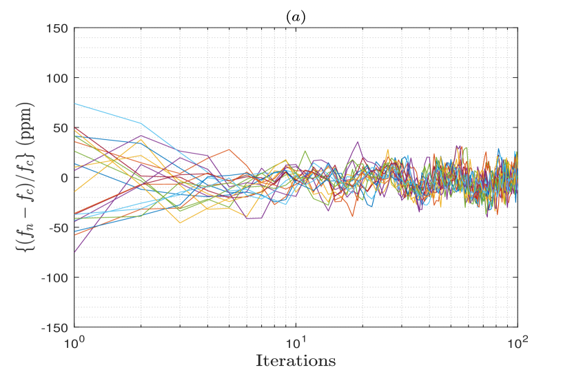
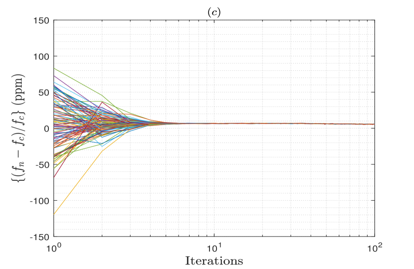
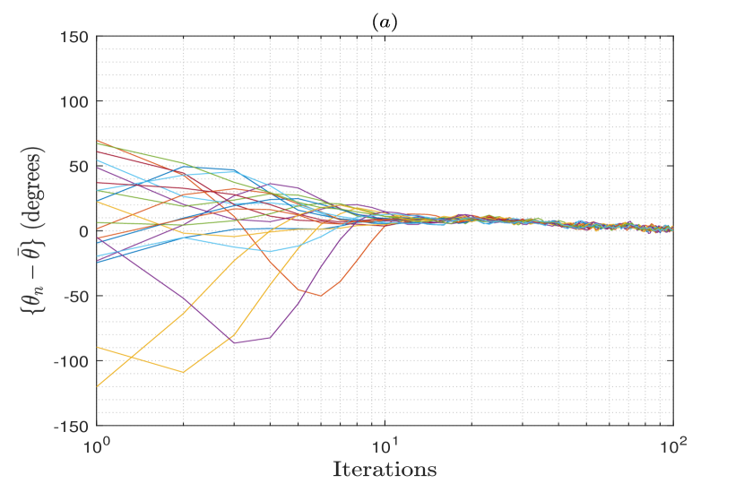
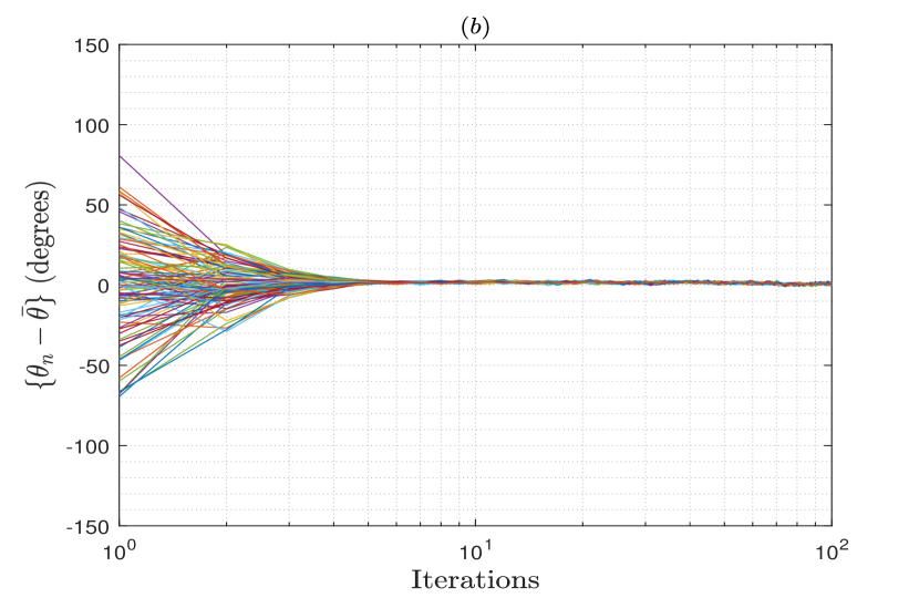
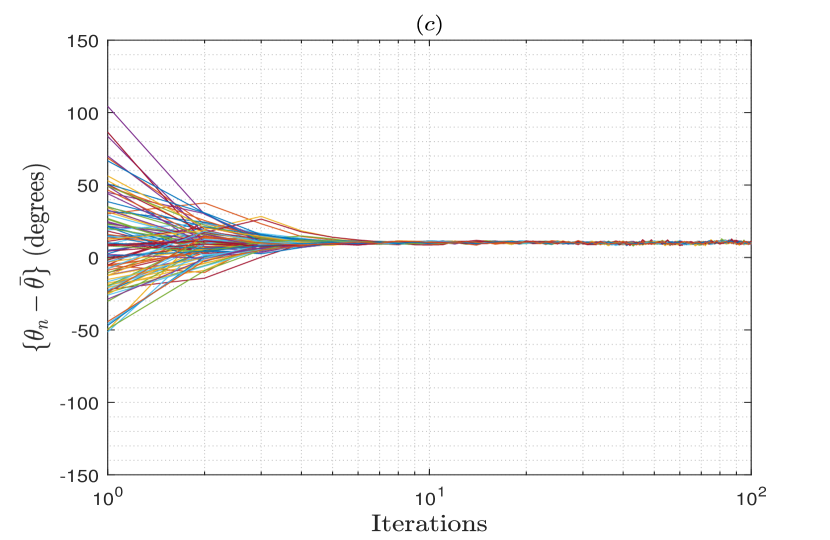
Figs. 1 and 2 show the frequencies and phases for all the nodes in the array relative to their average values vs. the number of iteration of the FPC algorithm from a single trial, when a moderately connected array network with connectivity is generated for the different number of nodes in the array. The SNR of the observed signals is either set as dB or dB. These figures show that with the increase in the number of iterations, both frequencies and phases of the nodes converge to the average of their initial values for all the considered cases. The residual error upon convergence results from the oscillators’ frequency drifts and phase jitters, as well as the frequency and phase estimation errors induced at the nodes. Thus, when the SNR increases to dB for nodes, it is observed that the residual error also decreases significantly upon the convergence due to the decrease in the estimation errors.
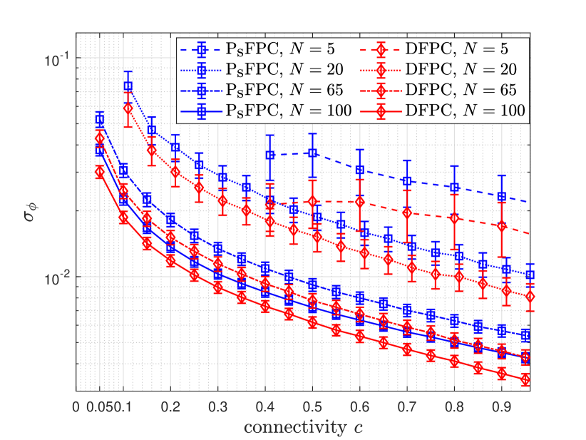
Now let the total residual phase error of node be denoted by . Thus, in Fig. 4, we plot the standard deviation of the total phase errors for all the nodes in the array for the FPC algorithm by varying the connectivity between the nodes and the number of nodes in the array, and when SNR dB is assumed. For the comparison, we generate the bidirectional array networks for each and values and show the standard deviation of the total phase error of the DFPC algorithm proposed in [11] for such array networks. Note that the standard deviation of the DFPC-based algorithms in this work provides the lower bounds on the standard deviation of the total phase error of the FPC-based algorithms, and the slight increase in the phase error of the FPC-based algorithms as compared to the DFPC-based algorithms is due to the decrease in the number of connection per node in the directed networks which effects the accuracy of the local averages computed per node throughout the network as expected. For this figure, both FPC and DFPC algorithms were run for iterations and the final standard deviations of the total phase errors were averaged over trials The center of each point in the error bar plot is the average value of the samples and the length of the bar defines the standard deviation around the average value. It is observed that for each value, as the connectivity between the nodes increases then the total phase error of the FPC and DFPC algorithms decreases proportionately. Furthermore, an increase in the number of nodes in the array, for a given value, also decreases the total phase errors of both algorithms. As discussed in the previous subsection, the decrease in the residual phase error of FPC with the increase in the or values is because the network algebraic connectivity decreases which in turn reduces the residual phase of FPC. The residual phase error of DFPC is also a function of as shown in [11] and thus the same trend is observed for the DFPC algorithm as well.
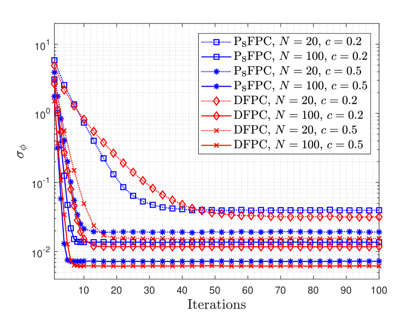
Finally, in Fig. 4, we compare the convergence speeds of the FPC and DFPC algorithms by plotting the standard deviation of the total phase error vs. the number of iteration of the algorithms when the two different and values are assumed and the SNR is set to dB. It is observed that either when increases from to for a given value, or when increases from to for a given value, the FPC algorithm converges faster. Specifically, for and , FPC converges in iterations, but for this value, when increases to , FPC converges in about iterations. Moreover, for and nodes, FPC converges in about iterations. This is because as either or increases then the average number of connections per node in the network, i.e., the value, increases which in turn quickly stabilizes the local averages computed at the nodes. Although the same trend is also observed for the DFPC algorithm in all the considered cases in this figure, particularly it is observed that the FPC algorithm converges faster than the DFPC algorithm in all cases. This is because the network is bidirectional for the DFPC algorithm, and as such there are more connections per node in the network which in turn delays the convergence of the local averages computed at the nodes. Note that the FPC algorithm can be deployed for a bidirectional network as well, in which case it results in the same synchronization and convergence performance as that of the DFPC algorithm; however, the DFPC algorithm does not converge in case of directed networks due to its dependence on the average consensus algorithm [15] as discussed before. In practice, since the failure of a link may not be easily detectable, this means that the FPC algorithm is a preferred choice over the DFPC algorithm.
III Mitigating Residual Phase Errors with Online Expectation-Maximization and Kalman Filtering
In order to reduce the residual phase error of the FPC algorithm, we propose to use Kalman filtering (KF) at the nodes that computes the MMSE estimates of the frequencies and phases in each iteration to mitigate the offset errors. KF is applicable in scenarios where the state transitioning model follows a first-order Markov process, and the observations are a linear function of the unobserved state [34]. KF has been used for the time synchronization between the nodes in [35, 36], and for the frequency and phase synchronizations between the nodes in a distributed antenna arrays in [11]. However, an implicit assumption in using KF with the synchronization algorithms in [35, 36, 11] is that the innovation noise and the measurement noise covariance matrices are known to the Kalman filter. As discussed in Section I, these matrices are usually unknown and must be estimated for the KF algorithm. Thus, in this section, we propose to use an online expectation-maximization (EM) algorithm [28] that iteratively computes the maximum likelihood estimates of these noise matrices for Kalman filtering. The EM algorithm is integrated with the KF and FPC algorithms, and the resulting algorithm is referred to herein as EM-KF-FPC. Note that our proposed EM algorithm iteratively computes the ML estimates in an online fashion wherein the estimates are updated instantaneously as the new measurements are recorded. On the other hand, the EM algorithm of [37] assumes a batch mode technique in which a batch of measurements are recorded a priori, and then the EM algorithm is run iteratively on that set of measurements until its convergence. This batch-mode EM algorithm is not applicable in our considered synchronization problem wherein we want to update the nodes in an online manner to avoid larger oscillators drifts and to simultaneously perform the coherent operation during the synchronized interval. Similarly, a variational Bayes (VB) method based hybrid consensus on measurement and consensus on information (VB-HCMCI) algorithm was also proposed in [38], wherein the unknown noise matrices are estimated in an online manner using VB; however, this VB-based algorithm additionally requires a consensus on measurements and a consensus on the predicted information between the nodes at each time instant to result in an improved performance, and they also need to perform multiple iterations at each time instant for the VB’s convergence which makes them computationally more expensive than EM-KF-FPC. We note that performing multiple iterations at each time instant increases the update interval of the nodes in a practical distributed phased array system which is not favorable to avoid the decoherence between the nodes due to the larger oscillator drifts. Furthermore, these VB-based algorithms are developed for the undirected networks using the average consensus algorithm [15], and thus do not converge for the directed ones.
Now, to develop the EM and KF algorithms, we start with describing the temporal variation of the frequencies and phases of the nodes via a state-space model as follows.
III-A State-Space Model
To write the state-space equation for the -th node, let at the -th time instant its state vector be given by in which and represent its frequency and phase, respectively. Using the frequency drift and phase jitter models as described in Section II, the state-space equation for the -th node is written as
| (10) |
in which the innovation noise vector is defined as , and we assume that is normally distributed with zero mean and the correlation matrix which is given by
| (11) |
Next to write the observation equation, let the frequency and phase estimates of the signal for the -th node be written in the vector form as , then in terms of the estimation errors, this observation vector is defined as
| (12) |
in which the measurement noise vector is given by in which and denote the frequency and phase estimation errors, respectively. We assume that is also normally distributed with zero mean and the correlation matrix which is given by
| (13) |
in which the standard deviations and define the marginal distributions on the frequency and phase estimation errors, respectively.
III-B Kalman Filtering
Kalman filtering is an online estimation algorithm that estimates the state vector of the -th node at the current time instant by using all the observations up to the present time. This process involves sequentially computing the prediction-update step and the time-update step at each time instant. To this end, let the state vector estimate of the -th node at time instant be given by the vector whereas its error covariance matrix is defined by the matrix . As annotated in the subscripts, these parameters in KF are computed by using the observations up to time . Thus, in the prediction-update step at time instant , we use the linear transformation in (10) and predict the new state vector estimate and the corresponding error covariance matrix as follows
| (14) |
In the time-update step, an a priori normal distribution is assumed on the state vector where its mean and covariance are set equal to the predicted estimate vector and the error covariance matrix in (III-B), respectively. This a priori distribution is then used to compute the a posteriori mean and covariance of the state vector given the current observation by using
| (15) |
where the Kalman gain matrix is given by
| (16) |
The mean vector in (15) gives the MMSE estimate of the state vector at time instant and the matrix defines its error covariance matrix. These means and covariances of the state vectors are used in the EM algorithm derived below to compute the maximization step in every iteration.
III-C Online Expectation-Maximization Algorithm
The prediction update and time update steps of KF in (III-B) and (15) assume that the innovation noise covariance matrix and the measurement noise covariance matrix are known a priori. As discussed earlier, these model parameters are unknown in practice and must be estimated for Kalman filtering. Let denote the set of these model parameters, then given all the instantaneous observations of the node up to the present time as denoted by , the marginal log-likelihood of is written as
| (17) |
where the conditional distributions in (III-C) can be easily found from (10) and (12) by shifting the distributions of the noise vectors to the given state vectors. Note that due to the normally distributed conditional distributions and due to the log of the summation in (III-C), the above objective function is a non-concave function of , and directly maximizing it with respect to does not provide a closed-form solution for estimating and . An expectation-maximization (EM) algorithm [39, 28] is an iterative algorithm that often results in the closed-form update equations for the unknown parameters and maximizes the marginal log-likelihood function in every iteration until convergence to its local maximum or saddle point [40]. An EM algorithm starts with an initial estimate of the unknown parameters, thus if is the estimate at its -st iteration, in the -th iteration it computes an expectation step (E-step) and a maximization step (M-step). In the E-step, it computes the expectation of the complete data log-likelihood function using the estimate of from the previous iteration as follows.
| (18) |
where the expectation in (18) is a conditional expectation given the observations and the estimate . In the M-step, it maximizes this objective function with respect to to get its new estimate by solving
| (19) |
The above E-step and M-step are repeated iteratively until the convergence is achieved. The EM algorithm in (18) and (19) describes a batch-mode EM algorithm that is proposed in [39, 37] where first the entire data set up to the time instant is collected, and then the algorithm is run iteratively on this data set until convergence is achieved. This batch-mode EM algorithm is applicable in cases where the cost of collecting the entire data set at once is affordable, whereas in our synchronization task due to the oscillators instantaneous frequency drifts and phase jitters, we aim to instantaneously estimate and update the frequencies and phases of the nodes in every iteration to synchronize these parameters across the array.
To instantaneously estimate from the observed data, an online version of the EM algorithm is proposed in [28, 41] where the E-step in (18) is replaced by a stochastic approximation step in the -th iteration as follows.
| (20) |
where is a smoothing factor, and we define
| (21) |
Note that the iteration index in the E-step in (20) is the same as the time index due to the online nature of the algorithm. Assuming a constant smoothing factor with , where can be optimized on an initial dataset [41], the E-step in (20) can be written in compact form as
| (22) |
| (23) |
In the M-step of the online EM algorithm, we maximize the objective function in (III-C) with respect to as in (19).
Now we describe the computation of the auxiliary function in (III-C) as follows. By using the conditional distributions from (10), (12), and (III-C), this function can be computed as shown in (III-C), in which and are the first and second element of the vector , respectively, and the scalars and define the -th and -th indexed elements of the matrix , respectively. The correlation matrices , , , and the mean vector in (III-C), in iteration , are defined in the following. To begin, the matrix is defined by
| (24) |
where by using the fixed-point Kalman smoothing equations from [34], we get the covariance matrix as
| (25) |
in which
| (26) |
and we get the mean in (III-C) as
| (27) |
Similarly, the correlation matrix in (III-C) is defined as
| (28) |
and the correlation matrix in (III-C) is given by using the Kalman filtering time-update equations as
| (29) |
where and are defined in (15). In fact, note that all the matrices in (III-C)-(III-C) are computed using the KF prediction-update and time-update equations defined in (III-B) and (15) in Section III-B.
Next we compute the M-step of the online EM algorithm in which we maximize the auxiliary function in (III-C) to recursively estimate . To this end, to estimate , we take the partial derivative of with respect to the matrix and set it equal to zero. We get the estimate of in the -th iteration as
| (30) |
where to get the recursive form for updating , we write the numerator in (30) as
| (31) |
thus the update equation for is written as
| (32) |
in which and we set . Similarly the matrix can also be estimated in the M-step through computing the partial derivatives. Since it is a diagonal matrix as shown in (13), it can be easily estimated by recursively estimating its diagonal elements and as follows. To estimate , we compute
| (33) |
where , and to estimate , we use
| (34) |
where we set . Thus, and together define the correlation matrix in the -th iteration.
This completes the derivation of the online EM algorithm. For further detail, the pseudo-code of the resulting algorithm which combines EM, KF, and FPC is given in Algorithm 2.
-
a)
Obtain the observation vector .
-
b)
Compute the prediction update step of KF.
-
i.
Run the prediction update of KF by computing
-
i.
Set
Run the time update step of KF by computing
For each , let ,
III-D Discussions
In this subsection, we begin with describing the initialization of the KF algorithm in each iteration, and then compute the computational complexity of the proposed EM-KF-FPC algorithm. Note that the initialization of the EM algorithm is included in Section III-E where the simulation results are discussed.
-
a)
Initialization: To perform the prediction update step of KF in the iteration of the EM-KF-FPC algorithm, we define the mean vector and the covariance matrix of the -th node as and . Next since the posterior distribution on the state vector of node is a normal distribution and the means undergo a linear transformation in Step (e) of EM-KF-FPC algorithm, we initialize the prediction-update step of KF in the iteration by defining the mean vector from the previous iteration as and the covariance matrix as
(35) where and the components , , and are the -th, -th, and -th elements, respectively, of the covariance matrix computed at node in the -st iteration of KF using (15). Noticeably the proposed EM-KF-FPC algorithm is a distributed algorithm in which the nodes run the EM and KF algorithms on their own observations, in parallel, and then locally share their MMSE estimates and the error covariances with their neighboring nodes to update the electrical states in step across the array. The shared covariances are used to define the priors at each node for Kalman filtering in step .
-
b)
Computational Complexity: For the -th node in the array, the computational complexity of EM-KF-FPC per iteration is dominated by (II-A), (16), and (26). Equation (II-A) is part of the FPC algorithm which has the computational complexity of , where the notation defines the cardinality of the set . Equations (16) and (26) are part of the KF and EM algorithms, respectively, which require inverting and then multiplying the matrices. These two equations have the computational complexity of . Now since the KF and EM step in the synchronization algorithm for each node can be run in parallel, the computational complexity of the overall EM-KF-FPC algorithm is . This shows that for the sparsely connected arrays with , the computational complexity is , whereas for the moderately connected large arrays with , it can be approximated as . Thus, for the moderately connected large arrays, using the EM and KF algorithms result in an improved synchronization performance of FPC without any additional increase in the computational complexity. This result is the same as was observed for the KF-DFPC algorithm in [11] which was proposed for the bidirectional array networks. Furthermore, we also note that the computational complexity of EM-KF-FPC is significantly lower than that of the VB-HCMCI algorithm in [38] which not only does additionally require consensus on measurements and consensus on the predicted information at each node that comes at the cost of increase in the bandwidth requirement between the nodes and the increase in the latency for encoding the information, but they also need to perform multiple iterations at each time instant and at each node for the VB’s convergence, before progressing on to the next time instant .
III-E Simulation Results
In this subsection, we evaluate the frequency and phase synchronization performances of the proposed EM-KF-FPC algorithm by varying the number of nodes in the array and the connectivity between the nodes. To this end, we consider different initialization of the online EM algorithm. For the comparison purposes, we plot the performance of the KF-FPC with known innovation noise and measurement noise covariance matrices and refer to it as the Genie-aided-KF-FPC. In addition, we also show the performance of KF-FPC when these noise covariance matrices are not updated over the iterations and the algorithm uses the initially estimated covariance matrices which is referred to herein as the Naive-KF-FPC algorithm. The carrier frequency of the nodes is chosen as GHz, the sampling frequency is set as MHz, the update interval is ms, the SNR dB. The results in this section were averaged over independent trials.
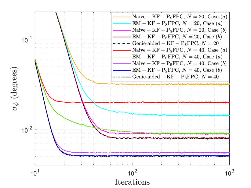
In Fig. 6, we analyze the convergence properties of the EM-KF-FPC algorithm by evaluating the standard deviation of the residual phase error vs. the number of iterations for and nodes in the array with connectivity , and for different initialization of the noise covariance matrices ( and ) in the online EM algorithm. For the demonstration purposes, we consider two cases of the initializations for the EM algorithm in EM-KF-FPC, i.e., case represents a poor initialization of EM with in which , and with , whereas case represents a good initialization of EM with and . Note that the initialization in case uses a poor estimate of that ignores the cross-correlation terms in , uses an estimate of , and assumes that there is no phase jitter at the nodes with . In contrast, the initialization in case uses the true matrix. Furthermore, both cases use a poor estimate of matrix where the true diagonal elements can be computed using the considered simulation parameters in (13) as and . For both of these cases and for both and nodes, we evaluate the residual phase error of EM-KF-FPC vs. the number of iterations and compare it against the Naive-KF-FPC and the Genie-aided-KF-FPC as shown in the figure. It is observed that with the case initialization and for both values, the Naive-KF-FPC algorithm although converges faster but results in a higher residual phase error as compared to EM-KF-FPC. Our EM-KF-FPC algorithm takes about to more iteration to converge when varies from to nodes, respectively, than the Naive-KF-FPC algorithm but significantly reduces the residual phase error upon convergence. Note that, in this case, the residual phase error of EM-KF-FPC is far from the Genie-aided-KF-FPC for both values due to the convergence of EM to the local maximum near the initial estimate as discussed in Section III-C. In contrast, in case , where a better initial estimate is available, the Naive-KF-FPC continues to show a higher residual phase error as compared to EM-KF-FPC, whereas the EM-KF-FPC algorithm follows both the convergence speed and the residual phase error of the Genie-aided-KF-FPC. To summarize, in both cases, EM-KF-FPC performs better than Naive-KF-FPC, and in particular with a good initialization of EM, EM-KF-FPC converges in residual phase error to the Genie-aided-KF-FPC as expected.
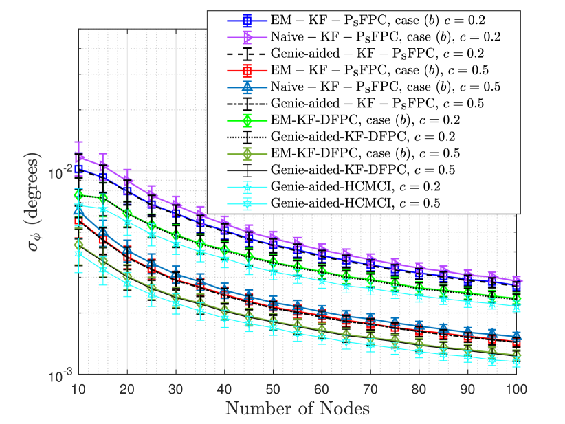
In Fig. 6, we continue with the case initialization and plot the final standard deviations of the residual phase errors of the EM-KF-FPC, Naive-KF-FPC, and Genie-aided-KF-FPC algorithms after iterations by varying the number of nodes in the array and the connectivity between the nodes. It is observed that as the value of or increases, the performance of all the algorithms improves due to the increase in the average number of connections per node () and a decrease in the network algebraic connectivity () as dicussed before. Moreover, by comparing Figs. 4 and 6, it is observed that Kalman filtering significantly reduces the residual phase error of the consensus-based algorithms and thereby minimizes the decoherence between the nodes. For all the and values, the EM-KF-FPC algorithm continues to perform better than the Naive-KF-FPC algorithm and similar to the Genie-aided-KF-FPC algorithm. For this figure, we also extended the KF-DFPC algorithm of [11] to integrate the online EM algorithm with it, and thus evaluated the performance of the EM-KF-DFPC algorithm and the Genie-aided-KF-DFPC algorithms. It is observed that for both and , and all values, EM-KF-DFPC performs similar to Genie-aided-KF-DFPC but better than the EM-KF-FPC algorithm. This is expected because the DFPC-based algorithms were evaluated using undirected array networks which entails more exchange of information between the nodes as compared to the directed networks which were used for the FPC-based algorithms. Note that, as mentioned before, the DFPC-based algorithms are only applicable to the undirected array networks with bidirectional links between the nodes, whereas for the directed array networks, they do not converge due to the use of average consensus [15] as the underlying algorithm. However, our proposed FPC-based algorithms are applicable for the both types of array networks, whereas in the case of undirected networks FPC-based algorithms results in the same synchronization and convergence performance as the DFPC-based algorithms. Thus, the performances of the DFPC-based algorithms in this work can also be interpreted as the performances of the FPC-based algorithms for the undirected array networks to drew a comparison of directed vs. undirected array network.
Finally, Fig. 6 also shows the residual phase error of the HCMCI algorithm of [29] for the undirected array networks with consensus steps, which is the base algorithm of VB-HCMCI (see Table I in [38]). To this end, we assume here that the noise covariance matrices are known to the HCMCI algorithm, and thus refer to it as the Genie-aided-HCMCI algorithm. It is observed that the Genie-aided-HCMCI performs slightly better than the EM-KF-DFPC (EM-KF-FPC) algorithm for all the and values. As discussed earlier, this is because HCMCI-based algorithms additionally need to perform a consensus on the neighboring nodes’ measurements and a consensus on their predicted information matrices in each iteration as compared to the KF-DFPC and KF-FPC based algorithms which only perform consensus on the MMSE estimates and the error covariances at the neighboring nodes. Hence, the latter ones are computationally less complex and have lower latency in encoding the information and the lower bandwidth requirement for sharing that information between the nodes as compared to the HCMCI-based algorithms.
IV Conclusions
We considered the problem of joint frequency and phase synchronization of the nodes in distributed phased arrays. To this end, we included the frequency drift and phase jitter of the oscillator, as well as the frequency and phase estimator errors in our signal model. We considered a more practical case, that is when there exist directed communication links between the nodes in a distributed phased array. A push-sum protocol based frequency and phase consensus algorithm referred to herein as the FPC algorithm was proposed. Kalman filtering was also integrated with FPC to propose the KF-FPC algorithm. KF assumes that the innovation noise and the measurement noise covariance matrices are known which is an impractical assumption. An online EM based algorithm is developed that iteratively computes the ML estimates of these unknown matrices which are then used for KF. The residual phase error of EM upon convergence is defined by the initialization which is expected due to the non-concave structure of the objective function. However, given a good initialization, the proposed EM-KF-FPC algorithm significantly improves the residual phase error as compared to the FPC and the Naive-KF-FPC algorithms, and also shows similar synchronization and convergence performance as that of the Genie-aided-KF-FPC. The residual phase error and the convergence speed of EM-KF-FPC improves by increasing the number of nodes in the array and the connectivity between the nodes. Furthermore, the computational complexity of EM-KF-FPC is lower than that of the HCMCI-based algorithms and is the same as the computational complexity of the KF-FPC and KF-DFPC algorithms. In particular, for the moderately connected large array, the use of EM and KF doesn’t increase the computational complexity of FPC.
References
- [1] S. M. Ellison, S. R. Mghabghab, and J. A. Nanzer, “Multi-Node Open-Loop Distributed Beamforming Based on Scalable, High-Accuracy Ranging,” IEEE Sensors Journal, vol. 22, no. 2, pp. 1629–1637, 2022.
- [2] S. Schieler, C. Schneider, C. Andrich, M. Döbereiner, J. Luo, A. Schwind, P. Wendland, R. S. Thomä, and G. Del Galdo, “OFDM Waveform for Distributed Radar Sensing in Automotive Scenarios,” in 2019 16th European Radar Conference (EuRAD), 2019, pp. 225–228.
- [3] B. Pardhasaradhi and L. R. Cenkeramaddi, “GPS Spoofing Detection and Mitigation for Drones using Distributed Radar Tracking and Fusion,” IEEE Sensors Journal, pp. 1–1, 2022.
- [4] U. Madhow, D. R. Brown, S. Dasgupta, and R. Mudumbai, “Distributed massive MIMO: Algorithms, architectures and concept systems,” in 2014 Information Theory and Applications Workshop (ITA), 2014, pp. 1–7.
- [5] J. A. Nanzer, S. R. Mghabghab, S. M. Ellison, and A. Schlegel, “Distributed Phased Arrays: Challenges and Recent Advances,” IEEE Transactions on Microwave Theory and Techniques, vol. 69, no. 11, pp. 4893–4907, 2021.
- [6] K.-Y. Tu and C.-S. Liao, “Application of ANFIS for Frequency Syntonization Using GPS Carrier-Phase Measurements,” in 2007 IEEE International Frequency Control Symposium Joint with the 21st European Frequency and Time Forum, 2007, pp. 933–936.
- [7] R. Mudumbai, B. Wild, U. Madhow, and K. Ramch, “Distributed beamforming using 1 bit feedback: From concept to realization,” in in Allerton Conference on Communication, Control, and Computing, 2006.
- [8] W. Tushar and D. B. Smith, “Distributed transmit beamforming based on a 3-bit feedback system,” in 2010 IEEE 11th International Workshop on Signal Processing Advances in Wireless Communications (SPAWC), 2010, pp. 1–5.
- [9] B. Peiffer, R. Mudumbai, S. Goguri, A. Kruger, and S. Dasgupta, “Experimental demonstration of retrodirective beamforming from a fully wireless distributed array,” in MILCOM 2016 - 2016 IEEE Military Communications Conference, 2016, pp. 442–447.
- [10] J. A. Nanzer, R. L. Schmid, T. M. Comberiate, and J. E. Hodkin, “Open-Loop Coherent Distributed Arrays,” IEEE Transactions on Microwave Theory and Techniques, vol. 65, no. 5, pp. 1662–1672, 2017.
- [11] M. Rashid and J. A. Nanzer, “Frequency and Phase Synchronization in Distributed Antenna Arrays Based on Consensus Averaging and Kalman Filtering,” arXiv preprint arXiv:2201.08931v2, 2022.
- [12] S. R. Mghabghab and J. A. Nanzer, “Open-Loop Distributed Beamforming Using Wireless Frequency Synchronization,” IEEE Transactions on Microwave Theory and Techniques, vol. 69, no. 1, pp. 896–905, 2021.
- [13] M. Pontón and A. Suárez, “Stability analysis of wireless coupled-oscillator circuits,” in 2017 IEEE MTT-S International Microwave Symposium (IMS), 2017, pp. 83–86.
- [14] M. Pontón, A. Herrera, and A. Suárez, “Wireless-Coupled Oscillator Systems With an Injection-Locking Signal,” IEEE Transactions on Microwave Theory and Techniques, vol. 67, no. 2, pp. 642–658, 2019.
- [15] S. Boyd, P. Diaconis, and L. Xiao, “Fastest Mixing Markov Chain on a Graph,” SIAM Review, vol. 46, no. 4, pp. 667–689, 2004.
- [16] F. S. Cattivelli and A. H. Sayed, “Diffusion LMS Strategies for Distributed Estimation,” IEEE Transactions on Signal Processing, vol. 58, no. 3, pp. 1035–1048, 2010.
- [17] R. Olfati-Saber, “Kalman-Consensus Filter : Optimality, stability, and performance,” in Proceedings of the 48h IEEE Conference on Decision and Control (CDC) held jointly with 2009 28th Chinese Control Conference, 2009, pp. 7036–7042.
- [18] F. S. Cattivelli and A. H. Sayed, “Diffusion Strategies for Distributed Kalman Filtering and Smoothing,” IEEE Transactions on Automatic Control, vol. 55, no. 9, pp. 2069–2084, 2010.
- [19] D.-J. Xin, L.-F. Shi, and X. Yu, “Distributed Kalman Filter With Faulty/Reliable Sensors Based on Wasserstein Average Consensus,” IEEE Transactions on Circuits and Systems II: Express Briefs, vol. 69, no. 4, pp. 2371–2375, 2022.
- [20] F. Walls and J.-J. Gagnepain, “Environmental sensitivities of quartz oscillators,” IEEE Transactions on Ultrasonics, Ferroelectrics, and Frequency Control, vol. 39, no. 2, pp. 241–249, 1992.
- [21] R. Filler and J. Vig, “Long-term aging of oscillators,” IEEE Transactions on Ultrasonics, Ferroelectrics, and Frequency Control, vol. 40, no. 4, pp. 387–394, 1993.
- [22] S.-y. Wang, B. Neubig, J.-h. Wu, T.-f. Ma, J.-k. Du, and J. Wang, “Extension of the frequency aging model of crystal resonators and oscillators by the Arrhenius factor,” in 2016 Symposium on Piezoelectricity, Acoustic Waves, and Device Applications (SPAWDA), 2016, pp. 269–272.
- [23] M. Goryachev, S. Galliou, P. Abbe, and V. Komine, “Oscillator frequency stability improvement by means of negative feedback,” IEEE Transactions on Ultrasonics, Ferroelectrics, and Frequency Control, vol. 58, no. 11, pp. 2297–2304, 2011.
- [24] K. I. Tsianos, S. Lawlor, and M. G. Rabbat, “Push-Sum Distributed Dual Averaging for convex optimization,” in 2012 IEEE 51st IEEE Conference on Decision and Control (CDC), 2012, pp. 5453–5458.
- [25] H. Ouassal, T. Rocco, M. Yan, and J. A. Nanzer, “Decentralized Frequency Synchronization in Distributed Antenna Arrays With Quantized Frequency States and Communications,” IEEE Transactions on Antennas and Propagation, vol. 68, no. 7, pp. 5280–5288, 2020.
- [26] S. R. Mghabghab and J. A. Nanzer, “Impact of VCO and PLL Phase Noise on Distributed Beamforming Arrays With Periodic Synchronization,” IEEE Access, vol. 9, pp. 56 578–56 588, 2021.
- [27] P. Chatterjee and J. A. Nanzer, “A study of coherent gain degradation due to node vibrations in open loop coherent distributed arrays,” in 2017 USNC-URSI Radio Science Meeting (Joint with AP-S Symposium), 2017, pp. 115–116.
- [28] O. Cappe and E. Moulines, “On-line expectation-maximization algorithm for latent data models,” Journal of the Royal Statistical Society: Series B (Statistical Methodology), vol. 71, no. 3, pp. 593–613, 2009.
- [29] G. Battistelli, L. Chisci, G. Mugnai, A. Farina, and A. Graziano, “Consensus-Based Linear and Nonlinear Filtering,” IEEE Transactions on Automatic Control, vol. 60, no. 5, pp. 1410–1415, 2015.
- [30] H. Ouassal, M. Yan, and J. A. Nanzer, “Decentralized Frequency Alignment for Collaborative Beamforming in Distributed Phased Arrays,” IEEE Transactions on Wireless Communications, vol. 20, no. 10, pp. 6269–6281, 2021.
- [31] M. A. Richards, Fundamentals of Radar Signal Processing. McGraw-Hill Professional, 2005.
- [32] P. Rezaienia, B. Gharesifard, T. Linder, and B. Touri, “Push-Sum on Random Graphs: Almost Sure Convergence and Convergence Rate,” IEEE Transactions on Automatic Control, vol. 65, no. 3, pp. 1295–1302, 2020.
- [33] H. Wang, W. Xu, and J. Lu, “Privacy-Preserving Push-sum Average Consensus Algorithm over Directed Graph Via State Decomposition,” in 2021 3rd International Conference on Industrial Artificial Intelligence (IAI), 2021, pp. 1–6.
- [34] S. Sarkka, Bayesian Filtering and Smoothing, ser. Institute of Mathematical Statistics Textbooks. Cambridge University Press, 2013.
- [35] G. Giorgi, “An Event-Based Kalman Filter for Clock Synchronization,” IEEE Transactions on Instrumentation and Measurement, vol. 64, no. 2, pp. 449–457, 2015.
- [36] P. Li, H. Gong, J. Peng, and X. Zhu, “Time Synchronization of White Rabbit Network Based on Kalman Filter,” in 2019 3rd International Conference on Electronic Information Technology and Computer Engineering (EITCE), 2019, pp. 572–576.
- [37] D.-J. Xin and L.-F. Shi, “Kalman Filter for Linear Systems With Unknown Structural Parameters,” IEEE Transactions on Circuits and Systems II: Express Briefs, vol. 69, no. 3, pp. 1852–1856, 2022.
- [38] X. Dong, G. Battistelli, L. Chisci, and Y. Cai, “An Adaptive Consensus Filter for Distributed State Estimation With Unknown Noise Statistics,” IEEE Signal Processing Letters, vol. 28, pp. 1595–1599, 2021.
- [39] A. P. Dempster, N. M. Laird, and D. B. Rubin, “Maximum likelihood from incomplete data via the EM algorithm,” Journal of the Royal Statistical Society, Series B, vol. 39, no. 1, pp. 1–38, 1977.
- [40] C. M. Bishop, Pattern Recognition and Machine Learning (Information Science and Statistics). Secaucus, NJ, USA: Springer-Verlag New York, Inc., 2006.
- [41] B. Schwartz, S. Gannot, and E. A. P. Habets, “Online Speech Dereverberation Using Kalman Filter and EM Algorithm,” IEEE/ACM Transactions on Audio, Speech, and Language Processing, vol. 23, no. 2, pp. 394–406, 2015.