Online Correlation Change Detection for Large-Dimensional Data with An Application to Forecasting of El Niño Events
Abstract
We consider detecting change points in the correlation structure of streaming large-dimensional data with minimum assumptions posed on the underlying data distribution. Depending on the and norms of the squared difference of vectorized pre-change and post-change correlation matrices, detection statistics are constructed for dense and sparse settings, respectively. The proposed detection procedures possess the bless-dimension property, as a novel algorithm for threshold selection is designed based on sign-flip permutation. Theoretical evaluations of the proposed methods are conducted in terms of average run length and expected detection delay. Numerical studies are conducted to examine the finite sample performances of the proposed methods. Our methods are effective because the average detection delays have slopes similar to that of the optimal exact CUSUM test. Moreover, a combined and norm approach is proposed and has expected performance for transitions from sparse to dense settings. Our method is applied to forecast El Niño events and achieves state-of-the-art hit rates greater than 0.86, while false alarm rates are 0. This application illustrates the efficiency and effectiveness of our proposed methodology in detecting fundamental changes with minimal delay.
Keywords: Change point analysis; Correlation structure; El Niño prediction; Knockoff; Sign-flip permutation.
1 Introduction
The detection of abrupt changes in the statistical behavior of streaming data is a classic and fundamental problem in signal processing and statistics (Siegmund, 1985; Poor and Hadjiliadis, 2008; Veeravalli and Banerjee, 2014; Tartakovsky et al., 2014). A change point refers to the time when the underlying data distribution changes, and it may correspond to a triggering event that could have catastrophic consequences if not detected promptly. Therefore, the goal is to detect the change in distribution as quickly as possible, subject to false alarm constraints.
In the multivariate setting where multiple variables are observed, in addition to changes in univariate characteristics, crucial events are often marked by abrupt correlational changes (Cabrieto et al., 2018). Such multivariate settings are common in network data, including social networks (Raginsky et al., 2012; Peel and Clauset, 2015), sensor networks (Raghavan and Veeravalli, 2010), and cyber-physical systems (Nurjahan et al., 2016; Chen et al., 2015; Lakhina et al., 2004). The correlation changes are significant in various real-world applications. For example, in economics, increasing associations among diverse financial assets are often associated with financial crises (Galeano and Wied, 2017; Wied, 2017). In climate science, the El Niño events, the most important phenomenon of contemporary natural climate variability, exemplifies a phenomenon in which interactions between different locations in the Pacific strengthen before and weaken during events (Ludescher et al., 2013). In seismic detection, the correlations between the sensors strengthen when a seismic event occurs (Xie et al., 2019).
Change point detection in correlation structure has been extensively studied in conventional low-dimensional settings, i.e. the dimension remains small, and the sample size can become very large. For example, Wied (2017) constructed a bootstrap variance matrix estimator to detect changes in the correlation matrix, and Cabrieto et al. (2018) proposed a Gaussian kernel-based change point detection method that can locate multiple change points simultaneously. Madrid Padilla et al. (2023) localized multiple change points in multivariate time series with a potentially short-range dependence. Change point detection in time series has also been studied in Killick et al. (2013) and Dette et al. (2019), as well as the references therein. However, in large-dimensional settings where the dimension can be larger than the (available) sample size, methods designed for the low-dimensional settings often perform poorly or are poorly defined. For example, kernel-based methods are sensitive to kernel function and parameter choices, particularly in moderate to large dimensions, and the method proposed by Wied (2017) is unstable when the dimension is large relative to the sample size due to the (near) singularity of the variance estimator.
For large-dimensional data, Choi and Shin (2021) proposed a break test based on the self-normalization method, which avoids variance estimation. Li and Gao (2024) introduced a sign-flip parallel analysis-based detection method and a two-step approach to locate change points. In addition, since the correlation matrix is a particular case of the covariance matrix, some methods designed to detect changes in covariance can be applied to detect changes in correlation. For example, Dette et al. (2022) presented a two-stage bootstrap approach to detect and locate change points in the covariance structure of large-dimensional data. These existing works focus mainly on offline settings, assuming a fixed data sequence of finite length collected before analysis. These methods are not directly applicable in online settings where data arrive in an online manner.
There is a line of work on detecting covariance changes in online settings. Xie et al. (2020) discussed online monitoring of multivariate streaming data for changes in covariance matrices, focusing on a specific covariance structure that transitions from the identity matrix to an unknown spike covariance model. They proposed the largest-eigenvalue Shewhart chart and the subspace cumulative sum detection procedure. Buzun and Avanesov (2018) used the sup norm of a matrix as their statistics and considered abrupt changes in the inverse covariance matrix and the covariance matrix of large-dimensional data, respectively. Their methods used entirely data-driven algorithms with bootstrap calibration to select thresholds, and the temporal independence of random variables was assumed. Li and Li (2023) considered the Frobenius norm and introduced a novel stopping rule that accommodates spatial and temporal dependencies, applicable to non-Gaussian data. However, it is worth mentioning that relying solely on the covariance matrix for analysis may be susceptible to noise interference, making the correlation matrix more reliable for certain applications. This is evidenced by the real data analysis in Li and Gao (2024), which accurately detected changes in the coronary artery disease index in rearranged RNA data using correlation analysis, while covariance-based methods did not.
This paper focuses on online change detection of correlation matrices. We do not restrict a particular parametric form for the distributions, but only assume that the pre- and post-change distributions employ different and unknown correlation matrices. We assume the availability of a reference dataset generated from the pre-change distribution, which is used to estimate the pre-change correlation matrix. The post-change correlation matrix is estimated from the data sequences and compared with the reference to compute detection statistics. Moreover, we incorporate both the and norms to effectively accommodate the sparse and non-sparse changes in the correlation structure.
The main contributions of the paper are threefold. First, our efficient algorithms are the first to detect correlation changes in large-dimensional streaming data. The proposed methods utilize SMOTE and knockoff techniques to enhance sample efficiency. Second, we characterize the theoretical performance of the proposed methods, specifically in terms of the average run time and the expected detection delay. Finally, a major novelty is the application to El Niño forecasting, and early warnings can be used to predict long-term climate states. Using high-quality observational data available since 1950, our method yields hit rates greater than 0.86, whereas false alarm rates are zero. With this perspective, our method enables applications in many other real problems, such as detecting microearthquakes and tremor-like signals in seismic datasets as soon as possible, which are weak signals caused by minor subsurface changes in the Earth.
The paper is organized as follows. Section 2 presents our problem setup and preliminaries. Section 3 introduces the proposed online detection procedure and two improved methods incorporating the synthetic minority oversampling technique (SMOTE) and knockoff techniques. More importantly, a sign-flip permutation method is proposed to select thresholds used in detection procedures. Section 4 presents the theoretical results of the proposed methods in terms of average run length and worst-case average detection delay. Simulations and El Niño forecasting are discussed in Sections 5 and 6, respectively. Section 7 concludes with a brief discussion. Supplementary materials for this article are available online including all the proofs and an application to seismic event detection.
Notation.
We use to denote the probability measure on the sequence of observations when the change never occurs, and is the corresponding expectation. Similarly, denotes the expectation when the actual change point is equal to ; thus refers to the expectation under the post-change regime. The functions and represent the pre- and post-change probability density functions of the observations, respectively. For a vector , denotes its norm, and denotes its norms. For a matrix , is its Frobenius norm. We denote as the -th to -th columns of the matrix . We use and for the standard big-O and little-o notation. Finally, the symbol is the Hadamard (element-wise) product.
2 Problem Setup and Preliminaries
2.1 Problem Setup
Consider a sequence of observations , where . In general, we do not impose any restriction on , except in the knockoff enhancement discussed in Section 3.4. We are interested in detecting the change point in the underlying correlation structure. We assume the following data-generating model:
Here, is the change-point at which the correlation structure of changes. The matrices and are the pre- and post-change correlation matrices, respectively. We assume that both and are unknown, and the change point is deterministic and unknown. The difference between and indicates the magnitude and pattern of the change. Specifically, the correlation change is considered sparse if the number of differing entries between and is relatively small compared to the total number of entries, otherwise the change is considered dense.
Our goal is to detect the change as quickly as possible, subject to false alarm constraints. This is usually achieved by designing a stopping time (Poor and Hadjiliadis, 2008), which is a random variable relating to the data sequence such that for each , the event , where denotes the sigma-algebra generated by . Equivalently, the event is a function of only .
2.2 Performance Measures
A fundamental objective in sequential change point detection is to optimize the trade-off between false alarm rate and average detection delay. Controlling a false alarm rate is commonly achieved by setting an appropriate threshold on a test statistic. On the other hand, the threshold also affects the average detection delay. A larger threshold incurs fewer false alarms but leads to a larger detection delay, and vice versa.
We introduce next the two commonly used performance metrics in sequential detection, the average run length (ARL) and the worst-case average detection delay (WADD). ARL is used to characterize false alarms and it is defined, for a given stopping time , as:
| (1) |
its reciprocal is the commonly used false-alarm rate . ARL can be interpreted as the expected time duration between two consecutive false alarms. We typically focus on the test procedures that satisfy a constraint on the ARL, i.e., consider the set of tests:
notice that ARL (or ) is pre-specified and can go to infinity.
Finding a uniformly powerful test that minimizes the delay over all possible values of the change point , subject to an ARL constraint, is generally intractable. Usually, it is more tractable to pose the problem in the so-called minimax setting. We adopt the worst-case detection delay (WADD), defined as the supremum of the average detection delay conditioned on the worst possible realizations (Lorden, 1971). More specifically,
| (2) |
where is essential supremum, and . Under such a definition of WADD, the formulation of interest is:
| (3) |
Remark 2.1 (Information-theoretic lower bound).
The information-theoretic lower bound to , i.e., the minimum value of (3), is known to be obtained by the CUSUM Procedure (Page, 1954), which is a commonly used sequential change detection procedure that enjoys efficient implementation and exact optimality properties (Lorden, 1971; Moustakides, 1986; Ritov, 1990). By accumulating the log-likelihood ratios, the CUSUM statistic is constructed as , where is the log-likelihood ratio statistic, and the stopping time is thus , for a pre-specified threshold such that . The WADD of the CUSUM test is known to be , where is the KL divergence between the post- and pre-change distributions (Tartakovsky et al., 2014). In Section 5, we compare the performance of the proposed detection methods with that of the CUSUM procedure to validate their effectiveness. It is important to note that the CUSUM test requires full knowledge of the pre- and post-change density functions, which is usually unavailable in practice.
Remark 2.2 (How does influence the detection procedure?).
The dimensionality of the data, , significantly affects the correlation structure before and after a change point, which, in turn, affects the detection delay for a fixed ARL. Higher dimensions can lead to more complex correlations, potentially masking the detection of changes. Generally, as increases, the detection delay may increase due to a diminished signal-to-noise ratio and increased sensitivity to noise. In Section 5, however, our results indicate a shorter detection delay as increases, demonstrating the bless dimension property of our detection method.
3 Online Detection Procedure
In this section, we first introduce the construction of sliding sample correlation matrices and define some preliminary statistics in Section 3.1. We then propose sum-type and max-type detection statistics, together with their window-limited and Shewhart-type variants, in Sections 3.2 and 3.3, respectively. We discuss SMOTE and knockoff enhancements in Section 3.4, providing solutions for situations with limited sample sizes. In addition, we present a practical method for threshold selection in Section 3.5, which ensures computational and sample efficiency while maintaining the desired ARL condition approximately.
3.1 Sliding Sample Correlation Matrices and Preliminary Statistics
Assume a data sequence that is i.i.d., where with bounded fourth-moment entries and correlation matrix . The matrix can be estimated using the sample correlation matrix defined as follows. There are typically two scenarios, depending on the prior knowledge of the distributional parameters. For illustration purposes, we first consider the simplest case where the mean and variance of each entry are known. Without loss of generality, we assume and , . The sample correlation matrix for samples within a time window is then given by .
Second, we consider the general case where the population mean and variance are unknown. Let be the sample mean from time to , and the corresponding sample covariance matrix within is
| (4) |
Let be the diagonal matrix of and be the standardized vector of , for , then the corresponding sample correlation matrix for samples within is
| (5) |
Assume there is also a set of reference data (historical data) of size , which are known to be generated from the pre-change distribution with an unknown correlation matrix . According to equation (5), the sample correlation matrix of all reference data can be similarly calculated as:
| (6) |
where , for , and we further denote . The size of historical data, , is assumed to be sufficiently large. When appropriate, we may use only a subset of this historical data for calculating the sample correlation matrix.
Given the online sequence , we calculate the detection statistics as follows. At each time , we investigate all values of as potential change-points. For each , we calculate the sample correlation matrix according to (5) using potential post-change samples . Then, we calculate the squared difference between and , i.e.,
| (7) |
where indicates the half-vectorized vector by vectorizing only the lower triangular part (excluding the diagonal) of the symmetric matrix. If a change point exists at , then is obviously an estimator of , which measures the entry-wise differences between the pre- and post-change population correlation matrices.
More specifically, for any -th entry of the correlation matrix, we present the expectation of when the data sequence is sampled entirely from the post-change regime, to illustrate its effectiveness for detection. For notational convenience, we write and here.
Lemma 3.1.
Assume and for , , for , we have
| (8) |
where is the expectation under the pre-change regime, and is the expectation under the post-change regime.
We note that in (8), the first term dominates the expectation when and are sufficiently large. Therefore, for any fixed , larger values of indicate a significant difference between and . In contrast, under the pre-change regime, all elements in the are considerably small.
Remark 3.2 (The case with unknown mean).
In the more general case with unknown mean value and known unit variance for , , the expectation of is
The first term is still the dominating term. When the variance is also unknown, the sample variances serve as consistent estimators for and the expectation of can be approximated similarly as above.
Remark 3.3.
Although we assume the data follows an i.i.d. distribution, our proposed method is not restricted to i.i.d. cases. The strong assumptions outlined in Lemma 3.1 and Remark 3.2 are primarily for theoretical analysis. In Section 5 and Section 6, our method demonstrates robust performance in more complex scenarios, including non-Gaussian distributions and serial dependence.
3.2 Sum-Type Detection Statistics
To detect dense changes in correlation structure, we use the norm of to construct detection statistics. Since the true change-point location is unknown, we take the maximum for all potential change-point , and the resulting detection statistic is defined as
| (9) |
the scaling is incorporated to balance the variance of , as the variance of is . When is relatively large, we may simply use .
Window-limited variant
In practice, searching for the maximum over is computationally expensive, especially when becomes larger. Alternatively, we can use the window-limited sum-type statistic (WL-Sum) defined as
| (10) |
where is a pre-specified window size.
Shewhart-type variant
Alternately, we can further improve computational efficiency by eliminating the maximization step on at time . This leads to the following Shewhart sum-type (ST-Sum) statistics:
| (11) |
Change detection is performed by stopping time defined as
where is the pre-specified threshold selected to meet the false alarm rate constraint, as detailed later. Here can be any sum-type test statistic mentioned above, and it is worth noting that the detection threshold varies for different test statistics.
3.3 Max-Type Detection Statistics
The sum-type detection statistics above may not be efficient in detecting sparse changes, where only a relatively small number of elements change in the correlation structure. Under the sparse setting, the conventional test statistic is the maximum difference between the pre- and post-change correlation matrices. We thus define the max-type test statistic as
| (12) |
Window-limited variant
A window-limited variant of the max-type statistic (WL-Max) is employed to mitigate the computational burden,
| (13) |
Shewhart-type variant
The Shewhart max-type statistic (ST-Max) is similarly constructed as
| (14) |
The stopping time is denoted as,
where can be either or .
Remark 3.4 (The choice of window size.).
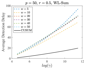
The choice of window size involves a tradeoff between computational efficiency and detection delay. Generally, we assume a small sequence of data is available to pre-determine the optimal window size. A smaller window size may be computationally faster but could result in longer detection delays, especially for large ARL constraints. Conversely, a larger window size improves detection delay but is computationally less efficient. The key idea is to have sufficient data to ensure that the signal-to-noise ratio is detectable. In Proposition 4.3, we provide a lower bound for selecting the window size. A small-scale simulation is conducted to evaluate the impact of the window size , with the results presented in Figure 10 of the Supplementary Material. The key observation is that, for a fixed small ARL value, a wide range of window sizes generally achieves low detection delays, allowing us to select smaller window sizes to ensure computational efficiency. However, as ARL increases, the detection delay for smaller window sizes can grow quadratically, necessitating the use of larger window sizes to maintain detection performance. Additionally, larger window sizes are needed for performing more challenging detection tasks effectively.
Remark 3.5.
An alternative method to improve the computational efficiency of window-limited statistics in (10) and (13) is to use lagged sliding windows with stopping time defined as
where is the lag between neighboring sliding windows, and when , it reduces to the previous definition, and means that we have independent (nonoverlapping) sliding time windows.
3.4 SMOTE and Knockoff Enhancements
For window-limited-variant test statistics, the underlying change point can vary from to , the calculations of and statistics can be unstable due to lack of samples, especially when is small compared to the dimension of data and is close to . To solve this issue, we come up with two modified approaches combining with the SMOTE and Knockoff techniques, respectively. See Figure 1 for an illustration.
SMOTE-based method
The SMOTE technique is an oversampling method designed to deal with imbalanced data in classification problems (Chawla et al., 2002). Specifically, for each sample in the minority class, the nearest five neighbors with the smallest Euclidean distance are identified. One is randomly chosen as , based on which a new SMOTE sample is produced as , where is randomly chosen from a standard uniform distribution on . Blagus and Lusa (2013) investigated SMOTE’s theoretical properties and performance on large-dimensional data.
The proposed methods based on window-limited-variant test statistics can be enhanced by combining SMOTE to effectively detect the change points, and the Algorithm is detailed as follows.
Knockoff-based method
Proposed by Barber and Candès (2015), the knockoff method is designed to select variables that are indeed associated with the response with a controlled false discovery rate (FDR). The knockoff variables imitate the original variables’ correlation structure but have nothing to do with the response. Barber and Candès (2015) achieved exact finite sample FDR control in the homoscedastic Gaussian linear model when (along with a nearly exact extension to the case when ). We enhance our proposed detection procedures by incorporating the knockoff method when .
Specifically, for a matrix , , where and satisfies for all , is a non-negative vector of dimensions , is an orthonormal matrix which is orthogonal to the span of the feature of , and is a Cholesky decomposition, see Barber and Candès (2015) for more details to choose . Then has the same correlation structure as .
The Algorithm is the same as the Algorithm 1, except in the 10th line, , and the 11th line becomes: “For , generate knockoff variables as , and .” Using the knockoff enhancement technique, additional independent random variables are added that maintain the same correlation structure as the original variables. This approach improves the estimation of the correlation matrix, particularly when the sample size is small. Regarding detection delay, for a fixed ARL, this technique would allow us to use a smaller window size for the algorithm to identify change points effectively, as shown in Section 5.

Remark 3.6.
A small simulation study is conducted to show the effects of these two enhancement methods on correlation estimation. Two settings are considered under different ground truth correlation matrices,
-
•
Setting 1: the true correlation matrix is an identity matrix ;
-
•
Setting 2: the true correlation matrix is with for , for , .
Table 1 compares the means and standard deviations of , where is the sample correlation matrix calculated from the original samples (of size ), the SMOTE enhancement samples and the knockoff enhancement samples, respectively. Different combinations of data dimension and sample size are considered. Compared to the sample correlation matrix obtained from the original samples, knockoff method can enhance the accuracy of correlation estimation, while the SMOTE method cannot (but the bias is small). This is due to the construction principle of knockoff variables; they keep the same correlation structure with original ones, while SMOTE method only makes sure new SMOTE variables have the same distribution with the original ones.
| Setting 1 | Setting 2 | ||||||
|---|---|---|---|---|---|---|---|
| Original | SMOTE | Knockoff | Original | SMOTE | Knockoff | ||
| Mean | 11.3541 | 11.9440 | 11.2093 | 8.6080 | 8.9213 | 8.5133 | |
| Std | 0.2215 | 0.2816 | 0.2224 | 1.6088 | 1.4629 | 1.6260 | |
| Mean | 22.8313 | 23.9804 | 22.6955 | 17.1047 | 17.8367 | 17.0168 | |
| Std | 0.2192 | 0.3524 | 0.2207 | 2.8597 | 2.6303 | 2.8764 | |
| Mean | 68.7075 | 72.1942 | 68.5769 | 51.7309 | 53.7253 | 51.6465 | |
| Std | 0.1981 | 0.7886 | 0.1987 | 9.6532 | 8.7277 | 9.6662 | |
| Mean | 42.7811 | 45.7033 | 42.7045 | 32.8976 | 34.6930 | 32.8487 | |
| Std | 0.1407 | 0.4921 | 0.1409 | 6.2258 | 5.2383 | 6.2366 | |
| Mean | 30.0997 | 32.5922 | 30.0469 | 22.5139 | 25.3277 | 22.4771 | |
| Std | 0.1067 | 0.3467 | 0.1067 | 3.3156 | 4.0502 | 3.3196 | |
3.5 Signflip-Based Threshold Selection
Selecting a proper threshold for stopping time is crucial in the sequential change point detection procedure. In general, there are two types of methods for determining the appropriate threshold. One way is to infer an exact threshold based on the distribution of test statistics under the pre-change regime. The other way is to determine the threshold based on the empirical distribution of numerous simulated test statistics, which is more common in practice as it requires little knowledge about the distribution of test statistics.
However, in real-data applications where the number of pre-change samples is limited, or when generating samples is time-consuming, the available data size is small. We propose a new heuristic method for selecting the threshold using a sign-flip permutation method, which works well even for small sample sizes. The method is detailed in Algorithm 2. It is worthwhile mentioning that we assume that the prechange correlation matrix is known or preestimated using available historical data in Algorithm 2 for simplicity. In real applications, may be known in advance based on domain knowledge or estimateable from reference data, as shown in our real data analyses in Section 6.
To illustrate why the threshold selected via Algorithm 2 is valid, we present the following lemma.
Lemma 3.7.
Given a random vector and two independent Rademacher vectors and with i.i.d. Rademacher entries, we have and are uncorrelated as for
Lemma 3.7 demonstrates that for a given vector , the data shuffled through various sign-flip steps using different exhibit weak dependence. Moreover, if the shuffled data follows a Gaussian distribution, it becomes independent. This property ensures that the test statistics computed from sign-flip trials are nearly independent, allowing for appropriate threshold selection. A numerical result supporting this assertion is presented in Remark 3.8.
Remark 3.8.
In addition, we illustrate that the sign-flip permutation in Algorithm 2 does not change the distribution of detection statistic under the pre-change measure through a simulation example. We draw pre-change samples from the standard Gaussian distribution with dimension . We set . We plot the detection statistic calculated from the original data and that of from the sign-flipped data in increasing order in Figure 2, where the WL-Sum in (10) is presented, and it is obvious that the two distributions are almost identical.

Remark 3.9.
Before we conclude this section, we would like to comment on the insights behind the effectiveness of SMOTE- and knockoff-enhanced detection procedures in Section 3.4. In the simulation results in Section 5, both SMOTE and knockoff enhanced methods have smaller detection delays compared to the original WL-Sum procedure. We use a simple simulation study to illustrate the key reasons behind the effectiveness of SMOTE and knockoff. We let the pre-change correlation matrix be , and the post-change correlation matrix has entries for and for . We simulate the data sequences of length under both pre- and post-change regimes separately, and use window size for the window-limited approaches.
For ranging from to (999 time steps in total), the number of times when equals to and , are shown, respectively, in Table 2. Under the pre-change regime, among 999 time indices, both SMOTE and knockoff-enhanced methods show more than 91.9% of the times when , making their estimated results more credible and thus the thresholds obtained more reliable. In contrast, the original method has a relatively low number of instances when . In addition, the knockoff-enhanced method consistently finds the maximum of test statistics at . A similar pattern is also observed under the post-change regime. These results align with the detection delay findings presented in Section 5, where the knockoff-enhancement method exhibits the smallest detection delay, followed by the SMOTE-enhancement method, compared to the detection delay of the original WL-Sum statistics .
| Pre-change | SMOTE | 919 | 73 | 7 | 999 | |
|---|---|---|---|---|---|---|
| Knockoff | 999 | 0 | 0 | 999 | ||
| Original | 362 | 165 | 112 | 964 | ||
| SMOTE | 982 | 16 | 1 | 999 | ||
| Knockoff | 999 | 0 | 0 | 999 | ||
| Original | 914 | 72 | 13 | 999 | ||
| Post-change | SMOTE | 852 | 110 | 30 | 999 | |
| Knockoff | 998 | 1 | 0 | 999 | ||
| Original | 247 | 138 | 94 | 930 | ||
| SMOTE | 894 | 78 | 16 | 999 | ||
| Knockoff | 999 | 0 | 0 | 999 | ||
| Original | 311 | 135 | 111 | 953 |
4 Theoretical Analysis
In this section, we provide the theoretical guarantees for the proposed tests with respect to two key performance measures: the average run length and the expected detection delay. The detailed proofs are deferred to Section C of the Supplementary Material.
4.1 ARL Approximation
For simplicity, we let the size of the reference data equal the chosen window size . Note that we can regard the weight before the test statistic as a constant for a given , and we may unify both sum-type statistics for non-sparse settings and max-type statistics for sparse settings since they are, in essence, the combination of element-wise entries. We first characterize the temporal correlation of the statistics as follows, which will be utilized later for the ARL approximation.
Lemma 4.1 (Temporal correlation of sequential detection statistics).
Suppose all samples are i.i.d. from pre-change distribution with and for , , then the correlation between the detection statistics and is
Here is a small time shift from and can be both sum-type and max-type statistics defined in Section 3.
Based on this temporal correlation, we have the following Theorem characterizing the approximate ARL of the proposed detection procedures. The main idea is to use a linear approximation for the correlation between detection statistics and . Then, the behavior of the detection procedure can be related to a random field. By leveraging the localization theorem (Siegmund et al., 2010), we can obtain an asymptotic approximation for ARL when the threshold is large enough.
Theorem 4.2 (ARL Approximation).
Assume under the pre-change measure we have for , , and under Assumption C.1, C.2, C.3 and C.4 detailed in Appendix C, as threshold , the ARL of the stopping time can be approximated as
| (15) |
where , , , , , and can be the stopping time of both sum-type and max-type statistics. is a special function closely related to the Laplace transform of the overshoot over the boundary of a random walk (Siegmund and Yakir, 2007):
where and are the probability density function and the cumulative density function of the standard Gaussian distribution.
The bounded fourth-moment assumption is needed to ensure that the estimated correlation coefficients are reliable estimators, i.e., converge to in probability. Additionally, the Assumption C.1, C.2, C.3 and C.4 are required to ensure the applicability of the localization theorem. In practice, all assumptions can be easily satisfied by data from some commonly used distributions, such as Gaussian distributions and exponential families.
The main contribution of Theorem 4.2 is to provide a theoretical method to set the threshold that can avoid the Monte Carlo simulation, which could be time-consuming, especially when the desired ARL is large. From Theorem 4.2, we can numerically compute the threshold value by setting the right-hand side of Equation (15) to the desired ARL value. Table 3 shows the high accuracy of this approximation result by comparing the threshold obtained from Equation (15) with that obtained from a simulation study. For a sequence of i.i.d standard normal samples, we conduct 1000 sign-flip trials to find the threshold for different ARL values. The results of WL-Sum, WL-Max, ST-Sum, and ST-Max procedures are presented in Table 3, indicating the approximation is reasonably accurate as the relative error is smaller than 1% for WL-Sum, around 7% to 11% for ST-Sum, around 1% for WL-Max and smaller than 8% for ST-Max. We also note that the magnitude of thresholds varies for different test statistics. For example, the WL-Sum statistic involves the summation of terms and results in consistently higher thresholds than max-type statistics.
| ARL | 5,000 | 10,000 | 20,000 | 30,000 | 40,000 | 50,000 | |
|---|---|---|---|---|---|---|---|
| WL-Sum | Simulated | 1.3271 | 1.3379 | 1.3478 | 1.3530 | 1.3589 | 1.3598 |
| Theoretical | 1.3388 | 1.3499 | 1.3603 | 1.3659 | 1.3698 | 1.3729 | |
| ST-Sum | Simulated | 79.1592 | 79.7146 | 80.3381 | 80.7368 | 81.0911 | 81.3835 |
| Theoretical | 78.2469 | 78.8507 | 79.4074 | 79.7111 | 79.9234 | 80.0864 | |
| WL-Max | Simulated | 17.3070 | 17.9350 | 18.5248 | 18.8585 | 19.0879 | 19.1525 |
| Theoretical | 16.7333 | 17.0234 | 17.2975 | 17.4572 | 17.5667 | 17.6469 | |
| ST-Max | Simulated | 1.0308 | 1.0617 | 1.0999 | 1.1168 | 1.1351 | 1.1412 |
| Theoretical | 0.9561 | 0.9732 | 0.9896 | 0.9988 | 1.0052 | 1.0101 |
4.2 Detection Delay of Max-type and Sum-type Statistics
When a change point exists, the performance of the detection procedure is measured by the detection delay as defined in (2), which can be interpreted as the expected number of post-change samples needed to detect the change. We note that the supremum over all possible change-points in the definition (2) is typically intractable for a general detection procedure. Therefore, we use a simplified definition of the expected detection delay (EDD) as , i.e., the expected stopping time when the change point equals , this is also what is typically simulated in practice. We present the following proposition for the detection delay of the proposed stopping times.
Proposition 4.3 (EDD Approximation).
Assume under the post-change measure we have for , , then the EDD of WL-Sum and WL-Max test statistics can be approximated as follows. As threshold and for window size ,
where and are two notions of signal strength, and note that large indicates the change in the correlation matrix is sparse.
5 Simulation Results
In this section, we conduct extensive simulations to illustrate the performance of the proposed methods. The simulations are conducted across varying dimensions and window sizes . We set , , , and all detection delays are averaged at 1000 replications. We consider two data-generating distributions for the stream : (i) Multivariate normal distribution ; and (ii) Multivariate Student’s distribution, , with degree of freedom 5 and covariance matrix . For each type of distribution, we examine three scenarios: Cases 1 and 2 represent non-sparse settings, while Case 3 represents a sparse setting, and Case 4 is a more general setting. Below denotes the off-diagonal element of the post-change correlation matrices, and is the floor function.
-
•
Case 1: ; for .
-
•
Case 2: ; for and 0 otherwise.
-
•
Case 3: , for and 0 otherwise.
-
•
Case 4: for and 0 otherwise, for and 0 otherwise.
We simulate the expected detection delay by setting the change point , which means that all streaming data is drawn from the post-change distribution. This simplifies the simulation process, as computing the exact WADD, defined in (2), which requires considering all possible change points, is often impractical. Importantly, for some detection procedures, such as the CUSUM test, the worst-case detection delay is often achieved when the change occurs at (Xie et al., 2021). As a result, using closely approximates the worst-case scenario, proving a reliable alternative to evaluate detection performance without significant deviation from WADD.
For clarity purposes, here is the notation for different methods. In addition to WL-Sum and WL-Max defined in Section 3.2 and 3.3, WL-Sum+SMOTE and WL-Sum+Knockoff denote methods that incorporate SMOTE and Knockoff enhancements, respectively. CUSUM represents the method utilizing exact CUSUM, which is the exact optimal detection procedure and thus provides us the information-theoretical lower bound to the delay (Moustakides, 1986). For knockoff-enhanced methods, we need , so detection results will be absent for large window sizes when this condition is violated.
Following the definition of sparse in Feng et al. (2022), we define a term “dense” to represent the extent of the change in the correlation structure. Dense refers to the proportion of changed elements within the entire lower triangular of the correlation matrix, excluding the diagonal elements. Therefore, a smaller dense value suggests a more sparse alteration in the correlation structure and vice versa. In Case 1, the dense level is 1. In Case 2, the dense level is In Case 3, the dense level is . From Case 1 to Case 3, the extent of the change in the correlation structure becomes more and more sparse.


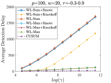


Figure 3 shows the average detection delay (ADD) of different methods under Case 1, with ARL ranging from to . Subfigures (a), (b) and (c) are the results when changes from 0 to 0.3, 0.5 and 0.8, respectively. CUSUM is the optimum detection method that provides the theoretical lower bound on detection delay for all test procedures. For a fixed dense level, when the magnitude of the change in the correlation structure increases, ADD decreases accordingly. Moreover, the SMOTE and knockoff enhanced methods can effectively reduce detection delay, and the knockoff-enhanced method performs better. Comparing (b), (d) and (f), as increases from 50 to 300, the maximum ADD of WL-Sum (WL-Sum+SMOTE, WL-Sum+Knockoff) decreases, indicating that our proposed methods perform better as the dimension grows, that is, blessing of dimension. Comparing (b) and (e), as window size increases from 20 to 50, ADD does not change much for WL-Sum and WL-Sum+SMOTE. Thus, for this setting, the best detection approach is to use a small window size along with knock-off enhancements.
Figure 4 compares the ADDs of different methods in Case 2. Comparing (a) with (b) of Figure 3, as the dense level drops from 1 to 0.2449, the ADD of WL-Sum increases from 47.2 to 75.6, indicating a more challenging detection situation when the change becomes scarce. Moreover, (a) and (b) differ in window size, with little impact on ADD, showing that window size has little influence in this case. But SMOTE can reduce detection delay when is larger. Figures (a), (c), and (d) show that as grows, the ADD decreases, further demonstrating the effectiveness of our proposed method in dealing with large-dimensional data.
Figure 5 compares the ADDs of WL-Sum, WL-Max and their corresponding enhancement methods under Case 3. In all settings, the ADDs of the WL-Sum statistic and its enhancement methods are much larger than the WL-Max type statistics. This indicates that max-type statistics perform better under sparse settings. In addition, the enhancement methods only yield modest improvements to the ADD for WL-Max statistics. Compared with the ADD of the exact CUSUM test, we note that the ADDs of our proposed methods, especially the knockoff-enhanced methods, are comparable to those of exact CUSUM, demonstrating the effectiveness of our methods.
To assess the performance of our method with data generated from the Student’s distribution, the results are presented in Figure 6, which compares the ADDs of WL-Sum and its corresponding enhanced methods under Case 1 and Case 2. Our method demonstrates strong and robust performance under the distribution as well.
Figure 7 compares the ADDs of WL-Sum and its corresponding enhanced methods in Case 4, where is not an identity matrix. Subfigure (a) presents data generated from normal distribution, while subfigure (b) illustrates data from Student’s distribution. For the more general case of a correlation change, our method still performs well; however, the student’s distribution shows a reduced performance due to the increased difficulty in detection.
As shown above, sum-type statistics perform well for dense correlation changes, while max-type statistics excel for sparse changes. Since the dense level is typically unknown in practice, we can utilize both statistics and calibrate them as follows:
and the stopping time is
where and are the estimated thresholds for WL-Sum and WL-Max statistics, respectively, given a fixed . These thresholds are used to calibrate the WL-Sum and WL-Max statistics to the same magnitude. We denote this method as WL-Sum-Max-Combined, as it operates by running both sum-type and max-type detection procedures in parallel and stopping as soon as either one raises an alarm.
The combined is compared with WL-Sum and WL-Max approaches in terms of ADD in Figure 8. For simplicity, we do not present the performance of enhancement methods here. Their performance should be consistent with those shown in Figure 5. Specifically, the enhancement method for WL-Sum will reduce ADD at lower dense levels, whereas for WL-Max, the enhancement method does not result in significant improvements. We fix ARL to in this setting and let , window sizes . For a given positive integer , let for , for and 0 otherwise, and for and 0 otherwise. When , only the correlation coefficient of variable 1 and variable 2 changes, which is extremely sparse. As increases from 2 to 20, the dense level increases from 0.0006 to 0.1073. The correlation coefficients and are selected to ensure the largest eigenvalue of is between and .
The WL-Max statistic performs well when detecting very sparse changes, and as the dense level increases, the WL-Sum statistic performs better. This finding aligns with the literature on two-sample testing, indicating that the max-type statistic demonstrates higher power in sparse settings. In contrast, the sum-type statistic exhibits higher power in non-sparse settings. The yellow line represents the performance of the combined method, and it works consistently well under both sparse and non-sparse settings. It has a lower ADD than WL-Max in sparse cases and nearly the same ADD as WL-Sum in nonsparse cases.


6 El Niño Event Prediction
In this section, we test our proposed method on a real El Niño dataset. To our knowledge, this is the first time a change point detection procedure has been applied to forecasting El Niño events. Our method achieves state-of-the-art hit rates greater than 0.86 with zero false alarm rates.
El Niño episodes are part of the El Niño-Southern Oscillation (ENSO), which is the strongest driver of interannual climate variability and can trigger extreme weather events and disasters in various parts of the world. Early warning signals of El Niño events would be instrumental for avoiding some of the worst damages.
To forecast El Niño events, many state-of-the-art coupled climate models, as well as a variety of statistical approaches, have been suggested; see the review paper Bunde et al. (2024). Although these forecasts are quite successful at shorter lead times (say, 6 months), they have limited anticipation power at longer lead times. In particular, they generally fail to overcome the so-called spring barrier”, that is, in spring, most methods tend to make wrong predictions for El Niño event. Some methods have been constructed to predict El Niño events beyond 9 months in advance (Ludescher et al., 2013). However, it is almost impossible to forecast these events accurately with more than 12 months in advance. Lenssen et al. (2024) found that ENSO is predictable at least two years in advance only when forecasts are made during strong EI Niño events, while forecasts initialized during other states do not have predictive skill over one year. Our method can predict El Niño events more than one year most of the time.
An El Niño episode is featured by rather irregular warm excursions from the long-term mean state. And an El Niño event is said to occur when the ONI index, the 3-month running mean of the anomaly in sea surface temperature averaged in the NINO3.4 region (5oS-N, 170oW-12W), is above for at least five consecutive months. Ludescher et al. (2013) showed that the strengths of the cross-correlations between the El Niño Basin and the surrounding sites tend to strengthen before El Niño episodes and then weaken significantly. Therefore, we concentrate on the changes in the correlations and show that well before an El Niño episode, the correlations tend to increase first and then decrease sharply. We use this robust observation to forecast El Niño development in advance. The sum-type test statistic is applied here.
We use the 1000hPa temperature weekly data obtained from the ERA5 database at time 00:00 on the 7th, 14th, 21st, and 28th days of each month with a grid size of , spanning from 1974 to 2023. We select the same 207 nodes as Ludescher et al. (2013)(30oS-30oN, 120oE-75oW) containing the El Niño Basin, where the nodes are arranged as a matrix. The data dimension is thus , and is the length of the time series. Reference data is chosen from Jan 7th to Dec 28th, 1971, and Jan 7th to Dec 28th, 1974, as no El Niño event happened during these periods. The window size is set as (a year). As the correlation change only occurs in a subset of 207 nodes, we select nodes that are geographically close to each other as a subset, thus there are 32 subsets as in panel (a) of Figure 9. The ST-Sum statistic (11) is calculated for each specific subset, and the maximum value over the 32 subsets is used as the final detection statistic. The prediction result is shown in panel (b) of Figure 9.
The blue line represents the test statistic, and the yellow and green vertical lines mark the beginning and end of 15 El Niño events from 1974 to 2023. The horizontal green line is the threshold. An alarm indicating the arrival of an El Niño event is triggered every time the test statistics cross the threshold from the top. The alarm results in a correct prediction if, in the following one or two years, El Niño episode sets in; otherwise, it is considered a false alarm. The correct predictions are marked with red arrows. During our detection period from 1974 to 2023, there were 15 years with an El Niño episode (i.e., there were 15 events) and 35 years without one (35 free-events years). Our method yields 16 signals, which correctly predict 13 El Niño events with 0 false alarms, resulting in a hit rate of and a false alarm rate of , as shown in the first column of Table 4. It is worth mentioning that since the statistics may contain some noise, any rise above the threshold by a very small margin (less than 10 in this case) is considered noise and not treated as a real alarm. Such instances are indicated with black dotted lines.


In general, the El Niño events and La Niña events appear in return; that is, an El Niño event is often followed by a La Niña event and and vice versa. However, this is not always the case. Sometimes, several El Niño events occur consecutively without an intervening of La Niña event, and similarly, La Niña events can sometimes appear in succession. Of our 13 predictions, 10 prediction signals that occur during or at the end of a La Niña event, indicating that the El Niño would occur in the next one to two years. The other three prediction signals (in 1977, 1981, and 2002) appear during or at the end of El Niño event, indicating that La Niña will not happen, but another El Niño event will continue to occur. Furthermore, for the strongest El Niño event starting from winter 2014 and ending before summer 2016 with the highest strength (peak) ever recorded, our method gives the first signal in winter 2012, then another signal in summer 2013 and a third signal before the starting point of this event. These three signals not only forecast the existence of El Niño phenomenon in the following two years separately, but also indicate an extreme event together.
Ludescher et al. (2013) forecasted El Niño events with a hit rate of 0.7 and a false alarm rate of 0.1 in the training data (1951-1980), and a hit rate of 0.667 and a false alarm rate of 0.048 in the testing data (1981-2011) when the threshold is set at 2.82, as shown in Figure 2 of their paper. For the same period of test data, the comparison results are presented in the last two columns of Table 4, and the prediction results of our method are detailed in Figure 11 of the Supplementary Material. Our method exhibits superior performance compared to Ludescher et al. (2013)’s method, with two more correct predictions, which increases the hit rate by 0.222. Ludescher et al. (2013)’s method failed to detect the three most recent El Niño events, dating back to 2011. In addition, their method contains two steps - an optimum prediction algorithm is first learned from the training data and then applied to the testing data. Meanwhile, their method can produce different results based on different thresholds. In contrast, our method is easily implemented without optimizing in a training dataset, the threshold is determined by the proposed algorithm, and theoretical guarantees are provided.
| Our method | Our method | Ludescher’s | |
|---|---|---|---|
| Period | 1974-2023 | 1981-2011 | 1981-2011 |
| Hit Rate | 0.867(13/15) | 0.889(8/9) | 0.667(6/9) |
| False Alarm Rate | 0(0/35) | 0(0/21) | 0.048(1/21) |
7 Discussions and Conclusion
In this paper, we propose an online change point detection procedure for correlation structures. Both sum- and max-type statistics are proposed for non-sparse and sparse settings, respectively. These two types of statistics can also be combined in practice, providing more flexibility and efficiency for detection tasks. Simulation studies illustrate the performance of the combined method when the change in correlation structure varies from sparse to dense regimes. In addition, we propose to combine SMOTE and Knockoff techniques to increase sample efficiency, and the enhanced detection procedures have shown smaller detection delays in most simulation scenarios. Furthermore, an efficient sign-flip algorithm is proposed to select the threshold for our detection statistics. Theoretical approximations are also provided for ARL and EDD of detection procedures. More importantly, the proposed detection procedure is applied to forecast El Niño events. Our method can predict these events with one or two years in advance and achieves state-of-the-art hit rates above 0.86 and zero false alarm rates. There is immense societal benefit from these high-accuracy multi-year forecasts, as many human systems make decisions on this timescale.
Given the superior performance in forecasting El Niño events, we believe that our methods can be applied to predict other important climate phenomena, especially those involving varying relationships between different regions of the Earth. The application of our proposed algorithm to forecasting La Niña events will be reported in our future work.
There are several possible extensions of our methods. A direct extension is to detect change points in the covariance structure of streaming large-dimensional data, including general covariance structure changes and special covariance structure changes. In addition, while we constructed the detection statistics based on and norms of the difference between two vectorized correlation matrices, other norms can be used to adapt to different circumstances.
References
- Barber and Candès (2015) R. F. Barber and E. J. Candès. Controlling the false discovery rate via knockoffs. The Annals of Statistics, 43(5):2055–2085, 2015.
- Blagus and Lusa (2013) R. Blagus and L. Lusa. SMOTE for high-dimensional class-imbalanced data. BMC Bioinformatics, 14(1):1–16, 2013.
- Bunde et al. (2024) Armin Bunde, Josef Ludescher, and Hans Joachim Schellnhuber. Evaluation of the real-time El Niño forecasts by the climate network approach between 2011 and present. Theoretical and Applied Climatology, pages 1–10, 2024.
- Buzun and Avanesov (2018) N. Buzun and V. Avanesov. Change-point detection in high-dimensional covariance structure. Electronic Journal of Statistics, 12(2):3254–3294, 2018.
- Cabrieto et al. (2018) J. Cabrieto, F. Tuerlinckx, P. Kuppens, F.H. Wilhelm, M. Liedlgruber, and E. Ceulemans. Capturing correlation changes by applying kernel change point detection on the running correlations. Information Sciences, 447:117–139, 2018.
- Cao et al. (2018) Y. Cao, Y. Xie, and N. Gebraeel. Multi-sensor slope change detection. Annals of Operations Research, 263:163–189, 2018.
- Chawla et al. (2002) N. V. Chawla, K. W. Bowyer, L. O. Hall, and W.P. Kegelmeyer. SMOTE: synthetic minority over-sampling technique. Journal of Artificial Intelligence Research, 16:321–357, 2002.
- Chen et al. (2015) Y. Chen, T. Banerjee, A.D. Dominguez-Garcia, and V.V Veeravalli. Quickest line outage detection and identification. IEEE Transactions on Power Systems, 31(1):749–758, 2015.
- Choi and Shin (2021) J. E. Choi and D. W. Shin. A self-normalization break test for correlation matrix. Statistical Papers, 62(5):2333–2353, 2021.
- Dette et al. (2019) H. Dette, W. Wu, and Z. Zhou. Change point analysis of correlation in non-stationary time series. Statistica Sinica, 29(2):611–643, 2019.
- Dette et al. (2022) H. Dette, G. Pan, and Q. Yang. Estimating a change point in a sequence of very high-dimensional covariance matrices. Journal of the American Statistical Association, 117(537):444–454, 2022.
- Feng et al. (2022) L. Feng, T. Jiang, B. Liu, and W. Xiong. Max-sum tests for cross-sectional independence of high-dimensional panel data. The Annals of Statistics, 50(2):1124–1143, 2022.
- Galeano and Wied (2017) P. Galeano and D. Wied. Dating multiple change points in the correlation matrix. Test, 26(2):331–352, 2017.
- Killick et al. (2013) R. Killick, I. A. Eckley, and P. Jonathan. A wavelet-based approach for detecting changes in second order structure within nonstationary time series. Electronic Journal of Statistics, 7:1167–1183, 2013.
- Lakhina et al. (2004) A. Lakhina, M. Crovella, and C. Diot. Diagnosing network-wide traffic anomalies. ACM SIGCOMM Computer Communication Review, 34(4):219–230, 2004.
- Lenssen et al. (2024) N. Lenssen, P. DiNezio, L. Goddard, C. Deser, Y. Kushnir, S. Mason, M. Newman, and Y. Okumura. Strong El Niño events lead to robust multi-year ENSO predictability. Geophysical Research Letters, 51(12):e2023GL106988, 2024.
- Li and Li (2023) L. Li and J. Li. Online change-point detection in high-dimensional covariance structure with application to dynamic networks. Journal of Machine Learning Research, 24(51):1–44, 2023.
- Li et al. (2015) S. Li, Y. Xie, H. Dai, and L. Song. M-statistic for kernel change-point detection. Advances in Neural Information Processing Systems, 28, 2015.
- Li and Gao (2024) Z. Li and J. Gao. Efficient change point detection and estimation in high-dimensional correlation matrices. Electronic Journal of Statistics, 18(1):942–979, 2024.
- Lorden (1971) G. Lorden. Procedures for reacting to a change in distribution. Annals of Mathematical Statistics, 42(6):1897–1908, 1971.
- Ludescher et al. (2013) J. Ludescher, A. Gozolchiani, M.I. Bogachev, A. Bunde, S. Havlin, and H.J. Schellnhuber. Improved El Niño forecasting by cooperativity detection. Proceedings of the National Academy of Sciences, 110(29):11742–11745, 2013.
- Madrid Padilla et al. (2023) C. M. Madrid Padilla, H. Xu, D. Wang, O. H. Madrid Padilla, and Y. Yu. Change point detection and inference in multivariate non-parametric models under mixing conditions. Advances in Neural Information Processing Systems, 36:21081–21134, 2023.
- Moustakides (1986) G.V. Moustakides. Optimal stopping times for detecting changes in distributions. The Annals of Statistics, 14(4):1379–1387, 1986.
- Nurjahan et al. (2016) N. Nurjahan, F. Nizam, S. Chaki, S. A. Mamun, and M. S. Kaiser. Attack detection and prevention in the cyber physical system. In 2016 International Conference on Computer Communication and Informatics (ICCCI), pages 1–6. IEEE, 2016.
- Page (1954) E. S. Page. Continuous inspection schemes. Biometrika, 41(1/2):100–115, 1954.
- Peel and Clauset (2015) L. Peel and A. Clauset. Detecting change points in the large-scale structure of evolving networks. In Proceedings of the AAAI Conference on Artificial Intelligence, volume 29, pages 2914–2920, 2015.
- Pollak and Yakir (1998) M. Pollak and B. Yakir. A new representation for a renewal-theoretic constant appearing in asymptotic approximations of large deviations. The Annals of Applied Probability, 8(3):749–774, 1998.
- Poor and Hadjiliadis (2008) H. V. Poor and O. Hadjiliadis. Quickest Detection. Cambridge University Press, 2008.
- Raghavan and Veeravalli (2010) V. Raghavan and V.V. Veeravalli. Quickest change detection of a Markov process across a sensor array. IEEE Transactions on Information Theory, 56(4):1961–1981, 2010.
- Raginsky et al. (2012) M. Raginsky, R. Willett, C. Horn, J. Silva, and R. Marcia. Sequential anomaly detection in the presence of noise and limited feedback. IEEE Transactions on Information Theory, 58(8):5544–5562, 2012.
- Ritov (1990) Y. Ritov. Decision theoretic optimality of the CUSUM procedure. The Annals of Statistics, 18(3):1464–1469, 1990.
- Siegmund (1985) D. Siegmund. Sequential Analysis: Tests and Confidence Intervals. Springer, 1985.
- Siegmund and Venkatraman (1995) D. Siegmund and E. S. Venkatraman. Using the generalized likelihood ratio statistic for sequential detection of a change-point. The Annals of Statistics, 23(1):255–271, 1995.
- Siegmund and Yakir (2000) D. Siegmund and B. Yakir. Tail probabilities for the null distribution of scanning statistics. Bernoulli, 6(2):191–213, 2000.
- Siegmund and Yakir (2007) D. Siegmund and B. Yakir. The Statistics of Gene Mapping, volume 1. Springer, 2007.
- Siegmund and Yakir (2008) D. Siegmund and B. Yakir. Detecting the emergence of a signal in a noisy image. Statistics and Its Interface, 1(1):3–12, 2008.
- Siegmund et al. (2010) D. Siegmund, B. Yakir, and N. Zhang. Tail approximations for maxima of random fields by likelihood ratio transformations. Sequential Analysis, 29(3):245–262, 2010.
- Tartakovsky et al. (2014) A. Tartakovsky, I. Nikiforov, and M. Basseville. Sequential Analysis: Hypothesis Testing and Changepoint Detection. CRC press, 2014.
- Veeravalli and Banerjee (2014) V. V. Veeravalli and T. Banerjee. Quickest change detection. In Academic Press Library in Signal Processing, volume 3, pages 209–255. Elsevier, 2014.
- Wied (2017) D. Wied. A nonparametric test for a constant correlation matrix. Econometric Reviews, 36(10):1157–1172, 2017.
- Xie et al. (2019) L. Xie, Y. Xie, and G. V. Moustakides. Asynchronous multi-sensor change-point detection for seismic tremors. In 2019 IEEE International Symposium on Information Theory (ISIT), pages 2199–2203, 2019.
- Xie et al. (2020) L. Xie, Y. Xie, and G. V. Moustakides. Sequential subspace change point detection. Sequential Analysis, 39(3):307–335, 2020.
- Xie et al. (2021) L. Xie, S. Zou, Y. Xie, and V. V. Veeravalli. Sequential (quickest) change detection: Classical results and new directions. IEEE Journal on Selected Areas in Information Theory, 2(2):494–514, 2021.
- Xie and Siegmund (2013) Y. Xie and D. Siegmund. Sequential multi-sensor change-point detection. The Annals of Statistics, 41(2):670–692, 2013.
Appendix A Additional Numerical Results
A small simulation is conducted to illustrate the impact of different window sizes and the results are shown in Figure 10. We let varies from 5 to 50, and CUSUM again serves as the theoretical lower bound for detection delay. The first two rows represent data generated from the Case 1 setting defined in Section 5, while the last two rows correspond to Case 2. For a fixed small ARL, all window sizes exhibit low detection delays, with smaller delays preferred for computational efficiency. However, as ARL increases, the detection delay for smaller window sizes can grow quadratically, necessitating the use of larger window sizes. Comparing the first two rows with the last two, it is evident that a larger window size is required for the more challenging detection scenario in Case 2.


Appendix B Seismic Event Detection
We also implement our proposed approaches in a real seismic dataset collected at Parkfield, California, from 2 a.m. to 4 a.m. on Dec 23rd, 2004. The raw data contains records at 13 seismic sensors that simultaneously record a continuous data stream with a frequency of 250HZ, see Figure 12(a). The goal is to detect micro-earthquakes and tremor-like signals as soon as possible, which are weak signals caused by minor subsurface changes in the Earth. The tremor signal is propagated to each sensor from the source, and the affected sensors observe a similar waveform corrupted by noise. These tremor signals are helpful for geophysical study and predicting potential earthquakes.
To improve computational efficiency, we first perform a down-sampling procedure to reduce the data length to . The first 590 observations do not contain tremor signals and are thus selected as reference data. We use a sliding window of length 200s, i.e., at each time point, we utilize the previous 200 observations to estimate the corresponding correlation matrices as . We use the ST-Sum test statistic in (11) and its trajectory is shown in Figure 12(b). We use 50 signflip trials to get the detection threshold. In practice, we inflate the threshold chosen by the algorithm slightly to ensure a zero-false-alarm rate in the reference data.
In Figure 13, the vertical solid line denotes true event time and the dashed line represents the detected change point. Our proposed method finds three main events at 604, 2093, and 6370 seconds as shown in Figure 13(a), (b), (d), respectively. They match well with the true event catalog, 594, 2090, and 6369 seconds, obtained from the Northern California Earthquake Data Center. We also compare our results with those obtained in Xie et al. (2020) using the same dataset. In Xie et al. (2020), three main events are detected at 615, 2127, and 6371 seconds, corresponding to three actual events at 594, 2124, and 6369 seconds. Both our method and the method in Xie et al. (2020) detect the same first and third events, and for the second event, the one that happened at 2090s has a magnitude of 1.66 while the one that happened at 2124s has a magnitude of 1.1, and they are very close to each other. Compared to Xie et al. (2020), our method has a smaller detection delay in the first event and a comparable delay for the latter two events. Our method also detects the tremor-like signals at 4504s, which corresponds to an actual event at 4475 seconds with a magnitude of 1.58, with a time delay of 29 seconds, see Figure 13(c), while the subspace method in Xie et al. (2020) fails to detect this event. It is worth noting that the change in Figure 13(c) is challenging to detect since the data variation between 2000 and 4000 seconds is very large.


Appendix C Proofs
Proof of Lemma 3.1.
For , we have
Under the assumption that and for , we have , , then we take expectation for every term,
finally, we have,
∎
Proof of Remark 3.2.
Notice that, under the assumption that , we have for and for . Due to the unbiasedness of the sample covariance, we have and .
We first write
We have . For the term (the term can be calculated similarly), we can assume for simplicity under both pre- and post-change regimes.
Note that
For the first term, we have
Note that and (after assuming is zero-mean and unit-variance). We define the following notations:
It is obvious that is decomposed into a summation from to , that is, , then if we take expectation of each term, the summation will be . The detailed expectations for each term are as follows.
Then we calculate the expectation of as
Similarly, for the second term , notice that for any , we can decompose it into the summation of several separate terms, the details are as follows.
The expectation of can be calculated in similar way,
Based on the expectations of and , we have,
Similarly, we can obtain,
Finally, we have,
∎
Proof of lemma 3.7.
Given a vector and two independent Rademacher vectors and with i.i.d. Rademacher entries, then and are sub-gaussian random vectors. due to the property of Rademacher entries. Let , then for , the element in the covariance matrix of is
Then and are asymptotically independent. ∎
Proof of Lemma 4.1.
In this lemma, we calculate the temporal correlation of and , where can represent both sum-type and max-type test statistics. We may unify both sum-type statistics for non-sparse settings and max-type statistics for sparse settings, since they are, in essence, the combination of element-wise entries, with each entry being for a constant . equals 1 for max-type statistics and smaller than for sum-type statistics, depending on the change numbers. Besides, for window-limited variant test statistics, the weight can also be treated as a constant, which does not influence the correlation value. Then the correlation between and is in essence the correlation between and . We give the concrete form of the correlation coefficient as
Then we calculate the covariance and variance terms separately, for the covariance term, we have
For simplicity, we denote , , , then
For the variance term, since due to the independent assumption, we only calculate the first one.
Let , , , , then we take expectation for each term as follows.
Since the correlation is represented as follows,
the numerator equals
and the denominator takes value
Combining these results yields the correlation result
and complete the proof. ∎
Proof of Theorem 4.2.
The proof is based on a general method for computing first passage probabilities first introduced in Pollak and Yakir (1998) and further developed in Siegmund and Yakir (2000) and Siegmund et al. (2010), and commonly used in similar problems (Xie and Siegmund, 2013), Li et al. (2015), Cao et al. (2018). First of all, it is worth mentioning that the probability measure in the following proof always stands for the nominal case where all samples are from the same distribution . For the test statistic defined in this paper
if we suppose , and reaches its maximum value when (as shown in Table 2, this is the most common case), then
let From the existing calculation, we have
Here we denote the moment generating function as
and select by solving the equation . Since is defined by a function of independent random samples, converges to a limit as and converges to a limiting value, denoted by . The transformed distribution for all sequences before position and window size is denoted by
Let
Denote be the set of all possible windows in the scan. Let be the event of interests (the event {}), i.e., the detection procedure stop before time m.
By measure transformation, we have
| (16) | ||||
where
Consider a sequence of fields , let and be approximations of and , respectively, which are measurable with respect to . Given , we assume that for all large ,
Assumption C.1.
and satisfy with probability 1.
Assumption C.2.
There exist and measurable with respect to such that and , with probability at least .
Assumption C.3.
converges to a finite and positive limit denoted by .
Assumption C.4.
There exist and such that for every and for all large enough the probability of the event
is bounded from below by .
Since are fixed in much of the following analysis, we suppress the dependence of the notation on and simply write . Under Assumptions C.1, C.2, C.3 and C.4, a localization lemma allows us to simplify the expectation
into a simpler form
where stands for the variance of under measure . The reduction relies on the fact that for large , the local processes and are approximately independent of the global process . Such independence allows the above decomposition into the expectation of times the expectation involving , treating essentially as a constant.
We first consider the process and and derive the expectation following Siegmund and Yakir (2000).
The covariance between the two terms is given by
When is large, we have that the correlation depends on the difference in a linear form, which shows that we have the random walk in the change time , and the variance of the increment equals to . Following Siegmund and Yakir (2000), we have
Moreover, the process is zero-mean and has variance under the measure . Substituting the result for the expectations in (16) yields
In the limiting case, can be well approximated using Gaussian distribution . The moment generating function then becomes , and the limiting , as the solution to . Furthermore, the summation term can be approximated by an integral, to obtain
| (17) | ||||
Here it is assumed that is large, but small enough that the right-hand side of (17) converges to 0 when . Changing variables in the integrand, we can rewrite this approximation as
| (18) |
From the arguments in Siegmund and Venkatraman (1995), Siegmund and Yakir (2008), we know that is asymptotically exponentially distributed and is uniformly integrable. Hence if denotes the factor multiplying on the right-hand side of (18), then for large , in the range where is bounded away from 0 and , . Consequently, , thereby we complete the proof. Here we omit some technical details needed to make the derivation rigorous. Those details have been described and proved in Siegmund et al. (2010). ∎
Proof of Proposition 4.3.
For and a given detection threshold , when the window size is sufficiently large, at the time of detection (the stopping time ) we have
On the other hand, we have , where is also called the overshoot of the detection procedure and it is of order as (Siegmund, 1985). This yields the first-order approximation for the expected stopping time:
where when is the sum-type detection statistics, and for the max-type detection statistics.
∎