Online conformal prediction with decaying step sizes
3Massachusetts Institute of Technology
[email protected], [email protected], [email protected]
)
Abstract
We introduce a method for online conformal prediction with decaying step sizes. Like previous methods, ours possesses a retrospective guarantee of coverage for arbitrary sequences. However, unlike previous methods, we can simultaneously estimate a population quantile when it exists. Our theory and experiments indicate substantially improved practical properties: in particular, when the distribution is stable, the coverage is close to the desired level for every time point, not just on average over the observed sequence.
1 Introduction
We study the problem of online uncertainty quantification, such as that encountered in time-series forecasting. Our goal is to produce a prediction set at each time, based on all previous information, that contain the true label with a specified coverage probability. Such prediction sets are useful to the point of being requirements in many sequential problems, including medicine (Robinson, 1978), robotics (Lindemann et al., 2023), finance (Mykland, 2003), and epidemiology (Cramer et al., 2022). Given this broad utility, it comes as no surprise that prediction sets have been studied for approximately one hundred years (and possibly more; see Section 1.1 of Tian et al. (2022)).
Formally, consider a sequence of data points , for . At each time , we observe and seek to cover with a set , which depends on a base model trained on all past data (as well as the current feature ). After predicting, we observe , and the next time-step ensues. Note that we have not made any assumptions yet about the data points and their dependencies.
This paper introduces a method for constructing the prediction sets that has simultaneous best-case and worst-case guarantees—that is, a “best of both worlds” property. We will describe the method shortly in Section 1.1. Broadly speaking, the method can gracefully handle both arbitrary adversarial sequences data points and also independent and identically distributed (I.I.D.) sequences. In the former case, our method will remain robust, ensuring that the historical fraction of miscovered labels converges to the desired error rate, . In the latter case, our method will converge, eventually producing the optimal prediction sets. We summarize our results below:
-
1.
Worst-case guarantee (Theorem 1): When the data points are arbitrary, our algorithm achieves
(1) for a constant and any fixed . We call this a long-run coverage guarantee.
-
2.
Best-case guarantee (Theorem 3): When the data points are I.I.D., our algorithm achieves
(2) We call this a convergence guarantee.
Our algorithm is the first to satisfy both guarantees simultaneously. Moreover, the decaying step size yields more stable behavior than prior methods, as we will see in experiments. See Section 1.2 for a discussion of the relationship with other methods, such as those of Gibbs and Candes (2021), Angelopoulos et al. (2023), and Xu and Xie (2021).
1.1 Method and Setup
We now describe our prediction set construction. Borrowing from conformal prediction, consider a bounded conformal score function , at each time . This score is large when the predictions of the base model disagree greatly with the observed label; an example would be the residual score, , for a model trained online. This concept is standard in conformal prediction (Vovk et al., 2005), and we refer the reader to Angelopoulos and Bates (2023) for a recent overview. Given this score function, define
| (3) |
where the threshold is updated with the rule
| (4) |
In particular, if we fail to cover at time , then the threshold increases to make the procedure slightly more conservative at the next time step (and vice versa).
Familiar readers will notice the similarity of the update step (4) to that of Gibbs and Candes (2021); Bhatnagar et al. (2023); Feldman et al. (2023); Angelopoulos et al. (2023), the main difference being that here, can change over time—later on we will see that , for some small , leads to guarantees (1) and (2) as described above. We remark also that the update step for can be interpreted as an online (sub)gradient descent algorithm on the quantile loss (Koenker and Bassett Jr, 1978), i.e., we can equivalently write the update step (4) as
In this work, we will consider two different settings:
Setting 1 (Adversarial setting).
We say that we are in the adversarial setting if we allow to be an arbitrary sequence of elements in , and to be an arbitrary sequence of functions from to .
Setting 2 (I.I.D. setting).
We say that we are in the I.I.D. setting if we require that for some distribution , and require that the choice of the function depends only on , for each (i.e., the model is trained online).
Of course, any result proved for Setting 1 will hold for Setting 2 as well. We remark that Setting 2 can be relaxed to allow for randomness in the choice of the score functions —our results for the I.I.D. setting will hold as long as the function is chosen independently of .
Our method, like all conformal methods, has coverage guarantees that hold for any underlying model and data stream. Still, the quality of the output (e.g., the size of the prediction sets) does critically depend on the quality of the underlying model. This general interplay between conformal methods and models is discussed throughout the conformal literature (e.g., Vovk et al., 2005; Angelopoulos and Bates, 2023).
1.2 Related work
We begin by reviewing the most closely related literature. Set constructions of the form in (3), which “invert” the score function, are commonplace in conformal prediction (Vovk et al., 2005), with chosen as a sample quantile of the previous conformal scores. However, the exchangeability-based arguments of the standard conformal framework cannot give any guarantees in Setting 1. The idea to set via online gradient descent with a fixed step size appears first in Gibbs and Candes (2021), which introduced online conformal prediction in the adversarial setting. The version we present here builds also on the work of Bhatnagar et al. (2023), Feldman et al. (2023), and Angelopoulos et al. (2023); in particular, Angelopoulos et al. (2023) call the update in (4) the “quantile tracker”. These papers all have long-run coverage guarantees in Setting 1, but do not have convergence guarantees in Setting 2.
Subsequent work to these has explored time-varying step sizes that respond to distribution shifts, primarily for the purpose of giving other notions of validity, such as regret analyses (Gibbs and Candès, 2022; Zaffran et al., 2022; Bastani et al., 2022; Noarov et al., 2023; Bhatnagar et al., 2023). From an algorithmic perspective, these methods depart significantly from the update in (4), generally by incorporating techniques from online learning—such as strongly adaptive online learning (Daniely et al., 2015), adaptive regret (Gradu et al., 2023), and adaptive aggregation of experts (Cesa-Bianchi and Lugosi, 2006). To summarize, the long-run coverage and regret bounds in these papers apply to substantially different, usually more complicated algorithms than the simple expression we have in (4). We remark that “best of both worlds” guarantees appear in the online learning literature (e.g., Bubeck and Slivkins, 2012; Koolen et al., 2016; Zimmert and Seldin, 2021; Jin et al., 2021; Chen et al., 2023; Dann et al., 2023), where the aim is to find a single algorithm whose regret is optimal both in a stochastic setting (i.e., data sampled from a distribution) and in an adversarial setting. A crucial difference, however, is that our paper’s guarantees are concerned with inference and predictive coverage, rather than with estimation or regret.
Farther afield from our work, there have been several other explorations of conformal prediction in time-series, but these are quite different. For example, the works of Barber et al. (2022) and Chernozhukov et al. (2018) provide conformal-type procedures with coverage guarantees under certain relaxations of exchangeability; both can provide marginal coverage in Setting 2, but cannot give any guarantees in Setting 1. Xu and Xie (2021, 2023) study the behavior of conformal methods under classical nonparametric assumptions such as model consistency and distributional smoothness for its validity, and thus cannot give distribution-free guarantees in Settings 1 or 2. Lin et al. (2022) studies the problem of cross-sectional coverage for multiple exchangeable time-series. The online conformal prediction setup was also considered early on by Vovk (2002) for exchangeable sequences. These works are not directly comparable to ours, the primary point of difference being the adversarial guarantee we can provide in Setting 1.
Finally, traditional solutions to the prediction set problem have historically relied on Bayesian modeling (e.g., Foreman-Mackey et al., 2017) or distributional assumptions such as autoregression, smoothness, or ergodicity (e.g., Biau and Patra, 2011). A parallel literature on calibration exists in the adversarial sequence model (e.g., Foster and Vohra, 1998). Our work, like that of Gibbs and Candes (2021), is clearly related to the literatures on both calibration and online convex optimization (Zinkevich, 2003), and we hope these connections will continue to reveal themselves; our work takes online conformal prediction one step closer to online learning by allowing the use of decaying step sizes, which is typical for online gradient descent.
1.3 Our contribution
We provide the first analysis of the online conformal prediction update in (4) with an arbitrary step size. Our analysis gives strong long-run coverage bounds for appropriately decaying step sizes, even in the adversarial setting (Setting 1). We also give a simultaneous convergence guarantee in the I.I.D. setting (Setting 2), showing that the parameter converges to the optimal value . Importantly, this type of convergence does not hold with a fixed step size (the case previously analyzed in the online conformal prediction literature). In fact, we show that with a fixed step size, online conformal prediction returns meaningless prediction sets (i.e., either or ) infinitely often. From the theoretical point of view, therefore, our method is the first to provide this type of “best-of-both-worlds” guarantee.
While these theoretical results show an improvement (relative to the fixed-step-size method) in an I.I.D. setting, from the practical perspective we will see that a decaying step size also enables substantially better results and more stable behavior on real time series data, which lies somewhere between the I.I.D. and the adversarial regime.
2 Main results in the adversarial setting
We now present our main results for the adversarial setting, Setting 1, which establish long-run coverage guarantees with no assumptions on the data or the score functions.
2.1 Decreasing step sizes
Our first main result shows that, for a nonincreasing step size sequence, the long-run coverage rate
| (5) |
will converge to the nominal level .
Theorem 1.
Let be an arbitrary sequence of data points, and let be arbitrary functions. Let be a positive and nonincreasing sequence of step sizes, and fix an initial threshold .
Then online conformal prediction satisfies
for all .
As a special case, if we choose a constant step size then this result is analogous to Gibbs and Candes (2021, Proposition 4.1). On the other hand, if we choose for some , then the long-run coverage at time has error bounded as .
2.2 Arbitrary step sizes
As discussed above, if the data appears to be coming from the same distribution then a decaying step size can be advantageous, to stabilize the behavior of the prediction sets over time. However, if we detect a sudden distribution shift and start to lose coverage, we might want to increase the step size to recover coverage more quickly. To accommodate this, the above theorem can be generalized to an arbitrary step size sequence, as follows.
Theorem 2.
Let be an arbitrary sequence of data points, and let be arbitrary functions. Let be an arbitrary positive sequence, and fix an initial threshold .
Then online conformal prediction satisfies
for all , where the sequence is defined with values
We can see that Theorem 1 is indeed a special case of this more general result, because in the case of a nonincreasing sequence , we have , and
But Theorem 2 can be applied much more broadly. For example, we might allow the step size to decay during long stretches of time when the distribution seems stationary, but then reset to a larger step size whenever we believe the distribution may have shifted. In this case, we can obtain an interpretable error bound from the result of Theorem 2 by observing that , where is the number of times we increase the step size. Thus, as long as the step size does not decay too quickly, and the number of “resets” is , the upper bound of Theorem 2 will still be vanishing.
3 Results for I.I.D. data
We now turn to studying the setting of I.I.D. data, Setting 2, where are sampled I.I.D. from some distribution on . While Theorems 1 and 2 show that the coverage of the procedure converges in a weak sense, as in (5), for any realization of the data (or even with a nonrandom sequence of data points), we would also like to understand whether the procedure might satisfy stronger notions of convergence with “nice” data. Will the sequence of prediction intervals converge in a suitable sense? We will see that decaying step size does indeed lead to convergence, whereas a constant step size leads to oscillating behavior.
In order to make our questions precise, we need to introduce one more piece of notation to capture the notion of coverage at a particular time —the “instantaneous” coverage. Let
where the probability is calculated with respect to a data point drawn independently of . Then, at time , the prediction set has coverage level , by construction. We will see in our results below that for an appropriately chosen decaying step size, will concentrate around over time, while if we choose a constant step size, then will be highly variable.
3.1 Results with a pretrained score function
To begin, we assume that the score function is pretrained, i.e., that are all equal to some fixed function . The reader should interpret this as the case where the underlying model is not updated online (e.g., for a pretrained model that is no longer being updated). This simple case is intended only as an illustration of the trends we might see more generally; in Section 3.2 below we will study a more realistic setting, where model training is carried out online as the data is collected.
In this setting, since the score function does not vary with , we have where
i.e., instantaneous coverage at time is .
First, we will see that choosing a constant step size leads to undesirable behavior: while coverage will hold on average over time (as recorded in Theorem 1 and in the earlier work of Gibbs and Candes (2021)), there will be high variability in over time—for instance, we may have infinitely often.
Proposition 1.
Let for some distribution . Suppose also that for some fixed function , and that for a positive constant step size . Assume also that is a rational number.
Then online conformal prediction satisfies
| for infinitely many , and for infinitely many , |
almost surely.
In other words, even in the simplest possible setting of I.I.D. data and a fixed model, we cannot expect convergence of the method if we use a constant step size.
On the other hand, if we choose a sequence of step sizes that decays at an appropriate rate (such as , for some , as mentioned earlier) then over time, this highly variable behavior can be avoided. Instead, we will typically see coverage converging to for each constructed prediction set , i.e., . We will need one more assumption: defining as the -quantile of , we assume that is unique:
| (6) |
Theorem 3.
Let for some distribution . Suppose also that for some fixed function . Assume that is a fixed nonnegative step size sequence satisfying
| (7) |
Assume also that is unique as in (6).
Then online conformal prediction satisfies
With an additional assumption, this immediately implies convergence of the coverage, :
Corollary 1.
Under the setting and assumptions of Theorem 3, assume also that has a continuous distribution (under ). Then
That is, instead of the high variance in coverage incurred by a constant step size (as in Proposition 1), here the coverage converges to the nominal level . Finally, with additional assumptions, we can also characterize the rate at which the threshold converges to :
Proposition 2.
Under the setting and assumptions of Corollary 1, assume also that the distribution of (under ) has density lower-bounded by in the range , for some . Take the step size sequence , for some and . Then it holds for all that
where is a constant that depends only on .
3.2 Results with online training of the score function
The result of Theorem 3 above is restricted to a very simple setting, where the score functions are given by for some fixed , i.e., we are using a pretrained model. We now consider the more interesting setting where the model is trained online. Formally, we consider Setting 2 where we allow the score function to depend arbitrarily on the data observed before time , i.e., on .
First, we will consider a constant step size .
Proposition 3.
Let for some distribution , and assume the score functions are trained online. Let for a positive constant step size .
Then online conformal prediction satisfies
almost surely.
This result is analogous to Proposition 1 for the case of a pretrained score function (but with a slightly weaker conclusion due to the more general setting). As before, the conclusion we draw is that a constant step size inevitably leads to high variability in .
On the other hand, if we take a decaying step size, Theorem 3 established a convergence result given a pretrained score function. We will now see that similar results hold in for the online setting as long as the model converges in some sense. In many settings, we might expect to converge to some score function —for example, if our fitted regression functions, , converge to some “true” model , then converges to . As before, we let , and write to denote the -quantile of this distribution. We now extend the convergence results of Theorem 3 to this setting.
Theorem 4.
Let for some distribution , and assume the score functions are trained online. Assume that is a fixed nonnegative step size sequence satisfying (7). Let be a fixed score function, and assume that is unique as in (6).
Then online conformal prediction satisfies the following statement almost surely:111We use in the sense of convergence in distribution under , while treating the ’s as fixed. Specifically, we are assuming , for all at which is continuous.
| If , then . |
As in the previous section, an additional assumption implies convergence of the coverage, :
Corollary 2.
Under the setting and assumptions of Theorem 4, assume also that has a continuous distribution (under ). Then online conformal prediction satisfies the following statement almost surely:
| If , then . |
To summarize, the results of this section show that the coverage of each prediction set , given by , will converge even in a setting where the model is being updated in a streaming fashion, as long as the fitted model itself converges over time.
In particular, if we choose for some , then in the adversarial setting the long-run coverage error is bounded as by Theorem 1, while in the I.I.D. setting, Theorem 4 guarantees convergence. In other words, this choice of simultaneusly achieves both types of guarantees.
While the results of this section have assumed I.I.D. data, the proof techniques used here can be extended to handle broader settings—for example, a stationary time series, where despite dependence we may still expect to see convergence over time. We leave these extensions to future work.
4 Experiments
We include two experiments: an experiment on the Elec2 dataset (Harries et al., 1999) where the data shows significant distribution shift over time, and an experiment on Imagenet (Deng et al., 2009) where the data points are exchangeable.222Code to reproduce these experiments is available at https://github.com/aangelopoulos/online-conformal-decaying.
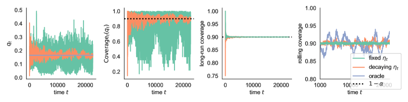
The experiments are run with two different choices of step size for online conformal: first, a fixed step size (); and second, a decaying step size ( with ). We also compare to an oracle method, where online conformal is run with in place of at each time , and is chosen to be the value that gives average coverage over the entire sequence . All methods are run with .
4.1 Results
Figures 2 and 2 display the results of the experiment for the Elec2 data and the Imagenet data, respectively. We now discuss our findings.
The thresholds .
The first panel of each figure plots the value of the threshold over time . We can see that the procedure with a fixed step size has significantly larger fluctuations in the quantile value as compared to the decaying step size procedure.
The instantaneous coverage .
The second panel of each figure plots the value of the instantaneous coverage over time . For each dataset, since the true data distribution is unknown, we estimate using a holdout set. We observe that is substantially more stable for the decaying step size as compared to fixed step size in both experiments. While concentrates closely around the nominal level for decaying , for fixed the coverage level oscillates and does not converge.
Long-run coverage and rolling coverage.
The third panel of each figure plots the value of the long-run coverage, , over time . We see that the long-run coverage converges quickly to for all methods, and we cannot differentiate between them in this plot.
Consequently, in the fourth panel of each figure, we also plot the “rolling” coverage, which computes coverage rate averaged over a rolling window of 1000 time points. We can see that this measure is tighter around for the fixed step size procedure; for the decaying step size procedure, rolling coverage fluctuates more, but is not larger than the fluctuations for the oracle method. At first glance, it might appear that having lower variance in the rolling coverage indicates that the fixed step size procedure is actually performing better than decaying step size—but this is not the case. The low variance with fixed is due to overcorrecting. For example, if we have several miscoverage events in a row (which can happen by random chance, even with the oracle intervals), then the fixed-step-size method will necessarily return an overly wide interval (e.g., ) to give certain coverage at the next time step. Thus, the fixed-step-size method ensures low variance in rolling coverage at the cost of extremely high variance in the width and instantaneous coverage of the interval at each time . This type of overcorrection is undesirable.
4.2 Implementation details for Elec2 Time Series
The Elec2 (Harries et al., 1999) dataset is a time-series of 45312 hourly measurements of electricity demand in New South Wales, Australia. We use even-numbered time points as the time series, and odd-numbered time points as a holdout set for estimating . The demand measurements are normalized to lie in the interval . The covariate vector is the sequence of all previous demand values. The forecast is one-day-delayed moving average of (i.e., at time , our predicted value is given by the average of observations taken between 24 and 48 hours earlier), and the score is .

4.3 Implementation details for Imagenet
The Imagenet (Deng et al., 2009) is a standard computer vision dataset of natural images. We take the 50000 validation images of Imagenet 2012 and treat them as a time series for the purpose of evaluating our methods. Because the validation split of Imagenet is shuffled, this comprises an exchangeable time series. We use 45000 points for the time series, and the remaining 5000 points as a holdout set for estimating . As the score function, we use (here is the softmax score of the pretrained ResNet-152 model).
4.4 Additional experiments
As discussed in Section 2.2, in applications where the distribution of the data may drift or may have changepoints, it might be beneficial to allow to increase at times to allow for updates in the learning process. To study this empirically, in the Appendix, we include additional experiments in a broader range of settings—we test over 3000 real datasets, and compare the fixed step size method, the decaying step size method, and a “decay+adapt” version of our method where the sequence adapts to trends in the data (decaying if the distribution of the data appears stationary, but increasing if distribution shift is detected).
5 Proofs
In this section, we prove Theorems 1, 2, 3, and 4, and Propositions 1 and 3. All other results are proved in the Appendix.
5.1 Proof of Theorems 1 and 2
First, we need a lemma to verify that the values are uniformly bounded over all . This result is essentially the same as that in Lemma 4.1 of Gibbs and Candes (2021), except extended to the setting of decaying, rather than constant, step size. The proof is given in the Appendix.
Lemma 1.
Let be an arbitrary sequence of data points, and let be arbitrary functions. Let be an arbitrary nonnegative sequence, and fix an initial threshold .
Then online conformal prediction satisfies
| (8) |
where , and for each .
We are now ready to prove the theorems. As discussed earlier, Theorem 1 is simply a special case, so we only prove the more general result Theorem 2.
By definition of , we have for all . We then calculate
where the last step holds since are bounded by Lemma 1.
5.2 Proof of Proposition 3
First we prove that almost surely. Equivalently, for any fixed , we need to prove that .
We begin by constructing a useful coupling between the online conformal process, and a sequence of I.I.D. uniform random variables. For each , define
drawn independently for each after conditioning on all the data, . Since by construction, we can verify that .
Next fix any integer . Let be the event that
Since the ’s are I.I.D. uniform random variables, we have for each , and the events are mutually independent. Therefore, by the second Borel–Cantelli lemma, . Now we claim that
| (9) |
Suppose that holds and that for all in the range . Then by construction of the ’s, we have for all . Therefore by (4),
where the last step holds by our choice of , together with the fact that by Lemma 1. But since the score function takes values in by assumption, we therefore have . Therefore, we have verified the claim (9).
Since occurs for infinitely many , almost surely, by (9) we therefore have , almost surely, as desired. Since is arbitrary, this completes the proof that almost surely.
Finally, a similar argument verifies almost surely.
5.3 Proof of Proposition 1
Since , we have , for each . By Proposition 3, and , almost surely. Since we have assumed that is a rational number, by the definition of the procedure (4), all values must lie on a discrete grid (i.e., if for some integers then, for all , must be an integer multiple of ). Moreover, by Lemma 1, is uniformly bounded above and below for all , so can only take finitely many values. This implies also can take only finitely many values, and in particular, this means that if (respectively, if ) then (respectively, ) for infinitely many .
5.4 Proofs of Theorems 3 and 4
We observe that Theorem 3 is simply a special case of Theorem 4 (obtained by taking for all ), so we only need to prove Theorem 4.
First, consider the sequence
Define events , the event that exists, and , the event that . In the Appendix, we will verify that
| (10) |
i.e., , using martingale theory.
To establish the theorem, then, it suffices for us to verify that on the event , it holds that . From this point on, we assume that and both hold.
Fix any . Since is monotone, it can have at most countably infinitely many discontinuities. Without loss of generality, then, we can assume that this map is continuous at and at (by taking a smaller value of if needed).
First, since converges, we can find some finite time such that
| (11) |
Moreover, since , we have and so we can find some finite time such that for all . Furthermore, on , we have , at each . Thus we can find some finite time and some such that
| (12) |
for all (we are using the fact that by (6)). Similarly we can find a finite and some such that for all . Let .
We will now split into cases. If it does not hold that for all sufficiently large , then one of the following cases must hold:
-
•
Case 1a: for all .
-
•
Case 1b: for all .
-
•
Case 2a: for some , it holds that and .
-
•
Case 2b: for some , it holds that and .
We now verify that each case is impossible.
Case 1a is impossible.
We have
where the last step holds since for , and is nondecreasing, and so we have
| (13) |
by (12). Since , we therefore have that , which is a contradiction.
Case 1b is impossible.
This proof is analogous to the proof for Case 1a.
Case 2a is impossible.
First, by assumption for this case, we can find a unique time such that
In other words, is the last time before time when the threshold is . Then we have
But since (because ), we have therefore reached a contradiction.
Case 2b is impossible.
This proof is analogous to the proof for Case 2a.
We have verified that all four cases are impossible. Therefore, for all sufficiently large . Since is arbitrarily small, this completes the proof.
6 Discussion
Our paper analyzes online conformal prediction that with a decaying step size, enabling simultaneous guarantees of convergence for I.I.D. sequences and long-run coverage for adversarial ones. Moreover, it helps further unify online conformal prediction with online learning and online convex optimization, since decaying step sizes are known to have desirable properties and hence standard for the latter. Of course, the usefulness of the method will rely on choosing score functions that are well suited to the (possibly time-varying) data distribution, and choosing step sizes that decay at an appropriate rate and perhaps adapt to the level of distribution shift—building a better understanding of how to make these choices in practice is crucial for achieving informative and stable prediction intervals. Many additional open questions about extending the methodology to broader settings and understanding connections to other tools remain. In particular, we expect fruitful avenues of future inquiry would be: (1) to extend this analysis to online risk control, as in Feldman et al. (2021); (2) to adapt our analysis of Theorem 3 to deal with stationary or slowly moving time-series which may not be I.I.D. but are slowly varying enough to permit estimation; and (3) to further understand the connection between this family of techniques and the theory of online learning.
Acknowledgements
The authors thank Isaac Gibbs, Ryan Tibshirani, and Margaux Zaffran for helpful feedback on this work. R.F.B. was partially supported by the National Science Foundation via grant DMS-2023109, and by the Office of Naval Research via grant N00014-20-1-2337.
References
- Angelopoulos and Bates [2023] Anastasios N Angelopoulos and Stephen Bates. Conformal prediction: A gentle introduction. Foundations and Trends® in Machine Learning, 16(4):494–591, 2023.
- Angelopoulos et al. [2023] Anastasios N. Angelopoulos, Emmanuel Candes, and Ryan Tibshirani. Conformal PID control for time series prediction. In Neural Information Processing Systems, 2023.
- Barber et al. [2022] Rina Foygel Barber, Emmanuel J Candes, Aaditya Ramdas, and Ryan J Tibshirani. Conformal prediction beyond exchangeability. arXiv:2202.13415, 2022.
- Bastani et al. [2022] Osbert Bastani, Varun Gupta, Christopher Jung, Georgy Noarov, Ramya Ramalingam, and Aaron Roth. Practical adversarial multivalid conformal prediction. Advances in Neural Information Processing Systems, 35:29362–29373, 2022.
- Bhatnagar et al. [2023] Aadyot Bhatnagar, Huan Wang, Caiming Xiong, and Yu Bai. Improved online conformal prediction via strongly adaptive online learning. arXiv preprint arXiv:2302.07869, 2023.
- Biau and Patra [2011] Gérard Biau and Benoît Patra. Sequential quantile prediction of time series. IEEE Transactions on Information Theory, 57(3):1664–1674, 2011.
- Bubeck and Slivkins [2012] Sébastien Bubeck and Aleksandrs Slivkins. The best of both worlds: Stochastic and adversarial bandits. In Conference on Learning Theory, pages 42–1. JMLR Workshop and Conference Proceedings, 2012.
- Cesa-Bianchi and Lugosi [2006] Nicolo Cesa-Bianchi and Gábor Lugosi. Prediction, learning, and games. Cambridge university press, 2006.
- Chen et al. [2023] Sijia Chen, Wei-Wei Tu, Peng Zhao, and Lijun Zhang. Optimistic online mirror descent for bridging stochastic and adversarial online convex optimization. In International Conference on Machine Learning, pages 5002–5035. PMLR, 2023.
- Chernozhukov et al. [2018] Victor Chernozhukov, Kaspar Wüthrich, and Zhu Yinchu. Exact and robust conformal inference methods for predictive machine learning with dependent data. In Conference On Learning Theory, pages 732–749. PMLR, 2018.
- Cramer et al. [2022] Estee Y Cramer, Evan L Ray, Velma K Lopez, Johannes Bracher, Andrea Brennen, Alvaro J Castro Rivadeneira, Aaron Gerding, Tilmann Gneiting, Katie H House, Yuxin Huang, et al. Evaluation of individual and ensemble probabilistic forecasts of covid-19 mortality in the united states. Proceedings of the National Academy of Sciences, 119(15):e2113561119, 2022.
- Daniely et al. [2015] Amit Daniely, Alon Gonen, and Shai Shalev-Shwartz. Strongly adaptive online learning. In International Conference on Machine Learning, pages 1405–1411. PMLR, 2015.
- Dann et al. [2023] Christoph Dann, Chen-Yu Wei, and Julian Zimmert. Best of both worlds policy optimization. In International Conference on Machine Learning, pages 6968–7008. PMLR, 2023.
- Deng et al. [2009] Jia Deng, Wei Dong, Richard Socher, Li-Jia Li, Kai Li, and Li Fei-Fei. Imagenet: A large-scale hierarchical image database. In 2009 IEEE conference on computer vision and pattern recognition, pages 248–255, 2009.
- Feldman et al. [2021] Shai Feldman, Stephen Bates, and Yaniv Romano. Improving conditional coverage via orthogonal quantile regression. In Advances in Neural Information Processing Systems, 2021.
- Feldman et al. [2023] Shai Feldman, Liran Ringel, Stephen Bates, and Yaniv Romano. Achieving risk control in online learning settings. Transactions on Machine Learning Research, 2023.
- Foreman-Mackey et al. [2017] Daniel Foreman-Mackey, Eric Agol, Sivaram Ambikasaran, and Ruth Angus. Fast and scalable Gaussian process modeling with applications to astronomical time series. The Astronomical Journal, 154(6):220, 2017.
- Foster and Vohra [1998] Dean P Foster and Rakesh V Vohra. Asymptotic calibration. Biometrika, 85(2):379–390, 1998.
- Gibbs and Candes [2021] Isaac Gibbs and Emmanuel Candes. Adaptive conformal inference under distribution shift. In M. Ranzato, A. Beygelzimer, Y. Dauphin, P.S. Liang, and J. Wortman Vaughan, editors, Advances in Neural Information Processing Systems, volume 34, pages 1660–1672. Curran Associates, Inc., 2021.
- Gibbs and Candès [2022] Isaac Gibbs and Emmanuel Candès. Conformal inference for online prediction with arbitrary distribution shifts. arXiv preprint arXiv:2208.08401, 2022.
- Gradu et al. [2023] Paula Gradu, Elad Hazan, and Edgar Minasyan. Adaptive regret for control of time-varying dynamics. In Learning for Dynamics and Control Conference, pages 560–572. PMLR, 2023.
- Harries et al. [1999] Michael Harries, New South Wales, et al. Splice-2 comparative evaluation: Electricity pricing. 1999.
- Jin et al. [2021] Tiancheng Jin, Longbo Huang, and Haipeng Luo. The best of both worlds: stochastic and adversarial episodic MDPs with unknown transition. Advances in Neural Information Processing Systems, 34:20491–20502, 2021.
- Koenker and Bassett Jr [1978] Roger Koenker and Gilbert Bassett Jr. Regression quantiles. Econometrica: Journal of the Econometric Society, 46(1):33–50, 1978.
- Koolen et al. [2016] Wouter M Koolen, Peter Grünwald, and Tim Van Erven. Combining adversarial guarantees and stochastic fast rates in online learning. Advances in Neural Information Processing Systems, 29, 2016.
- Lin et al. [2022] Zhen Lin, Shubhendu Trivedi, and Jimeng Sun. Conformal prediction with temporal quantile adjustments. Advances in Neural Information Processing Systems, 35:31017–31030, 2022.
- Lindemann et al. [2023] Lars Lindemann, Matthew Cleaveland, Gihyun Shim, and George J Pappas. Safe planning in dynamic environments using conformal prediction. IEEE Robotics and Automation Letters, 2023.
- Mykland [2003] Per Aslak Mykland. Financial options and statistical prediction intervals. The Annals of Statistics, 31(5):1413–1438, 2003.
- Noarov et al. [2023] Georgy Noarov, Ramya Ramalingam, Aaron Roth, and Stephan Xie. High-dimensional unbiased prediction for sequential decision making. In OPT 2023: Optimization for Machine Learning, 2023.
- Robinson [1978] JA Robinson. Sequential choice of an optimal dose: A prediction intervals approach. Biometrika, 65(1):75–78, 1978.
- Tian et al. [2022] Qinglong Tian, Daniel J Nordman, and William Q Meeker. Methods to compute prediction intervals: A review and new results. Statistical Science, 37(4):580–597, 2022.
- Vovk [2002] Vladimir Vovk. On-line confidence machines are well-calibrated. In The 43rd Annual IEEE Symposium on Foundations of Computer Science, pages 187–196. IEEE, 2002.
- Vovk et al. [2005] Vladimir Vovk, Alex Gammerman, and Glenn Shafer. Algorithmic Learning in a Random World. Springer, 2005. doi: 10.1007/b106715.
- Xu and Xie [2021] Chen Xu and Yao Xie. Conformal prediction interval for dynamic time-series. In International Conference on Machine Learning, pages 11559–11569. PMLR, 2021.
- Xu and Xie [2023] Chen Xu and Yao Xie. Sequential predictive conformal inference for time series. In International Conference on Machine Learning, pages 38707–38727. PMLR, 2023.
- Zaffran et al. [2022] Margaux Zaffran, Olivier Féron, Yannig Goude, Julie Josse, and Aymeric Dieuleveut. Adaptive conformal predictions for time series. In International Conference on Machine Learning, pages 25834–25866. PMLR, 2022.
- Zimmert and Seldin [2021] Julian Zimmert and Yevgeny Seldin. Tsallis-inf: An optimal algorithm for stochastic and adversarial bandits. Journal of Machine Learning Research, 22(28):1–49, 2021.
- Zinkevich [2003] Martin Zinkevich. Online convex programming and generalized infinitesimal gradient ascent. In Proceedings of the 20th international conference on machine learning (icml-03), pages 928–936, 2003.
Appendix A Additional proofs
A.1 Proof of Lemma 1
The proof of this result is similar to the proof of Lemma 4.1 of Gibbs and Candes [2021]. We prove this by induction. First, by assumption, so (8) is satisfied at time . Next fix any and assume lies in the range specified in (8), and consider . We now split into cases:
-
•
If , then we have
-
•
If , then we must have . Then , and so
-
•
If , then we must have . Then , and so
In all cases, then, (8) holds for in place of , which completes the proof.
A.2 Proof of 10
We need to prove that converges almost surely (note that the limit of may be a random variable). For each , we have
since and are functions of and are therefore independent of . This proves that is a martingale with respect to the filtration generated by the sequence of data points. We also have , since we have assumed . This means that is a uniformly integrable martingale, and therefore, converges almost surely (to some random variable), by Doob’s second martingale convergence theorem.
A.3 Proofs of Corollaries 1 and 2
Using the notation defined in the proof of Theorem 4, suppose that events and both hold. Now we need to show that holds as well. Fix any . Since has a continuous distribution, the map is continuous, and so we can find some such that
Moreover, , since the distribution of is continuous and is its -quantile, so we have
Next, by Theorem 4, for all sufficiently large , we have
By definition of the event , for all sufficiently large we have
and
Then, combining all of these calculations, for all sufficiently large we have
where the first step holds since , and is nondecreasing. Similarly, for all sufficiently large it holds that
Since is arbitrary, this completes the proof.
A.4 Proof of Proposition 2
By Lemma 1, for all (since for all ). Since , we therefore have almost surely for all . We also have and , since the density of is supported on and must integrate to .
Next, by the assumptions of the proposition, for any , if then
while if then
Either way, then, if then
A similar calculations shows that if , then
Defining , we therefore have
| (14) |
whenever . Note that we must have , by construction.
Next, from the update step (4), we have
Since , we then calculate
and
Therefore,
where the last step holds by (14) above. After marginalizing, then,
Next recall for each . Fix some that satisfies . First, since for all as above, by choosing we must have for all , almost surely. Next, for each , we proceed by induction. Assume . Then
where the last step holds as long as we choose . And, since , we have
where the last step holds since is convex, with derivative . Therefore, we have verified that , as desired.
Appendix B Additional experiments

We compare against two additional methods: first, “decay+adapt”, a variant of our procedure that decays until it detects a change point, then resets the learning rate. Change points are identified when at least consecutive miscoverage events or events are observed in a row (we set these constants to 10 and 30 by default, respectively). When a change point is identified, the learning rate is reset to , where is the time at which the changepoint is detected and . In these experiments, like in the main text, we set .
We additionally compare against DTACI Gibbs and Candès [2022], an adaptive-learning-rate variant of ACI that uses multiplicative weights to perform the updates (see Gibbs and Candès [2022] for further details.)
We compare these methods on a dataset of over 3000 time series subsampled from the M4 time series dataset. This dataset is a diverse array of time series with varying numbers of samples and distribution shifts. Code is available in our GitHub repository to run on all 100,000 time series in M4; here, we show results on the first 3000.
Finally, to showcase the conceptual differences between the standard decaying learning rate sequence and the ‘decay+adapt’ method, we display a simulated score sequence in Figure 4. Here, the scores are simulated from , where for the first thousand time steps, for the second thousand, for the third thousand, and for the final thousand. Especially towards the end of the time series, ‘decay+adapt’ can more quickly adjust to the change points.
| method | coverage | variance | MSE | infinite sets |
|---|---|---|---|---|
| DTACI | 0.895491 | 4.107740 | 5.439935 | 0.036584 |
| decay+adapt | 0.885174 | 1.144337 | 1.967552 | 0.005011 |
| decaying | 0.900495 | 1.320579 | 2.366297 | 0.006883 |
| fixed | 0.901636 | 1.580243 | 2.922989 | 0.011179 |
