One vanishing minor in neutrino mass matrix using trimaximal mixing
Abstract
We investigate the implications of one vanishing minor in neutrino mass matrix using trimaximal mixing matrix. In this context, we analyse all six patterns of one vanishing minor zero in neutrino mass matrix and present correlations of the neutrino oscillation parameters. All the six patterns are found to be phenomenologically viable with the present neutrino oscillation data. We also predict the values of effective Majorana mass, the effective electron anti-neutrino mass and the total neutrino mass for all the patterns. The value obtained for the effective neutrino mass is within the reach future neutrinoless double decay experiments. We also propose a flavor model where such patterns can be generated within the seesaw model.
pacs:
14.60.Pq, 14.60.St, 23.40.−sI Introduction
Evidence of neutrino oscillations observed in multitude of experiments confirms that neutrinos mix with each other and have non zero mass Super-Kamiokande:1998kpq . Neutrino oscillation phenomena can be parametrized in terms of six independent parameters, namely three mixing angles , one Dirac CP violating phase , and two mass squared differences . Although we have very precise values of the mixing angles and the absolute value of the mass squared differences, there are still some unknowns such as the octant of , and the sign of . There are two possible mass ordering of the neutrino mass spectrum: normal mass ordering (NO) and inverted mass ordering (IO) depending on the sign of .
Neutrino oscillation experiments are sensitive only to the mass squared differences. They can not provide any information regarding the absolute mass scale of neutrinos which is one of the most sought after questions in particle physics today. Knowledge of the absolute mass scale of neutrinos is of great importance not only in particle physics but also in understanding the large scale structure of our universe. Neutrinos possess very tiny mass and unlike all other fermions in the Standard Model (SM), they do not seem to get their mass through Higgs mechanism. Hence, it may, in principle, help shape our understanding of the origin of particle mass which is still one of the most fundamental questions of particle physics. Unlike all other fermions in the SM, we observe only left handed neutrinos and right handed anti-neutrinos. We have not found any right handed neutrino and left handed anti-neutrino so far in experiments. This brings us to the next relevant question whether neutrino is a Dirac particle or a Majorana particle. Neutrino interactions could violate CP as well which will be crucial in explaining the matter antimatter asymmetry in the universe. Moreover, there could be additional sterile neutrinos.
There are several experimental efforts to find the absolute mass of the neutrino. The decay experiment performed at KATRIN can, in principle, measure the effective electron anti-neutrino mass by studying the end point region of the decay spectrum. This is completely model independent determination, i.e, it depends neither on any cosmological models nor on the nature of neutrinos. At present, the improved upper bound on the effective electron anti-neutrino mass is reported to be at confidence level. The KATRIN experiment will continue to take data over the next several years and it is expected that the mass sensitivity will reach up to . Future experiments like Project Project8:2022wqh , designed to measure the absolute mass scale of the neutrino, hopes to reach a goal of neutrino mass sensitivity. Indirectly, one can have information on neutrino mass from cosmological observations. These cosmological observations are sensitive to the total neutrino mass and to the number of neutrino species. There are several results related to the total neutrino mass coming from various cosmological observations. Most of these indirect methods put a limit on the total neutrino mass to be less than . These results are, however, model dependent. They rely heavily on several cosmological assumptions. Current upper bound on the total neutrino mass is reported by the Planck satellite to be at confidence level combining BAO data with CMB data Zhang:2020mox . If KATRIN’s mass sensitivity reach up to in future, it can put severe constraint on several cosmological models. Rare double decay process with two anti neutrinos in the final state is allowed in the SM. In general double beta decay processes are powerful probes of beyond the SM physics. More specifically, if one observes neutrinoless double decay in experiments, it would confirm that neutrinos are Majorana in nature. One can determine the effective Majorana mass by studying neutrinoless double beta decay. There exists several limits on the value of using different isotopes. At present, the best limits are reported to be , and GERDA:2013vls ; CUORE:2015hsf ; EXO-200:2014ofj ; KamLAND-Zen:2012mmx , respectively.
There are several theoretical efforts in explaining the origin of neutrino mass. The most natural way to understand neutrino mass is through seesaw mechanism. The neutrino mass matrix in the framework of Type-I seesaw mechanism is given by , where is the Dirac neutrino mass matrix and is the Majorana mass matrix of the right handed neutrinos. Phenomenology of Majorana neutrino mass matrix has been studied extensively assuming zero textures of the neutrino mass matrix which may be realised from the zeros in or . In literature, there have been phenomenological studies with texture one-zero Lashin:2011dn ; Singh:2018tqu ; Gautam:2018izb , two-zeros Frampton:2002yf ; Xing:2002ta ; Xing:2002ap ; Lavoura:2004tu ; Dev:2006qe ; Kumar:2011vf ; Fritzsch:2011qv ; Ludl:2011vv ; Meloni:2012sx ; Grimus:2012zm ; Dev:2014dla ; Gautam:2016qyw ; Channey:2018cfj ; Singh:2019baq and more within the context of Pontecorvo Maki Nakagawa Sakata (PMNS), tribimaximal (TB) and trimaximal (TM) mixing matrix. Similarly, in Ref. Lashin:2007dm ; Lashin:2009yd ; Dev:2010if ; Dev:2010pf ; Tavartkiladze:2022pzf ; Araki:2012ip , the authors have studied the phenomenological implication of vanishing minors in the neutrino mass matrix. Moreover, in Ref. Liao:2013saa ; Dev:2013xca ; Wang:2013woa ; Whisnant:2015ovx ; Dev:2015lya ; Wang:2016tkm and Ref. Goswami:2008uv ; Dev:2009he ; Dev:2010pe ; Liu:2013oxa ; Dev:2013nua , the authors have explored the implication of cofactor zero and hybrid texture of the neutrino mass matrix. In case of zero textures, it is found that three or more zeros in neutrino mass matrix can not accommodate the current neutrino oscillation data. In Ref. Frampton:2002yf , the authors have found that out of fifteen possible two texture zeros cases only seven cases with PMNS mixing are allowed experimentally. Also out of fifteen possible two cofactors zero patterns only seven patterns are acceptable Lashin:2007dm . In case of TM mixing along with magic symmetry Gautam:2016qyw , the authors have found that only two cases are valid for two texture zero. TM mixing with one texture zero was studied in Ref. Gautam:2018izb and found that all six patterns are compatible with current neutrino oscillation data. For TB mixing along with the condition of texture zeros or vanishing minor Dev:2010pf only five patterns are allowed. In this work we study the implication of one vanishing minor in the neutrino mass matrix using trimaximal mixing.
Our paper is organized as follows. In Section. II, we briefly discuss the neutrino mass matrix using trimaximal mixing matrix. We find all the mixing parameters such as , , and the CP violating parameter in terms of the unknown parameters and of the trimaximal mixing matrix. In Section. III, we describe the formalism of one vanishing minor in neutrino mass matrix and identify all the possible patterns of one vanishing minor. We provide all the detail numerical analysis and discussion of each pattern in Sections. IV and V. The fine-tuning of neutrino mass matrix is presented in Section. VI. In Section. VII, we present the symmetry realization and conclude in Section. VIII.
II neutrino mass matrix
The most widely studied lepton flavor mixing is TB mixing pattern Harrison:2002er ; Harrison:2002kp ; Xing:2002sw ; Harrison:2003aw introduced by Harrison, Perkins and Scott. TB mixing pattern provides remarkable agreement with the atmospheric and solar neutrino oscillation data. The TB mixing pattern is given by
| (1) |
The TB mixing matrix possesses two types of symmetries: symmetry and magic symmetry. Although TB mixing matrix correctly predicted the value of atmospheric mixing angle and the solar mixing angle , it, however, failed to explain a non zero value of the reactor mixing angle that was experimentally confirmed by T2K T2K:2011ypd , MINOS MINOS:2011amj , Double Chooz DoubleChooz:2011ymz , Daya Bay DayaBay:2012fng and RENO RENO:2012mkc experiments. The possibility of an exact symmetry in the mass matrix was completely ruled out by a relatively large value of . Modifications in the TB mixing pattern Kumar:2010qz ; He:2011gb ; Grimus:2008tt was made to accommodate the present data. The TM mixing matrix was constructed by multiplying the TB mixing matrix by an unitary matrix and can be written as
| (2) |
and
| (3) |
where and are two free parameters. The neutrino mass matrix corresponding to TM mixing matrix can be written as
| (4) |
where is the diagonal matrix containing three mass state, and is the phase matrix written as
| (5) |
Here and are the two CP violating Majorana phases.
II.1 TM1 Mixing matrix
With TM1 mixing matrix, the elements of neutrino mass matrix can be written as
| (6) |
The three neutrino mixing angles , and can be expressed in terms of and , the free parameters of the TM1 matrix, as
| (7) | |||||
where and for . Using the standard parametrization of the PMNS matrix, the Jarlskog invariant, a measure of CP violation, is defined as Jarlskog:1985ht
| (8) |
Again, using the elements from TM1 mixing matrix, the Jarlskog invariant can be expressed as
| (9) |
Combining Eq. 8 and Eq. 9, we can write in terms of and as
| (10) |
The nature of neutrino can be determined from the effective Majorana mass term. It also measures the rate of neutrinoless double beta decay. The effective Majorana mass for the TM1 mixing matrix can be written as
| (11) |
Similarly, the effective electron anti-neutrino mass can be expressed as
| (12) |
II.2 TM2 Mixing matrix
Using TM2 mixing matrix, we can write the elements of neutrino mass matrix as
| (13) |
The three neutrino mixing angles , and can be expressed as
| (14) |
Again, using the elements from TM2 mixing matrix, the Jarlskog invariant can be expressed as
| (15) |
We can express the Dirac CP violating parameter in terms of and as
| (16) |
The effective Majorana mass for the TM2 mixing matrix can be written as
| (17) |
The effective electron anti-neutrino mass can be expressed as
| (18) |
III One vanishing minor in neutrino mass matrix
There are six independent minors corresponding to six independent elements in the neutrino mass matrix. We denote the minor corresponding to element of as . The six possible patterns of one minor zero in neutrino mass matrix are listed in Table. 1.
| Pattern | Constraining equation |
|---|---|
| I | |
| II | |
| III | |
| IV | |
| V | |
| VI |
The condition for one vanishing minor can be written as
| (19) |
More specifically, we can write Eq. 19 in terms of a complex equation as
| (20) |
where
| (21) |
with as the cyclic permutation of . Using Eq. 20, one can write the two mass ratios as
| (22) |
The value of , and can be calculated using Eq. III and mass square difference . That is
| (23) |
Similarly, the ratio of squared mass difference is defined as
| (24) |
where and represent solar and atmospheric mass squared difference, respectively. Value of is determined by using the measured values of and reported in Ref. Esteban:2020cvm .
IV Results and discussion
For our numerical analysis, we use the measured values of the oscillation parameters reported in Ref. Esteban:2020cvm . For completeness, we report them in Table. 2.
| parameter | Normal ordering(best fit) | inverted ordering ( |
|---|---|---|
| bfp ranges | bfp ranges | |
| 31.27 35.86 | 31.27 35.87 | |
| 39.5 52.0 | 39.8 52.1 | |
| 8.20 8.97 | 8.24 8.98 | |
| 105 405 | 192 361 | |
| 6.82 8.04 | 6.82 8.04 | |
| +2.431 +2.599 | -2.584 -2.413 |
We wish to find the value of the unknown parameters and . It is evident from Eq. 7 and Eq. II.2 that the neutrino oscillation parameters and depend only on . To find the best fit value of , we perform a naive analysis. The relevant is defined as
| (25) |
where . Here represents the theoretical value of and represents measured central value of . The corresponding uncertainties in the measured value of is represented by .
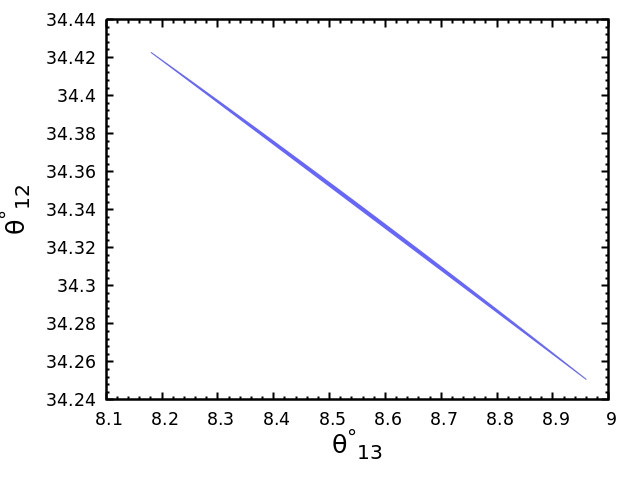
For the TM1 mixing matrix, the best fit value of is obtained to be . The corresponding best fit values of and are and , respectively. The allowed range of is found to be . Using the allowed range of , we obtain the allowed ranges of and to be and , respectively. We show in Fig. 1(a) the correlation of and for the TM1 mixing matrix. To see the variation of with , we use the allowed range of and vary within its full range from to . We show in Fig. 1(b) the variation of as a function of the unknown parameter . We also obtain the best fit value of by using the measured best fit value of . The best fit value is shown with a ’’ mark in Fig. 1(b). The best fit values of corresponding to the best fit value of are and , respectively. We show the variation of and as a function of in Fig. 1(c) and Fig. 1(d), respectively. It is observed that the Jarlskog rephasing invariant and the Dirac CP violating phase are restricted to two regions. The corresponding best fit values of and are and , respectively. We also obtain the allowed ranges of and to be and , respectively.


For TM2 mixing matrix, the best fit value of is obtained to be . The corresponding best fit values of and are and , respectively. The allowed range of is found to be . Using the allowed range of , we obtain the allowed ranges of and to be and , respectively. It should be noted that although the allowed range of obtained with TM2 mixing matrix is consistent with the experimental range, the best fit value obtained for , however, deviates from the experimental best fit value at more than significance. This is quite a generic feature of TM2 mixing matrix because, by default, value of will be greater than or equal to the value obtained in case of TB mixing matrix. We show in Fig. 2(a) the correlation of and for the TM2 mixing matrix.
To see the variation of with , we use the allowed range of and vary within its full range from to . We show in Fig. 2(b) the variation of as a function of the unknown parameter . The best fit value is shown with a ’’ mark in Fig. 2(b). We obtain the best fit value of by using the measured best fit value of . The best fit values of corresponding to the best fit value of are and , respectively. We get two best fit values of because is invariant under the transformation which is evident from Eq. 7 and Eq. II.2. We also show the variation of and as a function of in Fig. 2(c) and Fig. 2(d), respectively. It is observed that the Jarlskog rephasing invariant and the Dirac CP violating phase are restricted to two regions. The corresponding best fit values of and are and , respectively. We also obtain the allowed ranges of and to be and , respectively.


In case of inverted mass ordering the allowed range of are found to be and for both TM1 and TM2 mixing matrix, respectively. Using the allowed range of , we obtain the allowed ranges of to be and , respectively for both TM1 and TM2 mixing matrix. The allowed ranges of to be and , respectively for both TM1 and TM2 mixing matrix. It is to be noted that the mixing angles are almost similar for both the normal and inverted mass ordering. So for our later discussion we will use the values of mixing angles for the normal mass ordering reported in Ref. Esteban:2020cvm .
V Phenomenology of one vanishing minor
We wish to investigate the phenomenological implication of one vanishing minor in the neutrino mass matrix on the total neutrino mass, the effective Majorana mass term and the electron anti-neutrino mass. It is evident from Eq. III that neutrino mass depends on , , , and the mass squared difference . We use the best fit value and the allowed range of and of section. IV that are determined by the measured values of the mixing angles , and . The two unknown Majorana phases and are varied within their full range from to . Moreover, we use the allowed ranges of and to constrain the values of the neutrino masses. Now we proceed to analyse all the six patterns of one vanishing minor one by one.
V.1 Pattern I:
let us first consider minor zero for the element of the neutrino mass matrix. The equation corresponding to this pattern can be expressed in terms of the elements of the neutrino mass matrix as
| (26) |
Using Eq. III, the two mass ratios for TM1 can be expressed as
| (27) |
Similarly, for TM2 mixing matrix, the mass ratios can be expressed as
| (28) |
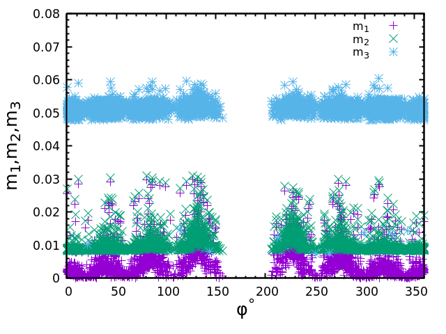
All the relevant expressions for and are reported in Eq. A and Eq. A of appendix A, respectively. We show the variation of neutrino masses , and as a function of in Fig 3(a) and Fig. 4(a) for TM1 and TM2 mixing matrix, respectively. It shows normal mass ordering for TM1 mixing matrix while for TM2 mixing matrix, it shows both normal and inverted mass ordering. The correlation of and for TM1 and TM2 mixing matrix are shown in Fig. 3(b) and Fig. 4(b), respectively. The vertical red line shows the upper bound of the total neutrino mass reported in Ref. Zhang:2020mox . The black, green and blue lines are the experimental upper bounds of the effective Majorana mass as reported in Ref. GERDA:2013vls ; CUORE:2015hsf ; EXO-200:2014ofj ; KamLAND-Zen:2012mmx . In Fig. 3(c) and Fig. 4(c), we have shown the correlation of with for TM1 and TM2 mixing matrix, respectively. It is observed that the total neutrino mass put severe constraint on effective Majorana mass and .


The range of the absolute neutrino mass scale, the effective Majorana neutrino mass and the effective electron anti-neutrino mass obtained for both the mixing matrix are listed in Table. 3. The calculated upper bound of is obtained to be of which is within the reach of neutrinoless double beta decay experiment. The calculated upper bound of may not be within the reach of KATRIN experiment. It may, however, be within the reach of next generation experiment such as Project 8. It should, however, be mentioned that once the total neutrino mass constraint is imposed, the calculated upper bound of and is found to be less than .
| Mixing | Mass | |||
|---|---|---|---|---|
| matrix | ordering | |||
| TM1 | NO | |||
| TM2 | NO | |||
| IO |
V.2 Pattern II:
The vanishing minor condition for this pattern corresponding to element (2,2) is given by
| (29) |
The two mass ratios for TM1 and TM2 mixing matrix can be expressed as
| (30) |
and
| (31) |
All the relevant expressions for and are reported in Eq. A and Eq. A of appendix A. We show the variation of neutrino masses , and as a function of in Fig 5(a) and Fig. 6(a) for TM1 and TM2 mixing matrix, respectively. It shows normal mass ordering for TM1 mixing matrix while for TM2 mixing matrix, it shows both normal and inverted mass ordering. The correlation of and for TM1 and TM2 mixing matrix are shown in Fig. 5(b) and Fig. 6(b), respectively. In Fig. 5(c) and Fig. 6(c), we have shown the correlation of with for TM1 and TM2 mixing matrix, respectively. The phenomenology of this pattern is quite similar to C33.


The allowed range of the absolute neutrino mass scale, the effective Majorana mass and the effective electron anti-neutrino mass for this pattern are listed in Table. 4.
| Mixing | Mass | |||
|---|---|---|---|---|
| matrix | ordering | |||
| TM1 | NO | |||
| TM2 | NO | |||
| IO |
V.3 Pattern III:
This pattern corresponds to the matrix element (3,1) of the neutrino mass matrix. The vanishing minor condition is given by
| (32) |
Using the elements from neutrino mass matrix, one can write the neutrino mass ratios for this pattern. With TM1 mixing matrix, we have
| (33) |
and for TM2 mixing matrix, we have
| (34) |
where all the relevant and are reported in Eq. A and Eq. A of appendix A. We show in Fig. 7(a) and Fig. 8(a) the correlation of neutrino masses , and with the unknown parameter for TM1 and TM2 mixing matrix. It shows both normal and inverted mass ordering for TM1 and TM2 mixing matrix. Similarly, the correlation of against for TM1 and TM2 mixing patterns are shown in Fig. 7(b) and Fig. 8(b),respectively. Moreover, in the Fig. 7(c) and Fig. 8(c), we have shown the correlation of with for TM1 and TM2, respectively.


The allowed ranges of the absolute neutrino mass, the effective Majorana mass and the effective electron anti-neutrino mass for both the maxing matrix are listed in the Table. 5.
| Mixing | Mass | |||
| matrix | ordering | |||
| TM1 | NO | |||
| IO | ||||
| TM2 | NO | |||
| IO |
V.4 Pattern IV:
The vanishing minor condition for this pattern corresponding to element (2,1) of the neutrino mass matrix is given by
| (35) |
The two neutrino mass ratios for this pattern for TM1 and TM2 mixing matrix are given by
| (36) |
and
| (37) |
where all the relevant and are reported in Eq. A and Eq. A of appendix A. In Fig. 9(a) and Fig. 10(a) we have shown the correlation of neutrino masses , and with the unknown parameter for TM1 and TM2 mixing matrix. It shows both normal and inverted mass ordering for TM1 and TM2 mixing matrix. The correlation of against for TM1 and TM2 mixing patterns are shown in Fig. 9(b) and Fig. 10(b),respectively. In the Fig. 9(c) and Fig. 10(c), we have shown the correlation of with for TM1 and TM2, respectively.


We also report the allowed ranges of the absolute neutrino mass, the effective Majorana mass and the effective electron anti-neutrino mass for both the maxing matrix in Table. 6. The phenomenology of this pattern is very similar to that of .
| Mixing | Mass | |||
| matrix | ordering | |||
| TM1 | NO | |||
| IO | ||||
| TM2 | NO | |||
| IO |
V.5 Pattern V:
The condition of vanishing minor for this pattern is given by
| (38) |
For this pattern, the two neutrino mass ratios for TM1 and TM2 mixing matrix are given by
| (39) |
and
| (40) |
respectively. The relevant expressions for and are are reported in Eq. A and Eq. A of appendix A. The correlation of neutrino masses , and with the unknown parameter are shown in Fig. 11(a) and Fig. 12(a), respectively for TM1 and TM2 mixing matrix. It is observed that, it shows normal mass ordering for TM1 mixing matrix, whereas, for TM2 mixing matrix, it shows both normal and inverted mass ordering. The correlation of and are shown in Fig. 11(b) and Fig. 12(b), respectively using TM1 and TM2 mixing matrix. In Fig. 11(c) and Fig. 12(c), we have shown the correlation of with using TM1 and TM2 mixing matrix, respectively.


The allowed ranges of all the relevant parameters such as the absolute neutrino mass, the effective Majorana mass and the effective electron anti-neutrino mass under normal and inverted ordering for both the mixing matrix are reported in Table. 7.
| Mixing | Mass | |||
|---|---|---|---|---|
| matrix | ordering | |||
| TM1 | NO | |||
| TM2 | NO | |||
| IO |
V.6 Pattern VI:
The vanishing minor condition for this pattern is given by
| (41) |
The two neutrino mass ratios can be obtained using the elements from neutrino mass matrix. For TM1 mixing matrix, we have
| (42) | |||||
and for TM2 mixing matrix, we have
| (43) |
Using Eq. 42, we obtain the mass relation for TM1 mixing matrix as
| (44) |
and using Eq. V.6, we obtain the mass relation for TM2 mixing matrix as
| (45) |
This pattern gives a clear inverted mass ordering for both TM1 and TM2 mixing matrix. The correlation of the neutrino masses , and for both the mixing patterns with the unknown parameter is shown in Fig. 13(a) and Fig. 14(a), respectively. The correlation of with for TM1 and TM2 are shown in Fig. 13(b) and Fig. 14(b), respectively. In Fig. 13(c) and Fig. 14(c), we have shown the correlation of with for TM1 and TM2 mixing matrix, respectively.
The allowed ranges of the absolute neutrino mass, the effective Majorana mass and the effective electron anti-neutrino mass obtained for both the mixing matrix are listed in the tables 8.
| Mixing | Mass | |||
|---|---|---|---|---|
| matrix | ordering | |||
| TM1 | IO | |||
| TM2 | IO |


VI Degree of Fine tuning in the neutrino mass matrix
In this section, we wish to determine whether the entries of the neutrino mass matrix are fine tuned or not. In order to determine the degree of fine tuning of the mass matrix elements, we define a parameter Altarelli:2010at ; Meloni:2012sx which is obtained as the sum of the absolute values of the ratios between each parameter and its error. We follow Ref. Altarelli:2010at ; Meloni:2012sx and define the fine tuning parameter as
| (46) |
where is the best fit values of the parameters. The error for each parameter is obtained from the shift of best fit value that changes the value by one unit keeping all other parameters fixed at their best fit values. To determine the best fit values of all the parameters, we perform a analysis of all the classes of one minor zero and find the . We define the as follows:
| (47) |
where and . Here and represent the theoretical value of and , respectively, whereas and represent measured central value of and , respectively. It should be noted that and depend on four unknown model parameters, namely , , and . Similarly, the uncertainties in the measured value of and are represented by and , respectively. The central values and the corresponding uncertainties in each parameter are reported in Table. 2.
We first compute which is defined as the sum of the absolute values of the ratios between the measured values of each parameter and its error from Table. 2. We obtain the value of to be around for both normal and inverted ordering case. The degree of fine tuning can be roughly estimated from the value of because if the value is large then a minimal variation of the corresponding parameters give large difference on the value of . Hence a large value of corresponds to a strong fine tuning of the mass matrix elements and vice versa. The value and the corresponding best fit values of the unknown parameters of the neutrino mass matrix , , , and the value of parameter for each patterns are listed in the Table. 9 and Table. 10 for the TM1 and TM2 mixing matrix respectively. We also report the best fit values of several observables such as , , , and for each pattern. For the patterns and , the results are for NO case and for the pattern , the results are for IO case. As the pattern follows the IO, the value obtained for this pattern is large for both TM1 and TM2 mixing matrix. The best fit values of the mixing angles , , and the mass squared differences , obtained for each pattern are compatible with the experimentally measured values reported in Table. 2.
| Type | |||||||||||
| Type | |||||||||||
In case of TM1 mixing matrix, pattern shows very good agreement with the data with a very small value. Although, the pattern also have same as pattern , it, however, has a much larger value compared to pattern . It can be concluded that for the pattern , there is a strong fine tuning among the elements of the mass matrix. Similarly, , and have larger value compared to pattern, although they have less value than . For , and also the degree of fine tuning among the mass matrix elements is very strong. Moreover, it is very clear from Table. 9 that all these patterns prefer the atmospheric mixing angle to be greater than . Based on the values, it is clear that it requires less fine tuning of the mass matrix elements for patterns and .
For the TM2 mixing matrix, the fine-tuned parameter is small for the patterns , , and . Among all these patterns has the lowest value. However, for patterns and , value is quite large and hence the degree of fine tuning among the elements of the mass matrix is quite strong for these patterns. All the patterns prefer the best fit value of to be larger than .
VII symmetry realization
The symmetry of one vanishing minor can be realized through type-I seesaw mechanism Minkowski:1977sc ; Mohapatra:1979ia along with Abelian symmetry. One vanishing minor in neutrino mass matrix can easily be obtained if one element in the Majorana matrix is zero along with diagonal Dirac mass matrix . In order to fulfil this condition, we need three right handed charged lepton , three right handed neutrinos and three left handed lepton doublets . We present the symmetry realization of pattern V. The symmetry of this pattern can be realized through the Abelian symmetry group that is discussed in Refs. Grimus:2004hf ; Dev:2010if .
The leptonic fields under transform as
| (48) |
where = . The bilinears and , where , relevant for and transform as , where
| (49) |
and the bilinears relevant for transform as , where
| (50) |
For each non zero element in , we need a scalar singlet and for each non zero element in or , we need Higgs scalar or , respectively. The scalar singlets get the vacuum expectation values (vevs) at the seesaw scale, while Higgs doublets get vevs at the electroweak scale. Under transformation, the sign of and changes, while other multiplets remain invariant. The diagonal charged lepton mass matrix can be obtained by introducing only three Higgs doublets namely , and , similarly, the diagonal Dirac neutrino mass matrix can be obtained by introducing three Higgs doublets , and . The non zero elements of can be obtained by introducing scalar fields , , , and which under transformation gets multiplied by , , , and , respectively. The Majorana mass matrix can be written as
| (51) |
This provides minor zero corresponding to (3,2) element in the neutrino mass matrix. Other patterns can also be realised similarly for different .
VIII conclusion
We explore the implication of one minor zero in the neutrino mass matrix obtained using trimaximal mixing matrix. There are total six possible patterns and all the patterns are found to be phenomenologically compatible with the present neutrino oscillation data. The two unknown parameters and of the trimaximal mixing matrix are determined by using the experimental values of the mixing angles , and . It is found that TM1 mixing matrix provides a better fit to the experimental results than TM2 mixing matrix. The Jarlskog invariant measure of CP violation is non zero for all the pattern, so they are necessarily CP violating. Patterns I, II and V show normal mass ordering for TM1 mixing matrix while these patterns show both normal and inverted mass ordering for TM2 mixing matrix. Patterns III and IV show both normal and inverted mass ordering for both TM1 and TM2 mixing matrix. Pattern VI predicts inverted mass ordering for both the mixing matrix. We predict the unknown parameters such as the absolute neutrino mass scale, the effective Majorana mass and the effective electron anti-neutrino mass using both TM1 and TM2 mixing matrix. The effective Majorana mass obtained for each pattern is within the reach of neutrinoless double beta decay experiment. Similarly, the value obtained for the effective electron anti-neutrino mass may be within the reach of future Project 8 experiment. We also discuss the fine tuning of the elements of the mass matrix for all the patterns by introducing a new parameter . We observe that for the pattern , the fine tuning among the elements of the mass matrix is small compared to other patterns. Moreover, we also discuss the symmetry realization of pattern V using Abelian symmetry group in the framework of type-I seesaw model which can be easily generalized to all the other patterns as well.
Appendix A
The coefficients in the mass ratios for the TM1 mixing matrix can be expressed in terms of the two unknown parameters and as
| (52) |
| (53) |
| (54) |
| (55) |
| (56) |
Similarly, the coefficients in the mass ratios for the TM2 mixing can be written as
| (57) |
| (58) |
| (59) |
| (60) |
| (61) |
References
-
(1)
Y. Fukuda et al. [Super-Kamiokande],
Phys. Rev. Lett. 81, 1562-1567 (1998)
doi:10.1103/PhysRevLett.81.1562
[arXiv:hep-ex/9807003 [hep-ex]].
-
(2)
A. A. Esfahani et al. [Project 8],[arXiv:2203.07349 [nucl-ex]].
-
(3)
M. Zhang, J. F. Zhang and X. Zhang,
Commun. Theor. Phys. 72, no.12, 125402 (2020)
[arXiv:2005.04647 [astro-ph.CO]].
-
(4)
M. Agostini et al. [GERDA],
Phys. Rev. Lett. 111, no.12, 122503 (2013)
doi:10.1103/PhysRevLett.111.122503
[arXiv:1307.4720 [nucl-ex]].
-
(5)
K. Alfonso et al. [CUORE],
Phys. Rev. Lett. 115, no.10, 102502 (2015)
doi:10.1103/PhysRevLett.115.102502
[arXiv:1504.02454 [nucl-ex]].
-
(6)
J. B. Albert et al. [EXO-200],
Nature 510, 229-234 (2014)
doi:10.1038/nature13432
[arXiv:1402.6956 [nucl-ex]].
-
(7)
A. Gando et al. [KamLAND-Zen],
Phys. Rev. Lett. 110, no.6, 062502 (2013)
doi:10.1103/PhysRevLett.110.062502
[arXiv:1211.3863 [hep-ex]].
-
(8)
E. I. Lashin and N. Chamoun,
Phys. Rev. D 85, 113011 (2012)
doi:10.1103/PhysRevD.85.113011
[arXiv:1108.4010 [hep-ph]].
-
(9)
M. Singh,
Adv. High Energy Phys. 2018, 2863184 (2018)
doi:10.1155/2018/2863184
[arXiv:1803.10735 [hep-ph]].
-
(10)
R. R. Gautam,
Phys. Rev. D 97, no.5, 055022 (2018)
doi:10.1103/PhysRevD.97.055022
[arXiv:1802.00425 [hep-ph]].
-
(11)
P. H. Frampton, S. L. Glashow and D. Marfatia,
Phys. Lett. B 536, 79-82 (2002)
doi:10.1016/S0370-2693(02)01817-8
[arXiv:hep-ph/0201008 [hep-ph]].
-
(12)
Z. z. Xing,
Phys. Lett. B 530, 159-166 (2002)
doi:10.1016/S0370-2693(02)01354-0
[arXiv:hep-ph/0201151 [hep-ph]].
-
(13)
Z. z. Xing,
Phys. Lett. B 539, 85-90 (2002)
doi:10.1016/S0370-2693(02)02062-2
[arXiv:hep-ph/0205032 [hep-ph]].
-
(14)
L. Lavoura,
Phys. Lett. B 609, 317-322 (2005)
doi:10.1016/j.physletb.2005.01.047
[arXiv:hep-ph/0411232 [hep-ph]].
-
(15)
S. Dev, S. Kumar, S. Verma and S. Gupta,
Phys. Rev. D 76, 013002 (2007)
doi:10.1103/PhysRevD.76.013002
[arXiv:hep-ph/0612102 [hep-ph]].
-
(16)
S. Kumar,
Phys. Rev. D 84, 077301 (2011)
doi:10.1103/PhysRevD.84.077301
[arXiv:1108.2137 [hep-ph]].
-
(17)
H. Fritzsch, Z. z. Xing and S. Zhou,
JHEP 09, 083 (2011)
doi:10.1007/JHEP09(2011)083
[arXiv:1108.4534 [hep-ph]].
-
(18)
P. O. Ludl, S. Morisi and E. Peinado,
Nucl. Phys. B 857, 411-423 (2012)
doi:10.1016/j.nuclphysb.2011.12.017
[arXiv:1109.3393 [hep-ph]].
-
(19)
D. Meloni and G. Blankenburg,
Nucl. Phys. B 867, 749-762 (2013)
doi:10.1016/j.nuclphysb.2012.10.011
[arXiv:1204.2706 [hep-ph]].
-
(20)
W. Grimus and P. O. Ludl,
J. Phys. G 40, 055003 (2013)
doi:10.1088/0954-3899/40/5/055003
[arXiv:1208.4515 [hep-ph]].
Dev:2015lya -
(21)
S. Dev, R. R. Gautam, L. Singh and M. Gupta,
Phys. Rev. D 90, no.1, 013021 (2014)
doi:10.1103/PhysRevD.90.013021
[arXiv:1405.0566 [hep-ph]].
-
(22)
R. R. Gautam and S. Kumar,
Phys. Rev. D 94, no.3, 036004 (2016)
[erratum: Phys. Rev. D 100, no.3, 039902 (2019)]
doi:10.1103/PhysRevD.94.036004
[arXiv:1607.08328 [hep-ph]].
-
(23)
K. S. Channey and S. Kumar,
J. Phys. G 46, no.1, 015001 (2019)
doi:10.1088/1361-6471/aaf55e
[arXiv:1812.10268 [hep-ph]].
-
(24)
M. Singh,
EPL 129, no.1, 1 (2020)
doi:10.1209/0295-5075/129/11002
[arXiv:1909.01552 [hep-ph]].
-
(25)
E. I. Lashin and N. Chamoun,
Phys. Rev. D 78, 073002 (2008)
doi:10.1103/PhysRevD.78.073002
[arXiv:0708.2423 [hep-ph]].
-
(26)
E. I. Lashin and N. Chamoun,
Phys. Rev. D 80, 093004 (2009)
doi:10.1103/PhysRevD.80.093004
[arXiv:0909.2669 [hep-ph]].
-
(27)
S. Dev, S. Verma, S. Gupta and R. R. Gautam,0
Phys. Rev. D 81, 053010 (2010)
doi:10.1103/PhysRevD.81.053010
[arXiv:1003.1006 [hep-ph]].
-
(28)
S. Dev, S. Gupta and R. R. Gautam,
Mod. Phys. Lett. A 26, 501-514 (2011)
doi:10.1142/S0217732311034906
[arXiv:1011.5587 [hep-ph]].
-
(29)
Z. Tavartkiladze,
Phys. Rev. D 106, no.11, 115002 (2022)
doi:10.1103/PhysRevD.106.115002
[arXiv:2209.14404 [hep-ph]].
-
(30)
T. Araki, J. Heeck and J. Kubo,
JHEP 07, 083 (2012)
doi:10.1007/JHEP07(2012)083
[arXiv:1203.4951 [hep-ph]].
-
(31)
J. Liao, D. Marfatia and K. Whisnant,
JHEP 09, 013 (2014)
doi:10.1007/JHEP09(2014)013
[arXiv:1311.2639 [hep-ph]].
-
(32)
S. Dev, R. R. Gautam and L. Singh,
Phys. Rev. D 87, 073011 (2013)
doi:10.1103/PhysRevD.87.073011
[arXiv:1303.3092 [hep-ph]].
-
(33)
W. Wang,
Eur. Phys. J. C 73, 2551 (2013)
doi:10.1140/epjc/s10052-013-2551-2
[arXiv:1306.3556 [hep-ph]].
-
(34)
K. Whisnant, J. Liao and D. Marfatia,
AIP Conf. Proc. 1604, no.1, 273-278 (2015)
doi:10.1063/1.4883441
-
(35)
S. Dev, L. Singh and D. Raj,
Eur. Phys. J. C 75, no.8, 394 (2015)
doi:10.1140/epjc/s10052-015-3569-4
[arXiv:1506.04951 [hep-ph]].
-
(36)
W. Wang, S. Y. Guo and Z. G. Wang,
Mod. Phys. Lett. A 31, no.13, 1650080 (2016)
doi:10.1142/S0217732316500802
-
(37)
S. Goswami, S. Khan and A. Watanabe,
Phys. Lett. B 693, 249-254 (2010)
doi:10.1016/j.physletb.2010.08.033
[arXiv:0811.4744 [hep-ph]].
-
(38)
S. Dev, S. Verma and S. Gupta,
Phys. Lett. B 687, 53-60 (2010)
doi:10.1016/j.physletb.2010.02.055
[arXiv:0909.3182 [hep-ph]].
-
(39)
S. Dev, S. Gupta and R. R. Gautam,
Phys. Rev. D 82, 073015 (2010)
doi:10.1103/PhysRevD.82.073015
[arXiv:1009.5501 [hep-ph]].
-
(40)
J. Y. Liu and S. Zhou,
Phys. Rev. D 87, no.9, 093010 (2013)
doi:10.1103/PhysRevD.87.093010
[arXiv:1304.2334 [hep-ph]].
-
(41)
S. Dev, R. R. Gautam and L. Singh,
Phys. Rev. D 88, 033008 (2013)
doi:10.1103/PhysRevD.88.033008
[arXiv:1306.4281 [hep-ph]].
-
(42)
P. F. Harrison, D. H. Perkins and W. G. Scott,
Phys. Lett. B 530, 167 (2002)
doi:10.1016/S0370-2693(02)01336-9
[arXiv:hep-ph/0202074 [hep-ph]].
-
(43)
P. F. Harrison and W. G. Scott,
Phys. Lett. B 535, 163-169 (2002)
doi:10.1016/S0370-2693(02)01753-7
[arXiv:hep-ph/0203209 [hep-ph]].
-
(44)
Z. z. Xing,
Phys. Lett. B 533, 85-93 (2002)
doi:10.1016/S0370-2693(02)01649-0
[arXiv:hep-ph/0204049 [hep-ph]].
-
(45)
P. F. Harrison and W. G. Scott,
Phys. Lett. B 557, 76 (2003)
doi:10.1016/S0370-2693(03)00183-7
[arXiv:hep-ph/0302025 [hep-ph]].
-
(46)
K. Abe et al. [T2K],
Phys. Rev. Lett. 107, 041801 (2011)
doi:10.1103/PhysRevLett.107.041801
[arXiv:1106.2822 [hep-ex]].
-
(47)
P. Adamson et al. [MINOS],
Phys. Rev. Lett. 107, 181802 (2011)
doi:10.1103/PhysRevLett.107.181802
[arXiv:1108.0015 [hep-ex]].
-
(48)
Y. Abe et al. [Double Chooz],
Phys. Rev. Lett. 108, 131801 (2012)
doi:10.1103/PhysRevLett.108.131801
[arXiv:1112.6353 [hep-ex]].
-
(49)
F. P. An et al. [Daya Bay],
Phys. Rev. Lett. 108, 171803 (2012)
doi:10.1103/PhysRevLett.108.171803
[arXiv:1203.1669 [hep-ex]].
-
(50)
J. K. Ahn et al. [RENO],
Phys. Rev. Lett. 108, 191802 (2012)
doi:10.1103/PhysRevLett.108.191802
[arXiv:1204.0626 [hep-ex]].
-
(51)
S. Kumar,
Phys. Rev. D 82, 013010 (2010)
[erratum: Phys. Rev. D 85, 079904 (2012)]
doi:10.1103/PhysRevD.82.013010
[arXiv:1007.0808 [hep-ph]].
-
(52)
X. G. He and A. Zee,
Phys. Rev. D 84, 053004 (2011)
doi:10.1103/PhysRevD.84.053004
[arXiv:1106.4359 [hep-ph]].
-
(53)
W. Grimus and L. Lavoura,
JHEP 09, 106 (2008)
doi:10.1088/1126-6708/2008/09/106
[arXiv:0809.0226 [hep-ph]].
-
(54)
C. Jarlskog,
Phys. Rev. Lett. 55, 1039 (1985)
doi:10.1103/PhysRevLett.55.1039
-
(55)
I. Esteban, M. C. Gonzalez-Garcia, M. Maltoni, T. Schwetz and A. Zhou,
JHEP 09, 178 (2020)
doi:10.1007/JHEP09(2020)178
[arXiv:2007.14792 [hep-ph]].NuFIT 5.0(2020), http://www.nu-fit.org.
- (56) G. Altarelli and G. Blankenburg, JHEP 03, 133 (2011) doi:10.1007/JHEP03(2011)133 [arXiv:1012.2697 [hep-ph]].
-
(57)
P. Minkowski,
Phys. Lett. B 67, 421-428 (1977)
doi:10.1016/0370-2693(77)90435-X.
-
(58)
R. N. Mohapatra and G. Senjanovic,
Phys. Rev. Lett. 44, 912 (1980)
doi:10.1103/PhysRevLett.44.912.
-
(59)
W. Grimus, A. S. Joshipura, L. Lavoura and M. Tanimoto,
Eur. Phys. J. C 36, 227-232 (2004)
doi:10.1140/epjc/s2004-01896-y
[arXiv:hep-ph/0405016 [hep-ph]].