One line to run them all: SuperEasy massive neutrino linear response in $N$-body simulations

To obtain a formal solution to this Poisson–Boltzmann system (2.1)–(2.2), we follow the prescription of [36] and Fourier-transform equation (2.1) according to $A(\vec{k})={\cal F}[A(\vec{x})]\equiv\int_{-\infty}^{\infty}A(\vec{x})\,e^{-i\vec{k}\cdot\vec{x}}\,\mathrm{d}^{3}x$. Rewriting the transformed equation in terms of a superconformal time variable defined as $s\equiv\int a^{-1}\mathrm{d}\tau$, we find

$$\frac{\partial{f}}{\partial s}+\frac{i\,\vec{k}\cdot\vec{p}}{m_{\nu}}{f}-im_{\nu}a^{2}(\vec{k}\,{\phi}\ast\nabla_{\!\vec{p}}\,{f})=0\,,$$

(2.5)

where $A(\vec{k})*B(\vec{k})\equiv\int{\rm d}^{3}k^{\prime}\,A(\vec{k}^{\prime})B(\vec{k}-\vec{k}^{\prime})$ denotes a convolution product. Observe that the convolution term is also the only instance of $\vec{k}$-mode coupling in equation (2.5). Therefore, we simplify it first by linearisation, i.e.,

	$\displaystyle\vec{k}\,{\phi}\ast\nabla_{\!\vec{p}}\,{f}\simeq$	$\displaystyle\,\vec{k}\,{\phi}\ast\nabla_{\!\vec{p}}\left(\bar{f}(p)\,\delta_{D}^{(3)}(\vec{k})\right)$		(2.6)
	$\displaystyle=$	$\displaystyle\,\vec{k}\,{\phi}\cdot\nabla_{\!\vec{p}}\,\bar{f}(p)\,,$

where $\delta^{(3)}_{D}(\vec{k})$ denotes a 3-dimensional Dirac delta distribution in $k$-space, Physically, the linearisation scheme (2.6) corresponds to assuming that gravitational clustering does not significantly distort the neutrino phase space density from its homogeneous expectation,

$$|\nabla_{\!\vec{p}}\,(f-\bar{f})|\ll|\nabla_{\!\vec{p}}\,\bar{f}|,$$

(2.7)

an assumption that should hold as long as the neutrino density contrast remains well below unity. We shall revisit this issue of linearisation in section 7.

Upon linearisation, the Fourier-space Boltzmann equation (2.5) now reduces to a first-order inhomogeneous differential equation of the form

$$\frac{\partial{f}}{\partial s}+\frac{i\vec{k}\cdot\vec{p}}{m_{\nu}}{f}-im_{\nu}a^{2}(\vec{k}\,{\phi}\cdot\nabla_{\!\vec{p}}\,\bar{f})=0\,.$$

(2.8)

Treating ${\phi}(\vec{k},s)$ as an external potential, equation (2.8) is formally solved by [36]

	$\displaystyle{f}(\vec{k},\vec{p},s)=$	$\displaystyle\,{f}(\vec{k},\vec{p},s_{\rm i})\,\text{exp}\!\left(-\frac{i\vec{k}\cdot\vec{p}}{m_{\nu}}(s-s_{\rm i})\right)$		(2.9)
		$\displaystyle\hskip 42.67912pt+im_{\nu}\vec{k}\cdot\nabla_{\!\vec{p}}\,\bar{f}\int_{s_{\rm i}}^{s}\mathrm{d}s^{\prime}\,a^{2}(s^{\prime})\,{\phi}(\vec{k},s^{\prime})\,\text{exp}\!\left(-\frac{i\vec{k}\cdot\vec{p}}{m_{\nu}}(s-s^{\prime})\right)\,.$

Physically, the solution to the homogeneous equation (i.e., the first term) corresponds to redistribution of the initial conditions at $s=s_{\rm i}$ in the neutrino sector via free-streaming. In contrast, the inhomogeneous solution (the second term) represents the neutrinos’ response to the formally external gravitational potential — hence the name “linear response”.

Then, integrating (2.9) in momentum as per equation (2.4), we find the neutrino density contrast ${\delta}_{\nu}(\vec{k},s)$ at the mode $\vec{k}$ and time $s$ to be [36]

$\displaystyle{\delta}_{\nu}(\vec{k},s)\simeq-k^{2}\int_{s_{\rm i}}^{s}\mathrm{d}s^{\prime}\,a^{2}(s^{\prime})\,\phi(\vec{k},s^{\prime})\,(s-s^{\prime})\,F\left[\frac{T_{\nu,0}k(s-s^{\prime})}{m_{\nu}}\right]\,,$

(2.10)

where

$\displaystyle F(q)\equiv\frac{m_{\nu}}{\bar{\rho}_{\nu}(s)}\int\mathrm{d}^{3}p\,\bar{f}(p)\,\text{exp}\left(-i\vec{q}\cdot\vec{p}/T_{\nu,0}\right)$

(2.11)

is effectively a Fourier transform of the homogeneous phase density $\bar{f}(p)$ in the comoving momentum variable $\vec{p}$ to a new variable $\vec{q}$. For a relativistic Fermi–Dirac distribution, $F(q)$ evaluates to

	$\displaystyle F(q)$	$\displaystyle=\frac{4}{3\zeta(3)}\sum_{n=1}^{\infty}(-1)^{n+1}\frac{n}{(n^{2}+q^{2})^{2}}$		(2.12)
		$\displaystyle=\frac{i}{12\zeta(3)q}\Bigg{[}\psi^{(1)}\left(\frac{1+iq}{2}\right)-\psi^{(1)}\left(\frac{1-iq}{2}\right)+\psi^{(1)}\left(-\frac{iq}{2}\right)-\psi^{(1)}\left(\frac{iq}{2}\right)\Bigg{]},$

with the Riemann zeta function $\zeta(3)\simeq 1.202$, and $\psi^{(i)}$ is a polygamma function of order $i$. Observe that in writing equation (2.10) we have also assumed the free-streaming redistribution term in equation (2.9) to integrate approximately to the homogeneous background density $\bar{\rho}_{\nu}(s)$, such that the final ${\delta}_{\nu}(\vec{k},s)$ depends only on its response to a formally external gravitational source.

Equation (2.10) is the starting point of all existing linear response calculations of nonrelativistic gravitational neutrino clustering in the literature. To distinguish it from the SuperEasy linear response method proposed in this work, we shall refer to it as “integral linear response” because of the remaining integral over time. Integral linear response (2.10) has been previously applied to the investigation of neutrino clustering around cosmic string loops [37], dark matter halos [38], and more recently in $N$-body simulations of large-scale structure [29]. We defer to section 6.1 our discussion of the $N$-body implementation of integral linear response as laid down in [29], opting to demonstrate first in the next section how equation (2.10) can be further manipulated to form the basis of our SuperEasy method.

Beginning with equation (2.10), we first split up the time-integral into ${\delta}_{\nu}=\int u\,{\rm d}v$, with

	$\displaystyle u\equiv$	$\displaystyle\,-k^{2}\,a^{2}(s^{\prime})\,\phi(\vec{k},s^{\prime})\,,$		(3.1)
	$\displaystyle\mathrm{d}v\equiv$	$\displaystyle\,(s-s^{\prime})\,F\left[\frac{T_{\nu,0}k(s-s^{\prime})}{m_{\nu}}\right]\,\mathrm{d}s^{\prime}\,.$

Using $F(q)$ from equation (2.12) for $q\equiv T_{\nu,0}k(s-s^{\prime})/m_{\nu}$, the latter evaluates to

$\displaystyle v=\frac{2}{3\zeta(3)}\left(\frac{m_{\nu}}{kT_{\nu,0}}\right)^{2}\sum_{n=1}^{\infty}(-1)^{n+1}\frac{n}{n^{2}+q^{2}}=\frac{2}{3\zeta(3)}\left(\frac{m_{\nu}}{kT_{\nu,0}}\right)^{2}\mathscr{G}(q),$

(3.2)

with

$\displaystyle\mathscr{G}(q)\equiv-\frac{1}{4}\Bigg{[}\psi^{(0)}\left(\frac{1+iq}{2}\right)+\psi^{(0)}\left(\frac{1-iq}{2}\right)+\psi^{(0)}\left(-\frac{iq}{2}\right)+\psi^{(0)}\left(\frac{iq}{2}\right)\Bigg{]}.$

(3.3)

It then follows from integration by part (i.e., ${\delta}_{\nu}=uv-\int v\,{\rm d}u$) that

	$\displaystyle{\delta}_{\nu}(\vec{k},s)=$	$\displaystyle\,-\frac{2}{3\zeta(3)}\left(\frac{m_{\nu}}{T_{\nu,0}}\right)^{2}\left\{a^{2}(s^{\prime})\,\phi(\vec{k},s^{\prime})\left.\mathscr{G}\left[\frac{T_{\nu,0}k(s-s^{\prime})}{m_{\nu}}\right]\right|_{s_{\rm i}}^{s}\right.$		(3.4)
		$\displaystyle\hskip 113.81102pt-\left.\int_{s_{\rm i}}^{s}{\rm d}s^{\prime}\,\frac{\mathrm{d}(a^{2}\phi)}{\mathrm{d}s^{\prime}}\,\mathscr{G}\left[\frac{T_{\nu,0}k(s-s^{\prime})}{m_{\nu}}\right]\right\}$

is formally equivalent to the solution (2.10).

To simplify the expression (3.4), observe first of all that the function $\mathscr{G}(q)$ is positive and finite: it approaches $\ln(2)$ as $q\to 0$, remains fairly flat up to $q\simeq 1$, and drops off quickly to zero beyond $q\simeq 1$. Then, because the initial time $s_{\rm i}$ can be set to an arbitrarily distant past where $a(s_{i})\ll a(s)$ and ${\delta}_{\rm m}(s_{i})\ll{\delta}_{\rm m}(s)$, we can immediately approximate the first term of equation (3.4) with

$$a^{2}(s^{\prime})\,\phi(\vec{k},s^{\prime})\left.\mathscr{G}\left[\frac{T_{\nu,0}k(s-s^{\prime})}{m_{\nu}}\right]\right|_{s_{\rm i}}^{s}\simeq\ln(2)\,a^{2}(s)\,\phi(\vec{k},s).$$

(3.5)

Secondly, the time-integral in equation (3.4) may be eliminated in the free-streaming limit by the following argument. It is straightforward to establish that $\mathrm{d}(a^{2}\phi)/\mathrm{d}s^{\prime}$ appearing in the integrand is a monotonically increasing function of time. Combined with the flatness of $\mathscr{G}(q)$ at $q\lesssim 1$, we can conclude that the dominant contribution to the time-integral must come from the time interval immediately before the present time, $\Delta s\equiv s-s^{\prime}\simeq m_{\nu}/(kT_{\nu,0})$, and on this basis approximate the time-integral as

	$\displaystyle\int_{s_{\rm i}}^{s}{\rm d}s^{\prime}\,\frac{\mathrm{d}(a^{2}\phi)}{\mathrm{d}s^{\prime}}\,\mathscr{G}\left[\frac{T_{\nu,0}k(s-s^{\prime})}{m_{\nu}}\right]$	$\displaystyle\simeq\ln(2)\left.a^{2}(s^{\prime})\,\phi(s^{\prime})\right|^{s}_{s-\Delta s}$		(3.6)
		$\displaystyle\sim\ln(2)\,\frac{{\rm d}(a^{2}\phi)}{{\rm d}s}\frac{m_{\nu}}{kT_{\nu,0}}.$

Comparing equations (3.5) and (3.6), we see immediately that if the condition

$$\frac{1}{a^{2}\phi}\frac{{\rm d}(a^{2}\phi)}{{\rm d}s}\frac{m_{\nu}}{kT_{\nu,0}}\ll 1$$

(3.7)

is satisfied, then the time-integral in equation (3.4) must make but a negligible contribution to $\delta_{\nu}(\vec{k},s)$, and can therefore be dropped in our calculations.

To further interpret the condition (3.7), we note that the relative rate of change of $a^{2}\phi$ with respect to the superconformal time are typically of order $a{\cal H}$. Thus, the condition (3.7) under which we may neglect the time-integral contribution to ${\delta}_{\nu}(\vec{k},s)$ is physically equivalent to taking the free-streaming limit,

$${\cal H}\ll\frac{kT_{\nu}}{m_{\nu}}\,,$$

(3.8)

where $T_{\nu}(s)=T_{\nu,0}/a(s)$ is the temperature of the neutrino population at a given time $s$, and $kT_{\nu}/m_{\nu}$ corresponds to the population’s characteristic thermal velocity.

Then, returning to equation (3.4) and applying to it the approximations discussed above as well as the Poisson equation (2.2), we find in the free-streaming limit [32]

$\displaystyle{\delta}^{\rm FS}_{\nu}(\vec{k},s)\,\simeq$

$\displaystyle\,\frac{3}{2}{\cal H}^{2}(s)\,\Omega_{\rm m}(s)\,\frac{2\ln(2)}{3\zeta(3)}\left(\frac{m_{\nu}}{kT_{\nu}}\right)^{2}{\delta}_{\rm m}(\vec{k},s).$

(3.9)

Identifying a free-streaming wave number $k_{\text{FS}}$ and an associated sound speed $c_{\nu}$ [32]

	$\displaystyle k_{\text{FS}}(s)$	$\displaystyle\equiv$	$\displaystyle\,\sqrt{\frac{(3/2)\,{\cal H}^{2}(s)\,\Omega_{\rm m}(s)}{c_{\nu}^{2}(s)}}\simeq 1.5\,\sqrt{a(s)\,\Omega_{\rm m,0}}\left(\frac{m_{\nu}}{\rm eV}\right)\,h/{\rm Mpc}\,,$		(3.10)
	$\displaystyle c_{\nu}(s)$	$\displaystyle\equiv$	$\displaystyle\,\frac{T_{\nu}(s)}{m_{\nu}}\sqrt{\frac{3\,\zeta(3)}{2\ln(2)}}\simeq\frac{81}{a(s)}\left(\frac{\rm eV}{m_{\nu}}\right)\,{\rm km/s}\,,$		(3.11)

where $\Omega_{\rm m,0}$ is the present-day reduced matter density, we finally arrive at the free-streaming solution [32]

$${\delta}^{\rm FS}_{\nu}(\vec{k},s)\simeq\frac{k^{2}_{\text{FS}}(s)}{k^{2}}\,{\delta}_{\rm m}(\vec{k},s)\,,$$

(3.12)

and we can remap the free-streaming condition (3.8) equivalently to the requirement $k\gg k_{\rm FS}$.

For a total matter content consisting only of cold matter and neutrinos, equation (3.12) may be rewritten in terms of the cb density contrast as

$${\delta}^{\rm FS}_{\nu}(\vec{k},s)\simeq\frac{k^{2}_{\text{FS}}(s)(1-f_{\nu})}{k^{2}-k^{2}_{\text{FS}}(s)f_{\nu}}\,{\delta}_{\text{cb}}(\vec{k},s)\,$$

(3.13)

following equation (2.3). Given $k\gg k_{\rm FS}$, the expression (3.13) shows that the neutrino density contrast is always suppressed by $k^{-2}$ relative to its cold matter counterpart, reflecting the neutrinos’ increasing tendency to cluster less efficiently on smaller length scales.

To investigate the behaviour of the integral linear response function (2.10) in the opposite, $k\ll k_{\text{FS}}$ limit, we formally set the argument of $F(q)$ to zero, so that $F(0)=1$ by the definition (2.11), and

$\displaystyle{\delta}^{\rm C}_{\nu}(\vec{k},s)\simeq\,-k^{2}\int_{s_{\rm i}}^{s}{\rm d}s^{\prime}\,a^{2}(s^{\prime})\,\phi(\vec{k},s^{\prime})\,(s-s^{\prime})$

(3.14)

is the solution of the neutrino density contrast in the clustering (“C”) limit.

Without specifying the time-dependences of $a(s)$ and $\phi(s)$, equation (3.14) cannot be simplified any further. However, we note that equation (3.14) is in fact a solution to the second-order differential equation

$$\frac{\partial^{2}{\delta}_{\nu}}{\partial s^{2}}=-k^{2}\,a^{2}(s)\,\phi(\vec{k},s)\,,$$

(3.15)

the same equation of motion that determines the cold matter density contrast ${\delta}_{\text{cb}}$ at linear order [39], up to initial conditions. Since we generally expect the clustering limit to reside in the linear regime, together with the assumption of adiabatic initial conditions we can reasonably conclude from the above observation that

$${\delta}^{\rm C}_{\nu}(\vec{k},s)\simeq{\delta}_{\text{cb}}(\vec{k},s)\simeq{\delta}_{\text{m}}(\vec{k},s)\,,$$

(3.16)

a result that can be readily verified by the transfer function outputs of linear cosmological Boltzmann codes such as camb [17] or class [18].

The integral linear response function (2.10) has no closed-form solution in the transition regime between the clustering and the free-streaming limits. However, given its limiting behaviours (3.12) and (3.16) at, respectively, $k\gg k_{\rm FS}$ and $k\ll k_{\rm FS}$, references [32, 40] proposed an interpolation function connecting the two solutions of the form

$${\delta}_{\nu}(\vec{k},s)=\frac{k_{\rm FS}^{2}(s)}{[k+k_{\rm FS}(s)]^{2}}{\delta}_{\rm m}(\vec{k},s),$$

(3.17)

or, equivalently,

$${\delta}_{\nu}(\vec{k},s)=\frac{k^{2}_{\text{FS}}(s)(1-f_{\nu})}{[k+k_{\text{FS}}(s)]^{2}-k^{2}_{\text{FS}}(s)f_{\nu}}\,{\delta}_{\text{cb}}(\vec{k},s)\,.$$

(3.18)

Then, combining equation (3.18) with the cold matter density contrast as per equation (2.3) yields an interpolated response function for the total matter density contrast,

$${\delta}_{\rm m}(\vec{k},s)=\frac{[k+k_{\text{FS}}(s)]^{2}(1-f_{\nu})}{[k+k_{\text{FS}}(s)]^{2}-k^{2}_{\text{FS}}(s)f_{\nu}}\,{\delta}_{\text{cb}}(\vec{k},s)\,.$$

(3.19)

Figure 1 shows equations (3.18) and (3.19) applied to the linear ${\delta}_{\rm cb}$ output of class at a range of redshifts for several massive neutrino cosmologies specified in table 1.

Relative to the output of class, the left two panels of figure 1 demonstrate that in all cases, equation (3.18) is able to reproduce the neutrino density contrast to better than 5% accuracy in the $k\ll k_{\rm FS}$ and $k\gg k_{\rm FS}$ limits. The interpolation is however clearly imperfect on the intermediate scales around $k\sim k_{\rm FS}$: here, the interpolated ${\delta}_{\nu}$ can deviate from the class prediction by as much as $\sim 20\%$ at $z=0$. Furthermore, because $k_{\rm FS}$ is itself a function of redshift and the neutrino mass, the peak of the interpolation error shifts with it towards higher $k$ as we lower the redshift and/or increase the neutrino mass.

On the other hand, because the neutrino density contrast enters the total matter density contrast along with a suppression factor $f_{\nu}\ll 1$, the relative difference between the interpolated ${\delta}_{\rm m}$ and its class counterpart is, as shown in the right panels of figure 1, always sub-percent across the whole $k$-range even for $f_{\nu}$ as large as $0.075$ (corresponding to $\sum m_{\nu}=0.93$ eV) and improves with smaller neutrino fractions.

With equation (3.19) we have thus arrived at the centrepiece of the SuperEasy method of massive neutrino linear response: The impact of neutrino free-streaming on the total matter density contrast ${\delta}_{\rm m}(\vec{k},s)$ at any one Fourier mode $\vec{k}$ and at any one time $s$ are effectively captured by the interpolated response function (3.19), which is a rational function of the wave number $k$, with coefficients $f_{\nu}$ and $k_{\rm FS}$ given by simple algebraic expressions of the total matter density $\Omega_{\rm m,0}$, the scale factor $a$, and the neutrino mass $m_{\nu}$. The only real-time input required is the cold matter density contrast ${\delta}_{\text{cb}}(\vec{k},s)$.

An immediate corollary is that any cold matter-only $N$-body or hydrodynamic large-scale structure simulation code with a PM component that utilises a Fourier grid-based force solver can be readily adapted to include the effects of massive neutrinos via a small change to the Fourier-space Poisson equation, namely,

	$\displaystyle k^{2}\,{\phi}(\vec{k},s)=$	$\displaystyle\,-4\pi Ga^{2}(s)\,\bar{\rho}_{\rm m}(s)\left\{\frac{[k+k_{\text{FS}}(s)]^{2}(1-f_{\nu})}{[k+k_{\text{FS}}(s)]^{2}-k^{2}_{\text{FS}}(s)f_{\nu}}\right\}{\delta}_{\text{cb}}(\vec{k},s)$		(3.20)
	$\displaystyle=$	$\displaystyle-\,\frac{3}{2}{\cal H}^{2}(s)\,\Omega_{\rm m}(s)\left\{\frac{[k+k_{\text{FS}}(s)]^{2}(1-f_{\nu})}{[k+k_{\text{FS}}(s)]^{2}-k^{2}_{\text{FS}}(s)f_{\nu}}\right\}{\delta}_{\text{cb}}(\vec{k},s)\,.$

There are no additional equations to solve, files to read, or data to store, and no post-processing is required. The implementation and computational overhead of the SuperEasy linear response method is therefore virtually zero, making it arguably the simplest and yet analytically justifiable scheme proposed thus far to capture massive neutrino effects in simulations of large-scale structure.

Before we move on to describe how we implement the SuperEasy gravitational potential (3.20) into a specific $N$-body code, several remarks are in order.

1. 1.

   While equations (3.18) and hence (3.19) have been derived for a neutrino population characterised by one free-streaming scale $k_{\rm FS}$, they are easily generalisable to scenarios with multiple free-streaming lengths (due to e.g., a realistic neutrino mass hierarchy). See appendix A for details.

2. 2.

   That the interpolated neutrino density contrast (3.18) has a 20% error around $k\sim k_{\rm FS}$ may be a nagging concern. To improve upon this state of affairs one could in principle calibrate the interpolated response function to the particular cosmology under investigation on a case-by-case basis.

   This might be achieved, for example, by identifying the ratio ${\delta}_{\nu}/{\delta}_{\rm cb}$ with the corresponding ratio formed from the linear transfer function outputs of camb or class, and pre-compute the ratio at the Fourier grid points and redshift time steps required by the $N$-body simulation. A similar scheme is also sometimes applied in perturbative analyses (e.g., [42, 43]) and there are some parallels with the grid-based linear neutrino perturbation method of reference [27] (which uses the linear $\delta_{\nu}$ output of camb rather than the ratio ${\delta}_{\nu}/{\delta}_{\rm cb}$).

   In any case, we deem the benefit of further calibration of equation (3.18) to be highly diminishing given the cost, if sub-percent accuracy is demanded ultimately only of the total matter power spectrum prediction. For this reason we do not advocate it.

3. 3.

   Notwithstanding the sub-percent agreement between equation (3.19) and the linear output of class, it is a legitimate concern that the same may not materialise once nonlinear cold matter dynamics have been incorporated into the calculation.

   To this end, we recall that the derivation of the free-streaming solution (3.12) makes no assumption about the linearity or otherwise of the external source ${\phi}(\vec{k},s)$ to which the neutrinos respond. The clustering solution (3.16), on the other hand, belongs in the inherently linear regime where the class outputs apply. Thus, if the interpolation function (3.19) should perform more poorly in the presence of nonlinear cold matter dynamics, we would expect any deviation from the full integral linear response (2.10) to show up most prominently around $k\sim k_{\rm FS}$.

   We can test this understanding and hence the validity of the SuperEasy method by direct comparison with an explicit numerical evaluation of the integral linear response function (2.10) within an $N$-body code in the manner of [29]. See section 6.1.

4. 4.

   Ultimately, what makes linear response — even the integral version (2.10) — numerically relatively easily tractable is linearisation of the collisionless Boltzmann equation, i.e., the approximation (2.6). But the assumption of linearity must break down for sufficiently large neutrino masses, and quantifying the validity region of linear response in terms of how well the approximation (2.6) and the accompanying linearisation condition (2.7) are satisfied must also form part of the investigation of such methods. We shall discuss this point in detail in section 7.

Then, without further ado, we now proceed to describe how to incorporate the SuperEasy massive neutrino linear response method in an $N$-body simulation code.

The stock version of Gadget-2 is a hybrid PM code with an additional oct-tree based short-range force solver. In our modifications, the interface with massive neutrino linear response happens solely on the mesh (or “grid”) within the PM component; the portion of the code that governs directly the particle dynamics remains unchanged from the stock version.

The justification for this choice of modification stems from the fact the PM-grid is generally finer than the free-streaming scale of neutrinos, so that any sub-grid tree-level force within the neutrino sector is subdominant for convergence considerations. As an illustration, the simulations presented in this work use PM-grids with a maximum cell length of $0.5\,\text{Mpc}/h$. In comparison, the free-streaming scale of three degenerate neutrinos with masses summing to $\sum m_{\nu}=0.93\,\text{eV}$ is approximately $26\,\text{Mpc}/h$ at $z=0$. At higher redshifts, or for lower masses, the free-streaming scale will be even larger than this estimate. We therefore conclude that neutrino clustering can be modelled with sufficient accuracy using only the PM component.

In a standard cold matter-only simulation, the Newtonian gravitational force in the PM component is calculated at every time step first by distributing the simulation particles onto the PM-grid points using an interpolation scheme such as the Cloud-in-Cell (CIC) method; this gives us $\delta_{\rm cb}(\vec{x},s)$. A discrete Fourier transform turns $\delta_{\rm cb}(\vec{x},s)$ into ${\delta}_{\rm cb}(\vec{k},s)$, from which we can solve for the corresponding $k$-space potential ${\phi}(\vec{k},s)$ and hence forces on the Fourier-grid points via the Poisson equation. A subsequent inverse Fourier transform brings us back to coordinate space, where the real-space forces on the PM-grid points can now be interpolated to the particle positions, through which to forward the particle trajectories.

The entry point for incorporating the SuperEasy massive neutrino linear response method into the PM component is the Fourier grid. Here, we replace the standard Poisson equation with the interpolated one (3.20), where ${\delta}_{\rm cb}(\vec{k},s)$ is identified with the Fourier transform of the cold matter density contrast $\delta_{\rm cb}(\vec{x},s)$ constructed from smoothed particles on the PM-grid points. Then, subsequent standard evaluations of the gravitational force on the simulation particles will automatically account for the effects of massive neutrinos.

One further though optional point of modification is the Hubble expansion rate, which, depending on the initialisation time of the simulation, may need to be corrected for a small deviation from the $\bar{\rho}_{\nu}\propto a^{-3}$ behaviour in the neutrino sector due to the relativistic to nonrelativistic transition. In practice, however, this correction has no discernible effect on the final outcome, as long as the same Hubble expansion rate is used in both the $N$-body code and in the initialisation procedure. See below.

Because the actual simulation uses a particle realisation only for the cold matter species, the initial conditions for the simulation particles can be generated in essentially same way as a conventional cold matter-only simulation.

We adopt the standard “scale-back” method when setting the initial conditions of our simulations, which circumvents the need to correct for relativistic effects within the $N$-body code itself. In this approach, the linear cb power spectrum of the cosmology of interest is first calculated with a fully relativistic Boltzmann code such as class to $z=0$, and then scaled back to the simulation initial redshift $z_{\rm i}$ using a set of “fictitious” linear growth factors $D_{\rm cb}(k,a)$ computed under the assumption of Newtonian gravity. This ensures that the simulation outcome will match the fully relativistic linear theory predictions at $z=0$ on large scales, with the simulation itself serving only to produce nonlinear enhancements on small scales.

Our fictitious linear growth factors are calculated from the linearised continuity and Euler equations (see, e.g., [39]), together with the SuperEasy Poisson equation (3.20) incorporating the influence of the neutrino density contrast $\delta_{\nu}$. In Fourier space and using the scale factor $a$ as a time variable, these equations take the form

	$\displaystyle\frac{\mathrm{d}D_{\text{cb}}(k,a)}{\mathrm{d}a}=$	$\displaystyle\,\theta_{\text{cb}}(k,a),$		(4.1)
	$\displaystyle\frac{\mathrm{d}\theta_{\text{cb}}(k,a)}{\mathrm{d}a}=$	$\displaystyle\,-\left(2+\frac{\mathrm{d}\ln\mathcal{H}}{\mathrm{d}\ln a}\right)\frac{1}{a}\theta_{\text{cb}}(k,a)-\frac{k^{2}\phi}{a^{2}{\cal H}^{2}},$

where in the SuperEasy method the gravitational potential $\phi$ is, as mentioned above, given by equation (3.20). Importantly, because neutrino free-streaming introduces a scale-dependence, the linear growth factors obtained from solving this set of equations are necessarily $k$-dependent, and we stress again that the conformal Hubble expansion rate ${\cal H}$ used to solve equation (4.1) must match that implemented in the $N$-body code itself.

The cold matter particle realisation is performed via the Zel’dovich approximation (ZA) at $z_{\rm i}=49$ using a modified version of the publicly available N-GenIC code [45]. Modification is necessary because the stock version of N-GenIC code computes the initial particle velocities entirely in real space via a simple product

$$\vec{u}(\vec{q},a)=-\mathcal{H}(a)\,\frac{\mathrm{d}\ln{D_{\text{cb}}(q,a)}}{\mathrm{d}\ln{a}}\,\vec{\Psi}(\vec{q},a)\,,$$

(4.2)

where $\vec{\Psi}(\vec{q},a)$ is the real-space random displacement field consistent with the input initial cb power spectrum. In a massive neutrino cosmology, however, because of the inherent $k$-dependence of the linear growth function $D_{\rm cb}(k,a)$, the simple product needs to be promoted to a convolution product,

$$\vec{u}(\vec{q},a)=-\mathcal{H}(a)\,{\cal F}^{-1}\left[\frac{\mathrm{d}\ln{D_{\text{cb}}(k,a)}}{\mathrm{d}\ln{a}}\right]*\vec{\Psi}(\vec{q},a)\,,$$

(4.3)

where $A(x)={\cal F}^{-1}[A(k)]$ denotes an inverse Fourier transform. In practice, this means it may be most convenient to compute first both $\vec{\Psi}(\vec{k},a)$ and $\vec{u}(\vec{k},a)$ in Fourier space, before performing the inverse Fourier transform to real space.

Fixing the simulation volume at $V=512^{3}\,(\text{Mpc}/h)^{3}$ while varying the number of simulation particles $N$, the left panel of figure 2 shows the cb power spectra for the Nu1 model at $z=0$ extracted from the $N=128^{3},256^{3},512^{3}$ runs, normalised to the $N=1024^{3}$ result — the highest resolution achievable with our computing facilities.

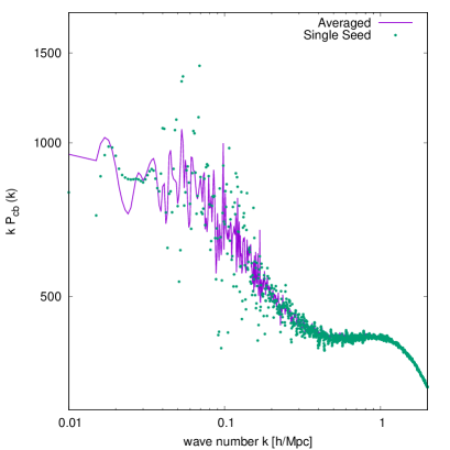
On large scales, the excellent agreement between different choices of particle number $N$ is guaranteed by the identically sized Fourier grid ($1024^{3}$ cells) used for the initialisation of all simulations, irrespective of particle numbers $N$. In this way, the smaller-$N$ runs are essentially a downsampling of the initial density field onto coarser grids, a procedure that leaves the large-scale correlations (i.e., small-$k$ power) largely unaffected between different choices of particle number $N$.

The quasi-linear and nonlinear regimes, $k\gtrsim 0.1\,h/\text{Mpc}$, however, typically become first under- and then over-powered in the low-resolution simulations. The former, under-powering phenomenon can be attributed to the finite mass resolution: the further the separation between simulation particles and the higher the mass each particle carries, the less efficiently the particles can cluster nonlinearly. The latter, over-powering effect is, on the other hand, a manifestation of Poisson noise. With a larger number of simulation particles, both of these artefacts can be pushed to a larger value of $k$. Evidently in the left panel of figure 2, percent-level agreement between the $N=512^{3}$ and $1024^{3}$ runs can be achieved up to $k\sim 2\,h/\text{Mpc}$.

The right panel of figure 2 compares the cb power spectrum extracted from a single realisation and one formed from averaging over five power spectra computed using five different sets of initial seeds. As expected, the low-$k$ region most susceptible to sample variance suffers from less scatter when averaged over five different sets of seeds. Conversely, the high-$k$ region is largely unaffected by averaging, since there is inherently enough volume here to overcome sample variance even in one single realisation.

Convergence can also be demonstrated in the relative total matter power spectrum, defined here as the power spectrum ratio of a massive neutrino cosmology to the reference $\Lambda$CDM model simulated under identical conditions, including identical initial seeds. Figure 3 shows four sets of relative total matter power spectra between the models Nu1 and Ref1, computed using four choices of particle numbers ($N=128^{3},256^{3},512^{3},1024^{3}$).

At $k\lesssim 0.1\,h/\text{Mpc}$, the relative power is consistent across all mass resolutions tested. For all four choices of $N$ we observe a spoon-like dip followed by an upturn feature, consistent with previous findings [20, 48, 30, 28]. The physical origin and nature of the spoon feature have been discussed in detail in terms of the halo model [41]. Here, we merely observe that the dip occurs at the same $k\sim 0.7\,h/{\rm Mpc}$ in all runs; the low-resolution runs tend however to predict too deep a dip followed by too high an upturn at $k\gtrsim 1\,h/\text{Mpc}$. As in figure 2, these low-resolution artefacts seen in figure 3 are a consequence first of power underestimation due to poor mass resolution and then of high-$k$ Poisson noise, both of which dominate over neutrino free-streaming effects on small scales.

On the other hand, the higher-resolution ($N=512^{3},1024^{3}$) relative power spectrum predictions exhibit sub-percent level agreement up to $k\sim 6\,h/\text{Mpc}$, exceeding the $k\sim 2\,h/\text{Mpc}$ limit on the concordant region seen in figure 2 for their absolute power spectrum counterparts. This observation is consistent with the proposition of [49], which states that the relative power spectrum generally exhibits better convergence properties than can be achieved for the absolute power spectrum using the same simulation settings.

Henceforth, unless otherwise specified, we shall always use the highest-resolution setting ($N=1024^{3},\,V=512^{3}\,(\text{Mpc}/h)^{3}$) achievable on our computing facilities in our simulations. Where comparisons are called for (e.g., between cosmological models, between methods, etc.), we always compare simulation results initialised with the same seeds.

Let us compare first our SuperEasy method with the original integral linear response approach of reference [29], which explicitly solves the integral linear response function (2.10) within the $N$-body code to obtain the neutrino density contrast at every time step. Other than this integral evaluation, the two methods share an identical perturbative starting point for the neutrino sector and evolve the cold sector in the presence of neutrino clustering in exactly the same way. The comparison is therefore largely straightforward, save for some details in the implementation of the response function (2.10) in Gadget-2, to be discussed below.

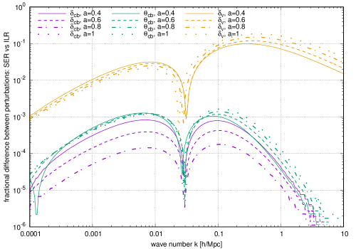
As a warm-up exercise, we first contrast the two solutions to the linearised equation of motion (4.1) for the cb density contrast ${\delta}_{\rm cb}(k)$ and velocity divergence ${\theta}_{\rm cb}(k)$, using in the gravitational potential $\phi$ the neutrino density contrast ${\delta}_{\nu}(k)$ computed from (i) the SuperEasy response function (3.18), and (ii) the full integral response function (2.10). As in the scale-back initialisation procedure, we normalise ${\delta}_{\rm cb}$ at $z=0$. Figure 4 shows the fractional differences in ${\delta}_{\rm cb}$, ${\theta}_{\rm cb}$, and ${\delta}_{\nu}$ between these approximations for the model Nu1 at a range of redshifts. Clearly, all three quantities exhibit two peaks in the intermediate $k$-region, indicating the same interpolation discrepancy previously observed in figure 1 in our comparison of the SuperEasy and class outputs. The maximum discrepancy in ${\delta}_{\nu}$ is again about 20%, while the differences in ${\delta}_{\rm cb}$ and in ${\theta}_{\rm cb}$ are at most 0.2%. The agreement in ${\delta}_{\text{cb}}$ improves with lower redshift, but this merely reflects our choice of normalisation at $z=0$.

Next, we compare the nonlinear outputs of the two methods embedded in an $N$-body simulation. To this end, we implement the integral linear response function (2.10) in Gadget-2 following reference [29]. As with SuperEasy linear response, the entry point for the implementation of integral linear response is the Fourier grid and hence the Poisson equation in the PM component. However, because the integral linear response function (2.10) involves a time-integration of the gravitational potential evolution history on each $\vec{k}$-grid point, to save computing resources reference [29] advocates (i) storing only one $\langle{\phi}(\vec{k})\rangle$ per $k\equiv|\vec{k}|$ mode averaged over all $\hat{k}$ directions, i.e., identical $|{\delta}_{\nu}(\vec{k})|$ for all vectors $\vec{k}$ with the same magnitude $k$, and (ii) the final ${\delta}_{\nu}(\vec{k})$ on a $\vec{k}$-grid point assumes the same complex phase as the cb density contrast ${\delta}_{\rm cb}(\vec{k})$ on that same $\vec{k}$-grid point. To make the comparison as direct as possible, we implement the same averaging procedure in our SuperEasy simulations, although in practice this extra step makes no more than a 0.1% difference to the final result, and, from the SuperEasy perspective, in fact detracts from the simplicity of the method.

Likewise, the Hubble expansion history and time step divisions in the execution of the simulations are kept consistent across the comparison. Initialisation of the integral linear response simulation follows the same scale-back procedure described in section 4.2, but with the neutrino density contrast ${\delta}_{\nu}(k)$ now computed from the integral linear response function (2.10) instead of the SuperEasy response function (3.18). Figure 5 shows the fractional difference between the two $z=49$ cb power spectra used to initialise the SuperEasy and the integral response linear simulations of the Nu1 model. The biggest difference shows up on the large scales around $k\sim 0.003~{}h/{\rm Mpc}$, but still remains within 0.4% agreement.

Figure 6 shows the fractional differences in the cb power spectrum and in the total matter power spectrum between the SuperEasy and integral linear response methods for the models Nu1, Nu2, and Nu3 at a range of redshifts. Evidently, the agreement between the two methods in predicting the cb power spectrum is excellent across the whole redshift range tested (0.1% or better), even for the most extreme Nu1 model. The total matter power spectrum predictions likewise agree to within sub-percent level on all scales at $z>0.5$. Unsurprisingly, interpolation error in the SuperEasy gravitational potential causes the SuperEasy power spectrum to overshoot its integral response counterpart around $k\sim 0.1\,h/\text{Mpc}$ by up to 1% at $z=0$. As the neutrinos’ contribution to nonlinear clustering diminishes with lower neutrino masses, however, the agreement between the two methods also improves.

Thus, to conclude this subsection, even in a cosmology with a neutrino mass sum as large as $\sum m_{\nu}\sim 1$ eV, SuperEasy linear response is able to match the original integral linear response method [29] to 0.1% agreement in the cb power spectrum and 1.2% agreement in the total matter power spectrum. For a lower mass sum of $\sum m_{\nu}\sim 0.5$ eV, the agreement improves to 0.05% in the cb power and 0.5% in the total matter power. For mass sums comparable to current cosmological bounds, $\sum m_{\nu}\sim 0.2$ eV, 0.1% agreement can be achieved in both the cb and the total matter power spectrum across the entire accessible $k$-range.

Next, we compare power spectrum predictions obtained from our SuperEasy linear response Gadget-2 simulations with independent calculations from reference [41] using PKDGRAV3 [50]. PKDGRAV3 is a tree code wherein the cold matter particles are evolved under gravity using a variation of the oct-tree method. Reference [41] simulated massive neutrinos by evolving linear neutrino perturbations on a grid following the method of [27]. At every time step, the neutrino contribution is interpolated to the positions of the cold matter particles for the force calculation.

Before we compare the two sets of results, we note first of all that a direct comparison of the absolute cb or total matter power spectrum outputted by different simulation codes for the same cosmology typically suffers from a $\sim 10$% systematic difference [51] on small length scales,²²2The convergence “trajectory” between different simulation codes are not expected to be the same. Where one code may overestimate power at lower resolution, another may underestimate it. In reference [51], this convergence-related disagreement occurs at very high $k$-values ($\sim$ 10 $h$/Mpc), as the simulations used in that work had excellent mass resolution. Our simulations do not have the same excellent mass resolution; the code discrepancies therefore also show up in a much lower $k$-region ($\sim$ 2 $h$/Mpc). too large for the kind of comparisons we are interested in — comparisons that concern percent-level effects — to be meaningful. Conversely, the relative power spectrum between two cosmologies computed under the same conditions and with the same simulation code generally end up quite insensitive to those exact conditions or the code with which the simulations have been performed, because by forming ratios multiplicative systematic simulation errors tend to cancel [49]. We therefore choose to compare relative power spectra.

Figure 7 shows the $z=0$ relative cb power spectrum of the Nu5 to the Nu4 model of table 1 obtained from our SuperEasy Gadget-2 simulations, alongside the same quantity formed from the PKDGRAV3 simulations of reference [41] for two equivalent massive neutrino cosmologies (labelled $\nu\Lambda$CDM5 and $\nu\Lambda$CDM4 in that work). Note that for a consistent comparison with $\nu\Lambda$CDM5 and $\nu\Lambda$CDM4, we have also simulated our models Nu4 and Nu5 using the same unequal neutrino masses.³³3The specific neutrino mass values in the $\nu\Lambda$CDM4 and $\nu\Lambda$CDM5 cosmologies of reference [41] are, respectively, $\{m_{1},m_{2},m_{3}\}=\{0,0.0087,0.05\}$ eV and $\{0,0.0087,0.15\}$ eV. See appendix A for the details on how to implement the SuperEasy linear response method in scenarios involving multiple free-streaming lengths. Evidently, the two sets of simulations generally agree very well with one another across the whole $k$-range tested. We find however the spoon ratio in the high-$k$ region ($k\gtrsim 2h/\text{Mpc}$) to be highly sensitive to the random seed used to generate a particular realisation. Averaging over multiple realisations improves the small discrepancy at $k\gtrsim 2h$/Mpc seen in figure 7.

Thus, to conclude, our implementation of SuperEasy linear response in Gadget-2 is able to accurately reproduce existing independent calculations of the relative cb power spectrum between two massive neutrino cosmologies that not only utilised a completely different modelling of the neutrino perturbations, but also a different $N$-body code. Together with the comparison with integral linear response in section 6.1, this agreement lends credence to the SuperEasy linear response method as an extremely low-cost and yet reliable way to model the effects of massive neutrinos in nonlinear large-scale structure formation.

We are interested in the deviation of the perturbed neutrino phase space density from the background distribution, $\delta f(\vec{k},\vec{p},s)\equiv f(\vec{k},\vec{p},s)-\bar{f}(p)$. This can be extracted from the perturbed part of (2.9),

$$\delta f(\vec{k},\vec{p},s)=im_{\nu}k\mu\frac{\partial\bar{f}}{\partial p}\int_{s_{\rm i}}^{s}\mathrm{d}s^{\prime}\,a^{2}(s^{\prime})\,{\phi}(k,s^{\prime})\,\text{exp}\!\left(-\frac{ikp\mu}{m_{\nu}}(s-s^{\prime})\right),$$

(7.1)

where we have defined $\mu\equiv\hat{k}\cdot\hat{p}$. To keep the calculation tractable we also assume $\phi(k,s)$ to depend only on the magnitude but not the direction of $\vec{k}$. Define the average $\langle X\rangle_{\mu}\equiv(1/2)\int_{-1}^{1}{\rm d}\mu\,X(\mu)$. Applying it to equation (7.1) we find

$$\langle\delta f\rangle_{\mu}(k,p,s)=m_{\nu}k\frac{\partial\bar{f}}{\partial p}\int_{s_{\rm i}}^{s}\mathrm{d}s^{\prime}\,a^{2}(s^{\prime})\,\phi(k,s^{\prime})\,W\left(\frac{kp(s-s^{\prime})}{m_{\nu}}\right),$$

(7.2)

with

$$W(x)\equiv\frac{\sin(x)}{x^{2}}-\frac{\cos(x)}{x}=-\frac{\mathrm{d}}{{\rm d}x}{\rm sinc}(x),$$

(7.3)

where ${\rm sinc}(x)\equiv\sin(x)/x$.

As with $\delta_{\nu}$ in section 3, equation (7.2) can be solved analytically in the clustering (small $k$) and the free-streaming (large $k$) limits. In the clustering limit, we formally set $k=0$ in the argument of the function $W$, and note that $W(x)\to x/3$ as $x\to 0$. This allows us to approximate equation (7.2) in the clustering limit as

$$\left<\delta f\right>_{\mu}^{\mathrm{C}}\simeq\frac{k^{2}}{3}\,\frac{\partial\bar{f}}{\partial\ln p}\int_{s_{\rm i}}^{s}\mathrm{d}s^{\prime}\,a^{2}(s^{\prime})\,\phi(k,s^{\prime})\,(s-s^{\prime}).$$

(7.4)

Contrasting this expression with the clustering solution (3.15) for $\delta_{\nu}$, we immediately find

$\displaystyle\langle\delta f\rangle_{\mu}^{\mathrm{C}}\simeq-\frac{1}{3}\frac{\partial\bar{f}}{\partial\ln p}\delta_{\nu}(k,s)\simeq-\frac{1}{3}\frac{\partial\bar{f}}{\partial\ln p}\delta_{\rm m}(k,s),$

(7.5)

where the second, approximate equality follows from equation (3.16).

References

- [1] Particle Data Group Collaboration, M. Tanabashi et al., “Review of Particle Physics,” Phys. Rev. D 98 (2018) no. 3, 030001.
- [2] KamLAND Collaboration, S. Abe et al., “Precision Measurement of Neutrino Oscillation Parameters with KamLAND,” Phys. Rev. Lett. 100 (2008) 221803, arXiv:0801.4589 [hep-ex].
- [3] Particle Data Group Collaboration, C. Patrignani et al., “Review of Particle Physics,” Chin. Phys. C 40 (2016) no. 10, 100001.
- [4] P. de Salas, D. Forero, C. Ternes, M. Tortola, and J. Valle, “Status of neutrino oscillations 2018: 3 hint for normal mass ordering and improved CP sensitivity,” Phys. Lett. B 782 (2018) 633–640, arXiv:1708.01186 [hep-ph].
- [5] C. Kraus et al., “Final results from phase II of the Mainz neutrino mass search in tritium beta decay,” Eur. Phys. J. C 40 (2005) 447–468, arXiv:hep-ex/0412056.
- [6] KATRIN Collaboration, A. Osipowicz et al., “KATRIN: A Next generation tritium beta decay experiment with sub-eV sensitivity for the electron neutrino mass. Letter of intent,” arXiv:hep-ex/0109033.
- [7] Project 8 Collaboration, A. Ashtari Esfahani et al., “Determining the neutrino mass with cyclotron radiation emission spectroscopy—Project 8,” J. Phys. G 44 (2017) no. 5, 054004, arXiv:1703.02037 [physics.ins-det].
- [8] J. Lesgourgues and S. Pastor, “Massive neutrinos and cosmology,” Phys. Rept. 429 (2006) 307–379, arXiv:astro-ph/0603494.
- [9] Y. Y. Wong, “Neutrino mass in cosmology: status and prospects,” Ann. Rev. Nucl. Part. Sci. 61 (2011) 69–98, arXiv:1111.1436 [astro-ph.CO].
- [10] Planck Collaboration, N. Aghanim et al., “Planck 2018 results. VI. Cosmological parameters,” arXiv:1807.06209 [astro-ph.CO].
- [11] A. Upadhye, “Neutrino mass and dark energy constraints from redshift-space distortions,” JCAP 05 (2019) 041, arXiv:1707.09354 [astro-ph.CO].
- [12] LSST Science, LSST Project Collaboration, P. A. Abell et al., “LSST Science Book, Version 2.0,” arXiv:0912.0201 [astro-ph.IM].
- [13] EUCLID Collaboration, R. Laureijs et al., “Euclid Definition Study Report,” arXiv:1110.3193 [astro-ph.CO].
- [14] CMB-S4 Collaboration, K. N. Abazajian et al., “CMB-S4 Science Book, First Edition,” arXiv:1610.02743 [astro-ph.CO].
- [15] A. Chudaykin and M. M. Ivanov, “Measuring neutrino masses with large-scale structure: Euclid forecast with controlled theoretical error,” JCAP 11 (2019) 034, arXiv:1907.06666 [astro-ph.CO].
- [16] J. Lesgourgues and S. Pastor, “Neutrino mass from Cosmology,” Adv. High Energy Phys. 2012 (2012) 608515, arXiv:1212.6154 [hep-ph].
- [17] A. Lewis, A. Challinor, and A. Lasenby, “Efficient computation of CMB anisotropies in closed FRW models,” Astrophys. J. 538 (2000) 473–476, arXiv:astro-ph/9911177.
- [18] D. Blas, J. Lesgourgues, and T. Tram, “The Cosmic Linear Anisotropy Solving System (CLASS) II: Approximation schemes,” JCAP 07 (2011) 034, arXiv:1104.2933 [astro-ph.CO].
- [19] J. Dakin, J. Brandbyge, S. Hannestad, T. Haugbølle, and T. Tram, “COCEPT: Cosmological neutrino simulations from the non-linear Boltzmann hierarchy,” JCAP 1902 (2019) 052, arXiv:1712.03944 [astro-ph.CO].
- [20] J. Brandbyge, S. Hannestad, T. Haugbølle, and B. Thomsen, “The Effect of Thermal Neutrino Motion on the Non-linear Cosmological Matter Power Spectrum,” JCAP 08 (2008) 020, arXiv:0802.3700 [astro-ph].
- [21] M. Viel, M. G. Haehnelt, and V. Springel, “The effect of neutrinos on the matter distribution as probed by the Intergalactic Medium,” JCAP 06 (2010) 015, arXiv:1003.2422 [astro-ph.CO].
- [22] F. Villaescusa-Navarro, F. Marulli, M. Viel, E. Branchini, E. Castorina, E. Sefusatti, and S. Saito, “Cosmology with massive neutrinos I: towards a realistic modeling of the relation between matter, haloes and galaxies,” JCAP 03 (2014) 011, arXiv:1311.0866 [astro-ph.CO].
- [23] J. Adamek, R. Durrer, and M. Kunz, “Relativistic N-body simulations with massive neutrinos,” JCAP 11 (2017) 004, arXiv:1707.06938 [astro-ph.CO].
- [24] A. E. Bayer, A. Banerjee, and Y. Feng, “A fast particle-mesh simulation of non-linear cosmological structure formation with massive neutrinos,” JCAP 01 (2021) 016, arXiv:2007.13394 [astro-ph.CO].
- [25] A. Banerjee, D. Powell, T. Abel, and F. Villaescusa-Navarro, “Reducing Noise in Cosmological N-body Simulations with Neutrinos,” JCAP 09 (2018) 028, arXiv:1801.03906 [astro-ph.CO].
- [26] W. Elbers, C. S. Frenk, A. Jenkins, B. Li, and S. Pascoli, “An optimal nonlinear method for simulating relic neutrinos,” arXiv:2010.07321 [astro-ph.CO].
- [27] J. Brandbyge and S. Hannestad, “Grid Based Linear Neutrino Perturbations in Cosmological N-body Simulations,” JCAP 05 (2009) 002, arXiv:0812.3149 [astro-ph].
- [28] C. Partmann, C. Fidler, C. Rampf, and O. Hahn, “Fast simulations of cosmic large-scale structure with massive neutrinos,” arXiv:2003.07387 [astro-ph.CO].
- [29] Y. Ali-Haimoud and S. Bird, “An efficient implementation of massive neutrinos in non-linear structure formation simulations,” Mon. Not. Roy. Astron. Soc. 428 (2012) 3375–3389, arXiv:1209.0461 [astro-ph.CO].
- [30] S. Bird, Y. Ali-Haïmoud, Y. Feng, and J. Liu, “An Efficient and Accurate Hybrid Method for Simulating Non-Linear Neutrino Structure,” Mon. Not. Roy. Astron. Soc. 481 (2018) no. 2, 1486–1500, arXiv:1803.09854 [astro-ph.CO].
- [31] T. Tram, J. Brandbyge, J. Dakin, and S. Hannestad, “Fully relativistic treatment of light neutrinos in -body simulations,” JCAP 03 (2019) 022, arXiv:1811.00904 [astro-ph.CO].
- [32] A. Ringwald and Y. Y. Wong, “Gravitational clustering of relic neutrinos and implications for their detection,” JCAP 12 (2004) 005, arXiv:hep-ph/0408241.
- [33] E. Lawrence, K. Heitmann, J. Kwan, A. Upadhye, D. Bingham, S. Habib, D. Higdon, A. Pope, H. Finkel, and N. Frontiere, “The Mira-Titan Universe II: Matter Power Spectrum Emulation,” Astrophys. J. 847 (2017) no. 1, 50, arXiv:1705.03388 [astro-ph.CO].
- [34] J. Z. Chen, A. Upadhye, and Y. Y. Wong, “The cosmic neutrino background as a collection of fluids,” arXiv:2011.XXXXX.
- [35] J. Brandbyge and S. Hannestad, “Resolving Cosmic Neutrino Structure: A Hybrid Neutrino N-body Scheme,” JCAP 1001 (2010) 021, arXiv:0908.1969 [astro-ph.CO].
- [36] E. Bertschinger, “Cosmological dynamics: Course 1,” in Les Houches Summer School on Cosmology and Large Scale Structure (Session 60), pp. 273–348. 8, 1993. arXiv:astro-ph/9503125.
- [37] R. H. Brandenberger, N. Kaiser, and N. Turok, “Dissipationless Clustering of Neutrinos Around a Cosmic String Loop,” Phys. Rev. D 36 (1987) 2242.
- [38] K. Abazajian, E. R. Switzer, S. Dodelson, K. Heitmann, and S. Habib, “The Nonlinear cosmological matter power spectrum with massive neutrinos. 1. The Halo model,” Phys. Rev. D 71 (2005) 043507, arXiv:astro-ph/0411552.
- [39] F. Bernardeau, S. Colombi, E. Gaztanaga, and R. Scoccimarro, “Large scale structure of the universe and cosmological perturbation theory,” Phys. Rept. 367 (2002) 1–248, arXiv:astro-ph/0112551 [astro-ph].
- [40] Y. Y. Wong, “Higher order corrections to the large scale matter power spectrum in the presence of massive neutrinos,” JCAP 10 (2008) 035, arXiv:0809.0693 [astro-ph].
- [41] S. Hannestad, A. Upadhye, and Y. Y. Wong, “Spoon or slide? The non-linear matter power spectrum in the presence of massive neutrinos,” arXiv:2006.04995 [astro-ph.CO].
- [42] A. Aviles and A. Banerjee, “A Lagrangian Perturbation Theory in the presence of massive neutrinos,” JCAP 10 (2020) 034, arXiv:2007.06508 [astro-ph.CO].
- [43] M. Garny and P. Taule, “Loop corrections to the power spectrum for massive neutrino cosmologies with full time- and scale-dependence,” arXiv:2008.00013 [astro-ph.CO].
- [44] V. Springel, “The Cosmological simulation code GADGET-2,” Mon. Not. Roy. Astron. Soc. 364 (2005) 1105–1134, arXiv:astro-ph/0505010 [astro-ph].
- [45] R. Angulo, V. Springel, S. White, A. Jenkins, C. Baugh, and C. Frenk, “Scaling relations for galaxy clusters in the Millennium-XXL simulation,” Mon. Not. Roy. Astron. Soc. 426 (2012) 2046, arXiv:1203.3216 [astro-ph.CO].
- [46] WMAP Collaboration, C. Bennett et al., “Nine-Year Wilkinson Microwave Anisotropy Probe (WMAP) Observations: Final Maps and Results,” Astrophys. J. Suppl. 208 (2013) 20, arXiv:1212.5225 [astro-ph.CO].
- [47] I. M. Oldengott, G. Barenboim, S. Kahlen, J. Salvado, and D. J. Schwarz, “How to relax the cosmological neutrino mass bound,” JCAP 04 (2019) 049, arXiv:1901.04352 [astro-ph.CO].
- [48] S. Bird, M. Viel, and M. G. Haehnelt, “Massive Neutrinos and the Non-linear Matter Power Spectrum,” Mon. Not. Roy. Astron. Soc. 420 (2012) 2551–2561, arXiv:1109.4416 [astro-ph.CO].
- [49] S. Hannestad and Y. Y. Wong, “Fitting functions on the cheap: the relative nonlinear matter power spectrum,” JCAP 03 (2020) 028, arXiv:1907.01125 [astro-ph.CO].
- [50] D. Potter, J. Stadel, and R. Teyssier, “PKDGRAV3: Beyond Trillion Particle Cosmological Simulations for the Next Era of Galaxy Surveys,” arXiv:1609.08621 [astro-ph.IM].
- [51] A. Schneider, R. Teyssier, D. Potter, J. Stadel, J. Onions, D. S. Reed, R. E. Smith, V. Springel, F. R. Pearce, and R. Scoccimarro, “Matter power spectrum and the challenge of percent accuracy,” JCAP 04 (2016) 047, arXiv:1503.05920 [astro-ph.CO].
- [52] F. Führer and Y. Y. Y. Wong, “Higher-order massive neutrino perturbations in large-scale structure,” JCAP 03 (2015) 046, arXiv:1412.2764 [astro-ph.CO].