Once is Never Enough:
Foundations for Sound Statistical Inference in Tor Network Experimentation
Abstract
Tor is a popular low-latency anonymous communication system that focuses on usability and performance: a faster network will attract more users, which in turn will improve the anonymity of everyone using the system. The standard practice for previous research attempting to enhance Tor performance is to draw conclusions from the observed results of a single simulation for standard Tor and for each research variant. But because the simulations are run in sampled Tor networks, it is possible that sampling error alone could cause the observed effects. Therefore, we call into question the practical meaning of any conclusions that are drawn without considering the statistical significance of the reported results.
In this paper, we build foundations upon which we improve the Tor experimental method. First, we present a new Tor network modeling methodology that produces more representative Tor networks as well as new and improved experimentation tools that run Tor simulations faster and at a larger scale than was previously possible. We showcase these contributions by running simulations with 6,489 relays and 792k simultaneously active users, the largest known Tor network simulations and the first at a network scale of 100%. Second, we present new statistical methodologies through which we: (i) show that running multiple simulations in independently sampled networks is necessary in order to produce informative results; and (ii) show how to use the results from multiple simulations to conduct sound statistical inference. We present a case study using 420 simulations to demonstrate how to apply our methodologies to a concrete set of Tor experiments and how to analyze the results.
1 Introduction
Tor [15] is a privacy-enhancing technology and the most popular anonymous communication system ever deployed. Tor consists of a network of relays that forward traffic on behalf of Tor users (i.e., clients) and Internet destinations. The Tor Project estimates that there are about 2M daily active Tor users [48], while recent privacy-preserving measurement studies estimate that there are about 8M daily active users [50] and 792k simultaneously active users [38]. Tor is used for a variety of reasons, including blocking trackers, defending against surveillance, resisting fingerprinting and censorship, and freely browsing the Internet [68].
The usability of the Tor network is fundamental to the security it can provide [14]; prior work has shown that real-world adversaries intentionally degrade usability to cause users to switch to less secure communication protocols [6]. Good usability enables Tor to retain more users [18], and more users generally corresponds to better anonymity [1]. Tor has made improvements in three primary usability components: (i) the design of the interface used to access and use the network (i.e., Tor Browser) has been improved through usability studies [11, 57, 45]; (ii) the performance perceived by Tor users has improved through the deployment of new traffic scheduling algorithms [37, 64]; and (iii) the network resources available for forwarding traffic has grown from about 100 Gbit/s to about 400 Gbit/s in the last 5 years [66]. Although these changes have contributed to user growth, continued growth in the Tor network is desirable—not only because user growth improves anonymity [1], but also because access to information is a universal and human right [71] and growth in Tor means more humans can safely, securely, privately, and freely access information online.
Researchers have contributed numerous proposals for improving Tor performance in order to support continued growth in the network, including those that attempt to improve Tor’s path selection [73, 41, 7, 5, 46, 13, 58, 75, 61, 24, 52, 28, 60], load balancing [31, 53, 34, 22, 40, 27], traffic admission control [2, 35, 37, 21, 23, 33, 74, 47, 16, 42], and congestion control mechanisms [4, 20]. The standard practice when proposing a new mechanism for Tor is to run a single experiment with each recommended configuration of the mechanism and a single experiment with standard Tor. Measurements of a performance metric (e.g., download time) are taken during each experiment, the empirical distributions over which are directly compared across experiments. Unfortunately, the experiments (typically simulations or emulations [62]) are done in scaled-down Tor test networks that are sampled from the state of the true network at a static point in time [32]; only a single sample is considered even though in reality the network changes over time in ways that could change the conclusions. Moreover, statistical inference techniques (e.g., repeated trials and interval estimates) are generally not applied during the analysis of results, leading to questionable conclusions. Perhaps due in part to undependable results, only a few Tor performance research proposals have been deployed over the years [37, 64] despite the abundance of available research.
Contributions
We advance the state of the art by building foundations for conducting sound Tor performance research in two major ways: (i) we design and validate Tor experimentation models and develop new and improved modeling and experimentation tools that together allow us to create and run more representative Tor test networks faster than was previously possible; and (ii) we develop statistical methodologies that enable sound statistical inference of experimentation results and demonstrate how to apply our methodologies through a case study on a concrete set of Tor experiments.
Models and Tools
In §3 we present a new Tor network modeling methodology that produces more representative Tor networks by considering the state of the network over time rather than at a static point as was previously standard [32]. We designed our modeling methodology to support the flexible generation of Tor network models with configurable network, user, traffic load, and process scale factors, supporting experiments in computing facilities with a range of available resources. We designed our modeling tools such that expensive data processing tasks need only occur once, and the result can be distributed to the Tor community and used to efficiently generate any number of network models.
In §4 we contribute new and improved experimentation tools that we optimized to enable us to run Tor experiments faster and at a larger scale than was previously possible. In particular, we describe several improvements we made to Shadow [29], the most popular and validated platform for Tor experimentation, and demonstrate how our Tor network models and improvements to Shadow increase the scalability of simulations. We showcase these contributions by running the largest known Tor simulations—full-scale Tor networks with 6,489 relays and 792k simultaneously active users. We also run smaller-scale networks of 2,000 relays and 244k users to compare to prior work: we observe a reduction in RAM usage of 1.7 TiB (64%) and a reduction in run time of 33 days, 12 hours (94%) compared to the state of the art [38].
Statistical Methodologies
In §5 we describe a methodology that enables us to conduct sound statistical inference using the results collected from scaled-down (sampled) Tor networks. We find that running multiple simulations in independently sampled networks is necessary in order to obtain statistically significant results, a methodology that has never before been implemented in Tor performance research and causes us to question the conclusions drawn in previous work (see §2.4). We describe how to use multiple networks to estimate the distribution of a random variable and compute confidence intervals over that distribution, and discuss how network sampling choices would affect the estimation.
In §6 we present a case study in order to demonstrate how to apply our modeling and statistical methodologies to conduct sound Tor performance research. We present the results from a total of 420 Tor simulations across three network scale and two traffic load factors. We find that the precision of the conclusions that can be drawn from the networks used for simulations are dependent upon the scale of those networks. Although it is possible to derive similar conclusions from networks of different scales, fewer simulations are generally required in larger-scale than smaller-scale networks to achieve a similar precision. We conclude that one simulation is never enough to achieve statistically significant results.
Availability
Through this work we have developed new modeling tools and improvements to Shadow that we have released as open-source software as part of OnionTrace v1.0.0, TorNetTools v1.1.0, TGen v1.0.0, and Shadow v1.13.2.111https://github.com/shadow/{oniontrace,tornettools,tgen,shadow} We have made these and other research artifacts publicly available.222https://neverenough-sec2021.github.io
2 Background and Related Work
We provide a brief background on Tor before describing prior work on Tor experimentation, modeling, and performance.
2.1 Tor
A primary function of the Tor network is to anonymize user traffic [15]. To accomplish this, the Tor network is composed of a set of Tor relays that forward traffic through the network on behalf of users running Tor clients. Some of the relays serve as directory authorities and are responsible for publishing a network consensus document containing relay information that is required to connect to and use the network (e.g., addresses, ports, and fingerprints of cryptographic identity keys for all relays in the network). Consensus documents also contain a weight for each relay to support a weighted path selection process that attempts to balance traffic load across relays according to relay bandwidth capacity. To use the network, clients build long-lived circuits through a telescoping path of relays: the first in the path is called the guard (i.e., entry), the last is called the exit, and the remaining are called middle relays. Once a circuit is established, the client sends commands through the circuit to the exit instructing it to open streams to Internet destinations (e.g., web servers); the request and response traffic for these streams are multiplexed over the same circuit. Another, less frequently used function of the network is to support onion services (i.e., anonymized servers) to which Tor clients can connect (anonymizing both the client and the onion service to the other).
2.2 Tor Experimentation Tools
Early Tor experimentation tools included packet-level simulators that were designed to better understand the effects of Tor incentive schemes [31, 56]. Although these simulators reproduced some of Tor’s logic, they did not actually use Tor source code and quickly became outdated and unmaintained. Recognizing the need for a more realistic Tor experimentation tool, researchers began developing tools following two main approaches: network emulation and network simulation [62].
Network Emulation
ExperimenTor [8] is a Tor experimentation testbed built on top of the ModelNet [72] network emulation platform. ExperimenTor consists of two components that generally run on independent servers (or clusters): one component runs client processes and the other runs the ModelNet core emulator that connects the processes in a virtual network topology. The performance of this architecture was improved in SNEAC [63] through the use of Linux Containers and the kernel’s network emulation module netem, while tooling and network orchestration were improved in NetMirage [70].
Network Simulation
Shadow [29] is a hybrid discrete-event network simulator that runs applications as plugins. We provide more background on Shadow in §4.1. Shadow’s original design was improved with the addition of a user-space non-preemptive thread scheduler [51], and later with a high performance dynamic loader [69]. Additional contributions have been made through several research projects [35, 37, 38], and we make further contributions that improve Shadow’s efficiency and correctness as described in §4.2.
2.3 Tor Modeling
An early approach to model the Tor network was developed for both Shadow and ExperimenTor [32]. The modeling approach produced scaled-down Tor test networks by sampling relays and their attributes from a single true Tor network consensus. As a result, the models are particularly sensitive to short-term temporal changes in the composition of the true network (e.g., those that result from natural relay churn, network attacks, or misconfigurations). The new techniques we present in §3.2 are more robust to such variation because they are designed to use Tor metrics data spanning a user-selectable time period (i.e., from any chosen set of consensus files) in order to create simulated Tor networks that are more representative of the true Tor network over time.
In previous models, the number of clients to use and their behavior profiles were unknown, so finding a suitable combination of traffic generation parameters that would yield an appropriate amount of background traffic was often a challenging and iterative process. But with the introduction of privacy-preserving measurement tools [17, 30, 49, 19] and the recent publication of Tor measurement studies [30, 38, 50], we have gained a more informed understanding of the traffic characteristics of Tor. Our new modeling techniques use Markov models informed by (privacy-preserving) statistics from true Tor traffic [38], while significantly improving experiment scalability as we demonstrate in §4.3.
2.4 Tor Performance Studies
The Tor experimentation tools and models described above have assisted researchers in exploring how changes to Tor’s path selection [73, 41, 7, 5, 46, 13, 58, 75, 61, 24, 52, 28, 60], load balancing [31, 53, 34, 22, 40, 27], traffic admission control [2, 35, 37, 21, 23, 33, 74, 47, 16, 42], congestion control [4, 20], and denial of service mechanisms [36, 26, 12, 59, 39] affect Tor performance and security [3]. The standard practice that has emerged from this work is to sample a single scaled-down Tor network model and use it to run experiments with standard Tor and each of a set of chosen configurations of the proposed performance-enhancing mechanism. Descriptive statistics or empirical distributions of the results are then compared across these experiments. Although some studies use multiple trials of each experimental configuration in the chosen sampled network [34, 40], none of them involve running experiments in multiple sampled networks, which is necessary to estimate effects on the real-world Tor network (see §5). Additionally, statistical inference techniques (e.g., interval estimates) are not applied during the analysis of the results, leading to questions about the extent to which the conclusions drawn in previous work are relevant to the real world. Our work advances the state of the art of the experimental process for Tor performance research: in §5 we describe new statistical methodologies that enable researchers to conduct sound statistical inference from Tor experimentation results, and in §6 we present a case study to demonstrate how to put our methods into practice.
3 Models for Tor Experimentation
In order to conduct Tor experiments that produce meaningful results, we must have network and traffic models that accurately represent the composition and traffic characteristics of the Tor network. In this section, we describe new modeling techniques that make use of the latest data from recent privacy-preserving measurement studies [38, 50, 30]. Note that while exploring alternatives for every modeling choice that will be described in this section is out of scope for this paper, we will discuss some alternatives that are worth considering in §7.
3.1 Internet Model
Network communication is vital to distributed systems; the bandwidth and the network latency between nodes are primary characteristics that affect performance. Jansen et al. have produced an Internet map [38] that we find useful for our purposes; we briefly describe how it was constructed before explaining how we modify it.
To produce an Internet map, Jansen et al. [38] conducted Internet measurements using globally distributed vantage points (called probes) from the RIPE Atlas measurement system (atlas.ripe.net). They assigned a representative probe for each of the 1,813 cities in which at least one probe was available. They used ping to estimate the latency between all of the 1,642,578 distinct pairs of representative probes, and they crawled speedtest.net to extract upstream and downstream bandwidths for each city.333speedtest.net ranks mobile and fixed broadband speeds around the world. They encoded the results into an Internet map stored in the graphml file format; each vertex corresponds to a representative probe and encodes the bandwidth available in that city, and each edge corresponds to a path between a pair of representative probes and encodes the network latency between the pair.
Also encoded on edges in the Internet map were packet loss rates. Each edge was assigned a packet loss rate according to the formula where is the latency of edge . This improvised formula was not based on any real data. Our experimentation platform (described in §4) already includes for each host an edge router component that drops packets when buffers are full. Because additional packet loss from core routers is uncommon [44], we modify the Internet map by setting to zero for all edges.444Future work should consider developing a more realistic packet loss model that is, e.g., based on measurements of actual Tor clients and relays. We use the resulting Internet model in all simulations in this paper.
3.2 Tor Network Model
To the Internet model we add hosts that run Tor relays and form a Tor overlay network. The Tor modeling task is to choose host bandwidths, Internet locations, and relay configurations that support the creation of Tor test networks that are representative of the true Tor network.
We construct Tor network models in two phases: staging and generation. The two-phase process allows us to perform the computationally expensive staging phase once, and then perform the computationally inexpensive generation phase any number of times. It also allows us to release the staging files to the community, whose members may then use our Tor modeling tools without first processing large datasets.
| Stat. | Description |
| the fraction of consensuses in which relay was running | |
| the fraction of consensuses in which relay was a guard | |
| the fraction of consensuses in which relay was an exit | |
| the median normalized consensus weight of relay | |
| the max observed bandwidth of relay | |
| the median bandwidth rate of relay | |
| the median bandwidth burst of relay | |
| median across consensuses of relay count for each position | |
| median across consensuses of total weight for position | |
| median normalized probability that a user is in country |
-
Valid positions are : exit+guard, : exit, : guard, and : middle.
-
Valid countries are any two-letter country code (e.g., , , etc.).
3.2.1 Staging
Ground truth details about the temporal composition and state of the Tor network are available in Tor network data files (i.e., hourly network consensus and daily relay server descriptor files) which have been published since 2007. We first gather the subset of these files that represents the time period that we want to model (e.g., all files published in January 2019), and then extract network attributes from the files in the staging phase so that we can make use of them in the networks we later generate. In addition to extracting the IP address, country code, and fingerprint of each relay , we compute the per-relay and network summary statistics shown in Table 1. We also process the Tor users dataset containing per-country user counts, which Tor has published daily since 2011 [66]. From this data we compute the median normalized probability that a user appears in each country. We store the results of the staging phase in two small JSON files (a few MiB each) that we use in the generation phase. Note that we could make use of other network information if it were able to be safely measured and published (see Appendix A for an ontology of some independent variables that could be useful).
3.2.2 Generation
In the generation phase, we use the data extracted during the staging phase and the results from a recent privacy-preserving Tor measurement study [38] to generate Tor network models of a configurable scale. For example, a 100% Tor network represents a model of equal scale to the true Tor network. Each generated model is stored in an XML configuration file, which specifies the hosts that should be instantiated, their bandwidth properties and locations in the Internet map, the processes they run, and configuration options for each process. Instantiating a model will result in a Tor test network that is representative of the true Tor network. We describe the generation of the configuration file by the type of hosts that make up the model: Tor network relays, traffic generation, and performance benchmarking.
Tor Network Relays
The relay staging file may contain more relays than we need for a 100% Tor network (due to relay churn in the network during the staged time period), so we first choose enough relays for a 100% Tor network by sampling relays without replacement, using each relay’s running frequency as its sampling weight.555Alternatives to weighted sampling should be considered if staging time periods during which the Tor network composition is extremely variable. We then assign the guard and exit flag to each of the sampled relays with a probability equal to the fraction of consensuses in which relay served as a guard and exit , respectively.
To create a network whose scale is times the size of the 100% network,666Because of the RAM and CPU requirements (see §4), we expect that it will generally be infeasible to run 100% Tor networks. The configurable scale allows for tuning the amount of resources required to run a model. we further subsample from the sampled set of relays to use in our scaled-down network model. We describe our subsampling procedure for middle relays for ease of exposition, but the same procedure is repeated for the remaining positions (see Table 1 note†). To subsample middle relays, we: (i) sort the list of sampled middle relays by their normalized consensus weight , (ii) split the list into buckets, each of which contains as close as possible to an equal number of relays, and (iii) from each bucket, select the relay with the median weight among those in the bucket. This strategy guarantees that the weight distribution across relays in our subsample is a best fit to the weight distribution of relays in the original sample [32].
A new host is added to the configuration file for each subsampled relay . Each host is assigned the IP address and country code recorded in the staging file for relay , which will allow it to be placed in the nearest city in the Internet map. The host running relay is also assigned a symmetric bandwidth capacity equal to ; i.e., we use the maximum observed bandwidth as our best estimate of a relay’s bandwidth capacity. Each host is configured to run a Tor relay process that will receive the exit and guard flags that we assigned (as previously discussed), and each relay sets its token bucket rate and burst options to and , respectively. When executed, the relay processes will form a functional Tor overlay network capable of forwarding user traffic.
Traffic Generation
A primary function of the Tor network is to forward traffic on behalf of users. To accurately characterize Tor network usage, we use the following measurements from a recent privacy-preserving Tor measurement study [38]: the total number of active users k (counted at guards) and the total number of active circuits M (counted at exits) in an average 10 minute period.
To generate a Tor network whose scale is times the size of the 100% network, we compute the total number of users we need to model as . We compute the total number of circuits that those users create every 10 minutes as , where is a load factor that allows for configuration of the amount of traffic load generated by the users ( results in “normal” traffic load). We use a process scale factor to allow for configuration of the number of Tor client processes that will be used to generate traffic on the circuits from the users. Each of Tor client processes will support the combined traffic of users, i.e., the traffic from circuits.
The factor can be used to significantly reduce the amount of RAM and CPU resources required to run our Tor model; e.g., setting means we only need to run half as many Tor client processes as the number of users we are simulating.777A primary effect of is fewer network descriptor fetches, the network impact of which is negligible relative to the total traffic generated. At the same time, is a reciprocal factor w.r.t. the traffic that each Tor client generates; e.g., setting causes each client to produce twice as many circuits (and the associated traffic) as a single user would.
We add new traffic generation client hosts to our configuration file. For each such client, we choose a country according to the probability distribution , and assign the client to a random city in that country using the Internet map in §3.1.888Shadow will arbitrarily choose an IP address for the host such that it can route packets to all other simulation hosts (clients, relays, and servers). Each client runs a Tor process in client mode configured to disable guards999Although a Tor client uses guards by default, for us it would lead to inaccurate load balancing because each client simulates users. Support in the Tor client for running multiple () parallel guard “sessions” (i.e., assigning a guard to each user “session”) is an opportunity for future work. and a TGen traffic generation process that is configured to send its traffic through the Tor client process over localhost (we significantly extend a previous version of TGen [38, §5.1] to support our models). Each TGen process is configured to generate traffic using Markov models (as we describe below), and we assign each host a bandwidth capacity equal to the maximum of Mbit/s and 1 Gbit/s to prevent it from biasing the traffic rates dictated by the Markov models when generating the combined traffic of users. Server-side counterparts to the TGen processes are also added to the configuration file (on independent hosts).
Each TGen process uses three Markov models to accurately model Tor traffic characteristics: (i) a circuit model, which captures the circuit inter-arrival process on a per-user basis; (ii) a stream model, which captures the stream inter-arrival process on a per-circuit basis; and (iii) a packet model, which captures the packet inter-arrival process on a per-stream basis. Each of these models are based on a recent privacy-preserving measurement study that used PrivCount [30] to collect measurements of real traffic being forwarded by a set of Tor exit relays [38]. We encode the circuit inter-arrival process as a simple single state Markov model that emits new circuit events according to an exponential distribution with rate microseconds, where is the number of microseconds in 10 minutes. New streams on each circuit and packets on each stream are generated using the stream and packet Markov models, respectively, which were directly measured in Tor and published in previous work [38, §5.2.3].
The rates and patterns of the traffic generated using the Markov models will mimic the rates and patterns of real Tor users: the models encode common distributions (e.g., exponential and log-normal) and their parameters, such that they can be queried to determine the amount of time to wait between the creation of new circuits and streams and the transfer of packets (in both the send and receive directions).
Each TGen client uses unique seeds for all Markov models so that it generates unique traffic characteristics.101010The Markov model seeds are unique across clients, but generated from the same master seed in order to maintain a deterministic simulation. Each TGen client also creates a unique SOCKS username and password for each generated circuit and uses it for all Tor streams generated in the circuit; due to Tor’s IsolateSOCKSAuth feature, this ensures that streams from different circuits will in fact be assigned to independent circuits.
We highlight that although prior work also made use of the stream and packet Markov models [38, §5.2.3], we extend previous work with a circuit Markov model that can be used to continuously generate circuits independent of the length of an experiment. Moreover, previous work did not consider either load scale or process scale ; allows for research under varying levels of congestion, and our optimization of simulating users in each Tor client process allows us to more quickly run significantly larger network models than we otherwise could (as we will show in §4.3).
Performance Benchmarking
The Tor Project has published performance benchmarks since 2009 [66]. The benchmark process downloads 50 KiB, 1 MiB, and 5 MiB files through the Tor network several times per hour, and records various statistics about each download including the time to download the first and last byte of the files. We mirror this process in our models; running several benchmarking clients that use some of the same code as Tor’s benchmarking clients (i.e., TGen) allows us to directly compare the performance obtained in our simulated Tor networks with that of the true Tor network.
3.2.3 Modeling Tools
We implemented several tools that we believe are fundamental to our ability to model and execute realistic Tor test networks. We have released these tools as open source software to help facilitate Tor research: (i) a new Tor network modeling toolkit called TorNetTools (3,034 LoC) that implements our modeling algorithms from §3.2.2; (ii) extensions and enhancements to the TGen traffic generator [38, §5.1] (6,531 LoC added/modified and 1,411 removed) to support our traffic generation models; and (iii) a new tool called OnionTrace (2,594 LoC) to interact with a Tor process and improve reproducibility of experiments. We present additional details about these tools in Appendix B.
4 Tor Experimentation Platform
The models that we described in §3 could reasonably be instantiated in a diverse set of experimentation platforms in order to produce representative Tor test networks. We use Shadow [29], the most popular and validated platform for Tor experimentation. We provide a brief background on Shadow’s design, explain the improvements we made to support accurate experimentation, and show how our improvements and models from §3 contribute to the state of the art.
4.1 Shadow Background
Shadow is a hybrid experimentation platform [29]. At its core, Shadow is a conservative-time discrete-event network simulator: it simulates hosts, processes, threads, TCP and UDP, routing, and other kernel operations. One of Shadow’s advantages is that it dynamically loads real applications as plugins and directly executes them as native code. In this regard, Shadow emulates a network and a Linux environment: applications running as plugins should function as they would if they were executed on a bare-metal Linux installation.
Because Shadow is a user-space, single process application, it can easily run on laptops, desktops, and servers with minimal configuration (resource requirements depend on the size of the experiment model). As a simulator, Shadow has complete control over simulated time; experiments may run faster or slower than real time depending on: (i) the simulation load relative to the processing resources available on the host machine, and (ii) the inherent parallelizability of the experiment model. This control over time decouples the fidelity of the experiment from the processing time required to execute it, and allows Shadow to scale independently of the processing capabilities of the host machine; Shadow is usually limited by the RAM requirements of its loaded plugins.
Shadow has numerous features that allow it to achieve its goals, including dynamic loading of independent namespaces for plugins [69], support for multi-threaded plugins via a non-preemptive concurrent thread scheduling library (GNU Portable Threads111111https://www.gnu.org/software/pth) [51], function interposition, and an event scheduler based on work stealing [9]. The combination of its features makes Shadow a powerful tool for Tor experimentation, and has led it to become the most popular and standard tool for conducting Tor performance research [62].
4.2 Shadow Improvements
After investigation of the results from some early experiments, we made several improvements to Shadow that we believe cause it to produce significantly more accurate results when running our Tor network models from §3.2. Our improvements include run-time optimizations, fixes to ensure deterministic execution, faster Tor network bootstrapping, more realistic TCP connection limits, and several network stack improvements (see Appendix C for more details). Our improvements have been incorporated into Shadow v1.13.2.
4.3 Evaluation
We have thus far made two types of foundational contributions: those that result in more representative Tor networks, and those that allow us to run more scalable simulations faster than was previously possible. We demonstrate these contributions through Tor network simulations in Shadow.

Representative Networks
We produce more representative networks by considering the state of the network over time rather than modeling a single snapshot as did previous work [32, 38]. We consider relay churn to demonstrate how the true Tor network changes over time. Figure 1 shows the rate of relay churn over all 744 consensus files (1 per hour) in Tor during January 2019. After 2 weeks, fewer than 75% of relays that were part of the network on 2019-01-01 still remain while more than 3,000 new relays joined the network. After 3 weeks, more new relays had joined the network than had remained since 2019-01-01. Our models account for churn by sampling from all such relays as described in §3.2.
In addition to producing more representative models, our Shadow network stack enhancements further improve network accuracy. To demonstrate these contributions, we simulate ten Tor network models that were generated following the methods in §3.2 (using Tor network state from 2019-01). We model Tor at the same scale that was used in previous work [38] (i.e., 2k relays and 250k users) using a process scale factor of (i.e., each TGen process simulated Tor users). We compare our simulation results to those produced by state-of-the-art methods [38] (which used Tor network state from 2018-01) and to reproducible Tor metrics [66, 67] from the corresponding modeling years (2019 for our work, 2018 for the CCS 2018 work).121212Although the models used Tor data spanning one month, we consider it reasonable to reflect the general state of Tor throughout the respective year.


The results in Figure 2 generally show that previous work is noticeably less accurate when compared to Tor 2018 than our work is compared to Tor 2019. We notice that previous work exhibited a high client download error rate in Figure 2(c) and significantly longer download times in Figures 2(e)–2(g) despite the network being appropriately loaded as shown in Figure 2(h). We attribute these errors to the connection limit and network stack limitations that were present in the CCS 2018 version of Shadow (the errors are not present in this work due to our Shadow improvements from §4.2). Also, we remark that the relay goodput in Figure 2(h) exhibits more variance in Tor than in Shadow because the Tor data is being aggregated over a longer time period (1 year for Tor vs. less than 1 hour for Shadow) during which the Tor network composition is significantly changing (see Figure 1).


| Model | Scale | RAM | Bootstrap Time | Total Time | |
| CCS’18 [38]† | 31% | 2.6 TiB | 3 days, 11 hrs. | 35 days, 14 hrs. | 1850 |
| This work† | 31% | 932 GiB | 17 hrs. | 2 days, 2 hrs. | 79 |
| This work‡ | 100% | 3.9 TiB | 2 days, 21 hrs. | 8 days, 6 hrs. | 310 |
-
31%: 2k relays and 250k users; 100%: 6,489 relays and 792k users
-
: ratio of real time / simulated time in steady state (after bootstrapping)
-
Using 810-core Intel Xeon E7-8891v2 CPUs each running @3.2 GHz.
-
Using 818-core Intel Xeon E7-8860v4 CPUs each running @2.2 GHz.
Scalable Simulations
Our new models and Shadow enhancements enable researchers to run larger networks faster than was previously possible. We demonstrate our improvements to scalability in two ways. First, we compare in the top part of Table 2 the resources required for the 31% experiments described above. We distinguish total run time from the time required to bootstrap all Tor relays and clients, initialize all traffic generators, and reach steady state. We reduced the time required to execute the bootstrapping process by 2 days, 18 hours, or 80%, while we reduced the total time required to run the bootstrapping process plus 25 simulated minutes of steady state by 33 days, 12 hours, or 94%. The ratio of real time units required to execute each simulated time unit during steady state (i.e., after bootstrapping has completed) was reduced by 96%, further highlighting our achieved speedup. When compared to models of the same scale from previous work, we observed that our improvements reduced the maximum RAM required to run bootstrapping plus 25 simulated minutes of steady state from 2.6 TiB down to 932 GiB (a total reduction of 1.7 TiB, or 64%).
Second, we demonstrate how our improvements enable us to run significantly larger models by running three Tor models at scale , i.e., at 100% of the size of the true Tor network. We are the first to simulate Tor test networks of this scale.131313We attempted to run a 100% scale Tor network using the CCS 2018 model [38], but it did not complete the bootstrapping phase within 30 days. The bottom part of Table 2 shows that each of our 100% Tor networks consumed at most 3.9 TiB of RAM, completed bootstrapping in 2 days, 21 hours, and ran the entire simulation (bootstrapping plus 25 simulated minutes of steady state) in 8 days, 6 hours. We show in Figure 3 that our 100% networks also achieve similar performance compared to the metrics published by Tor [67]. Our results are plotted with 95% confidence intervals to better understand how well our sampling methods are capable of reproducing the performance characteristics of the true Tor network. We describe how to conduct such a statistical inference in §5 next.
5 On the Statistical Significance of Results
Recall that our modeling methodology from §3.2 produces sampled Tor networks at scales of times the size of a 100% network. Because these networks are sampled using data from the true Tor network, there is an associated sampling error that must be quantified when making predictions about how the effects observed in sampled Tor networks generalize to the true Tor network. In this section, we establish a methodology for employing statistical inference to quantify the sampling error and make useful predictions from sampled networks. In our methodology, we: (i) use repeated sampling to generate multiple sampled Tor networks; (ii) estimate the true distribution of a random variable under study through measurements collected from multiple sampled network simulations; and (iii) compute statistical confidence intervals to define the precision of the estimation.
We remark that it is paramount to conduct a statistical inference when running experiments in sampled Tor networks in order to contextualize the results they generate. Our methodology employs confidence intervals (CIs) to establish the precision of estimations that are made across sampled networks. CIs will allow a researcher to make a statistical argument about the extent to which the results they have obtained are relevant to the real world. As we will demonstrate in §6, CIs help guide researchers to sample additional Tor networks (and run additional simulations) if necessary for drawing a particular conclusion in their research. Our methodology represents a shift in the state of the art of analysis methods typically used in Tor network performance research, which has previously ignored statistical inference and CIs altogether (see §2.4).
5.1 Methodology
When conducting research using experimental Tor networks, suppose we have an interest in a particular network metric; for example, our research might call for a focus on the distribution of time to last byte across all files of a given size downloaded through Tor as an indication of Tor performance (see our ontology in Appendix A for examples of other useful metrics). Because the values of such a variable are determined by the outcomes of statistical experiments, we refer to the variable as random variable . The true probability distribution over is , the true cumulative distribution is , and the true inverse distribution at quantile is such that . Our goal is to estimate (or equivalently, and ), which we do by running many simulations in sampled Tor networks and averaging the empirical distributions of at a number of quantiles across these simulations. Table 3 summarizes the symbols that we use to describe our methodology.
Repeated Sampling
A single network sampled from the true Tor network may not consistently produce perfectly representative results due to the sampling error introduced in the model sampling process (i.e., §3). Similarly, a single simulation may not perfectly represent a sampled network due to the sampling error introduced by the random choices made in the simulator (e.g., guard selection). Multiple samples of each are needed to conduct a statistical inference and understand the error in these sampling processes.
| Symbol | Description |
| true probability distribution of random variable | |
| cumulative distribution function of at such that | |
| inverse distribution function of at such that | |
| estimate of inverse distribution function at quantile | |
| error on inverse distribution estimate at quantile | |
| number of independently sampled Tor networks | |
| probability distribution over in network | |
| cumulative distribution function of at such that | |
| inverse distribution function of in network at quantile | |
| estimate of inverse distribution function in network at quantile | |
| error on inverse distribution estimate in network at quantile | |
| number of simulations in sampled Tor network | |
| number of samples of collected from sim in net | |
| empirical distribution over samples of from sim in net | |
| cumulative distribution function of at such that | |
| inverse distribution function of from sim in net at quantile |
We independently sample Tor networks according to §3.2. The th resulting Tor network is associated with a probability distribution which is specific to the th network and the relays that were chosen when generating it. To estimate , we run simulations in the th Tor network. During the th simulation in the th network, we sample values of from (i.e., we collect time to last byte measurements from the simulation). These samples form the empirical distribution , and we have such distributions in total (one for each simulation).
Estimating Distributions
Once we have completed the simulations and collected the empirical distributions, we then estimate the inverse distributions and associated with the sampled network and true probability distributions and , respectively.
First, we estimate each at quantile by taking the mean over the empirical distributions from network :
| (1) |
We refer to as an estimator of ; when taken over a range of quantiles, it allows us to estimate the cumulative distribution .
Second, we similarly estimate over all networks by taking the mean over the distributions estimated above:
| (2) |
We refer to as an estimator of ; when taken over a range of quantiles, it allows us to estimate the cumulative distribution .
We visualize the process of estimating in Figure 4 using an example: Figure 4(a) shows synthetic distributions where the upward arrows point to the values from network at quantile , and Figure 4(b) shows the mean of those values as the estimator . The example applies analogously when estimating each .


Computing Confidence Intervals
We quantify the precision of our estimator using CIs. To compute the CIs, we first quantify the measurement error associated with the empirical samples. This will often be negligible, but a possible source of nontrivial measurement error is resolution error; that is, if the empirical results are reported to a resolution of (e.g., 0.01 s), the resolution error for each sample will be , and the resolution error for the empirical mean of network at quantile is . Next, we quantify the sampling error associated with the estimates from Equations 1 and 2. The error associated with for network at quantile is:
| (3) |
where is the standard deviation over the empirical values at quantile (including the measurement error) and is the -value from the Student’s -distribution at confidence level with degrees of freedom [25, §10.5.1]. accounts for the sampling error and estimated true variance of the underlying distribution at . The error associated with at quantile is:
| (4) |
where is the standard deviation over the estimated inverse distribution values at quantile , and is the mean error from over all sampled networks. accounts for the sampling error introduced in the Tor network model generation and in the simulations. We can then define the CI at quantile as the interval that contains the true value from the inverse distribution with probability :
| (5) |
The width of the interval is , which we visualize at with the downward arrows and over all quantiles with the shaded region in Figure 4(b).
5.2 Discussion
Number of Samples Per Simulation
Recall that we collect empirical samples of the random variable from simulation in network . If we increase (e.g., by running the simulation for a longer period of time), this will result in a “tighter” empirical distribution that will more closely resemble the probability distribution . However, from Equation 1 we can see that only contributes a single value to the computation of for each quantile. Therefore, once we have enough samples so that reasonably approximates , it is more useful to run new simulations than to gather additional samples from the same simulation.
Number of Simulations Per Network
Additional simulations in network will provide us with additional empirical distributions , which will enable us to obtain a better estimate of . Moreover, it will also increase the precision of the CI by reducing in Equation 3: increasing the number of values at each quantile will decrease the standard deviation (if the values are normally distributed) and the -value (by increasing the number of degrees of freedom) while increasing the square root component (in the denominator of ).

Number of Sampled Networks
Additional simulations in independently sampled Tor networks will provide us with additional estimated distributions, which will enable us to obtain a better estimate of . Similarly as above, additional estimates will increase CI precision by reducing in Equation 4: the standard deviation and the -value will decrease while the square root component will increase.
To give a concrete example, suppose is normally distributed according to . The width of the resulting CI for each number of sampled networks at quantiles (i.e., P50, P90, and P99, respectively) is shown in Figure 5. Notice that the y-axis is drawn at log-scale, and shows that the width of the CI can be significantly reduced by more than an order of magnitude after running experiments in even just a small number of sampled networks. Additionally, we can see that the main improvement in confidence results from the first ten or so sampled networks, after which we observe relatively diminishing returns.
Scale
Another important factor to consider is the network scale . Larger scales (closer to 1) cause the probability distribution of each sampled network to cluster more closely around the true probability distribution , while smaller values cause the to vary more widely. Larger scales therefore induce smaller values of and therefore . (See §6.3 for a demonstration of this phenomenon.)

Sampling Error in Shadow
While includes the error due to sampling a scaled-down Tor network (i.e., §3), the main error that is accounted for in is the sampling error introduced by the choices made in the simulator. If this error is low, running additional simulations in the same network will have a reduced effect. To check the sampling error introduced by Shadow, we ran 9 simulations (3 simulations in each of 3 independently sampled networks of scale ) with unique simulator seeds. Figure 6 shows that the empirical distributions of the 50 KiB download times vary much more widely across sampled Tor networks than they do across simulations in the same network. Although it is ideal to run multiple simulations in each of multiple sampled networks, our results indicate that it may be a better use of resources to run every simulation in an independently sampled network. We believe this to be a reasonable optimization if a lack of available computational resources is a concern.
Conclusions
We have established a methodology for estimating the true distribution of random variables being studied across simulations in multiple Tor networks. Importantly, our methodology includes the computation of CIs that help researchers make statistical arguments about the conclusions they draw from Tor experiments. As we explained above and demonstrated in Figure 5, running simulations in smaller-scale Tor networks or in a smaller number of Tor networks for a particular configuration leads to larger CIs that limit us to drawing weaker conclusions from the results. Unfortunately, previous Tor research that utilizes Tor networks has focused exclusively on single Tor networks while completely ignoring CIs, leading to questionable conclusions (see §2.4).We argue that our methodology is superior to the state-of-the-art methods, and present in §6 a case study demonstrating how to put our methods into practice while conducting Tor research.
6 Case Study: Tor Usage and Performance
This section presents a case study on the effects of an increase in Tor usage on Tor client performance. Our primary goal is to demonstrate how to apply the methodologies we presented throughout this paper through a concrete set of experiments.
6.1 Motivation and Overview
Growing the Tor network is desirable because it improves anonymity [1] and access to information online [71]. One strategy for facilitating wider adoption of Tor is to deploy it in more commonly used browsers. Brave now prominently advertises on its website Tor integration into its browser’s private browsing mode, giving users the option to open a privacy-enhanced tab that routes traffic through Tor [10], and Mozilla is also interested in providing a similar “Super Private Browsing” mode for Firefox users [54]. However, Tor has never been deployed at the scale of popular browser deployments (Firefox has >250M monthly active users [55]), and many important research problems must be considered before such a deployment could occur [65]. For example, deploying Tor more widely could add enough load to the network that it reduces performance to the extent that some users are dissuaded from using it [18] while reducing anonymity for those that remain [1].
There has been little work in understanding the performance effects of increasing Tor network load as representative of the significant change in Tor usage that would likely occur in a wider deployment. Previous work that considered variable load did so primarily to showcase a new simulation tool [29] or to inform the design of a particular performance-enhancing algorithm [37, 33] rather than for the purpose of understanding network growth and scalability [43]. Moreover, previous studies of the effects of load on performance lack analyses of the statistical significance of the reported results, raising questions as to their practical meaning.
Guided by the foundations that we set out in this paper, we explore the performance effects of a sudden rise in Tor usage that could result from, e.g., a Mozilla deployment of Tor. In particular, we demonstrate the use of our methodologies with an example study of this simple hypothesis: increasing the total user traffic load in Tor by 20% will reduce the performance of existing clients by increasing their download times and download error rates. To study this hypothesis, we conduct a total of 420 simulations in independently sampled Tor networks across three network scale factors and two traffic load factors; we measure relevant performance properties and conduct a statistical analysis of the results following our methodology in §5. Our study demonstrates how to use our contributions to conduct statistically valid Tor performance research.
6.2 Experiment Setup
Experiments and Simulations
We refer to an experiment as a unique pair of network scale and load configurations, and a simulation as a particular execution of an experiment configuration. We study our hypothesis with a set of 6 experiments; for each experiment, we run multiple simulations in independent Tor networks so that we can quantify the statistical significance of the results following our guidance from §5.
Tor Network Scale and Load
The Tor network scales that a researcher can consider are typically dependent on the amount of RAM to which they have access. Although we were able to run a 100% Tor network for our evaluation in §4, we do not expect that access to a machine with 4 TiB of RAM, as was required to run the simulation, will be common. Because it will be more informative, we focus our study on multiple smaller network scales with more accessible resource requirements while showing the change in confidence that results from running networks of different scales. In particular, our study considers Tor network scales of 1%, 10%, and 30% () of the size of the true Tor network. At each of these network scales, we study the performance effects of 100% and 120% traffic load () using a process scale factor of , i.e., each TGen process simulates Tor users.
| Scale | Load | Sims | CPU⋆ | RAM/Sim† | Run Time/Sim‡ |
| 1% | 100% | 100 | 48 | 35 GiB | 4.8 hours |
| 1% | 120% | 100 | 48 | 50 GiB | 6.7 hours |
| 10% | 100% | 100 | 48 | 355 GiB | 19.4 hours |
| 10% | 120% | 100 | 48 | 416 GiB | 23.4 hours |
| 30% | 100% | 10 | 88 | 1.07 TiB | 4 days, 21 hours |
| 30% | 120% | 10 | 88 | 1.25 TiB | 5 days, 22 hours |
-
48-core Intel Xeon E5 @3.3 GHz; 88-core Intel Xeon E5 @2.7 GHz.
-
The median of the per-simulation max RAM usage over all simulations.
-
The median of the per-simulation run time over all simulations.
Number of Simulations
Another important consideration in our evaluation is the number of simulations to run for each experiment. As explained in §5, running too few simulations will result in wider confidence intervals that will limit us to weaker conclusions. The number of simulations that should be run typically depends on the results and the arguments being made, but in our case we run more than we require to validate our hypothesis in order to demonstrate the effects of varying . As shown in the left part of Table 4, we run a total of 420 simulations across our 6 experiments (three network scales and two load factors) using two machine profiles: one profile included 48-core Intel Xeon E5-4627 CPUs running at a max clock speed of 3.3 GHz and 1.25 TiB of RAM; the other included 88-core Intel Xeon E5-4650 CPUs running at a max clock speed of 2.7 GHz and 1.5 TiB of RAM.
| Scale | DirAuth | Guard | Middle | Exit | E+G† | Markov | Perf‡ | Server |
| 1% | 3 | 20 | 36 | 4 | 4 | 100 | 8 | 10 |
| 10% | 3 | 204 | 361 | 40 | 44 | 792 | 79 | 79 |
| 30% | 3 | 612 | 1,086 | 118 | 129 | 2,376 | 238 | 238 |
-
Total number of relays at =1%: 67; at =10%: 652; and at =30%: 1,948.
-
E+G: Relays with both the exit and guard flags ‡ Perf: Benchmark clients


Simulation Configuration
We run each simulation using an independently sampled Tor network in order to ensure that we produce informative samples following our guidance from §5. Each Tor network is generated following our methodology from §3 using the parameter values described above and Tor network state files from January 2019. The resulting network composition for each scale is shown in Table 5.
Each simulation was configured to run for 1 simulated hour. The relays bootstrapped a Tor overlay network within the first 5 minutes; all of the TGen clients and servers started their traffic generation process within 10 simulated minutes of the start of each simulation. TGen streams created by Markov clients were set to time out if no bytes were transferred in any contiguous 5 simulated minute period (the default apache client timeout), or if the streams were not complete within an absolute time of 10 simulated minutes. Timeouts for streams created by benchmarking clients were set to 15, 60, and 120 seconds for 50 KiB, 1 MiB, and 5 MiB transfers, respectively.
6.3 Results
During each simulation, we measure and collect the properties that allow us to understand our hypothesis. Ultimately, we would like to test if increasing the traffic load on the network by 20% (from to ) will reduce client performance. Therefore, we focus this study on client download time and download error rates while noting that it will very likely be useful to consider additional properties when studying more complex hypotheses (see Appendix A).
For each experiment, we combine the results from the simulations141414We ignore the results from the first 20 simulated minutes of each simulation to allow time for the network to bootstrap and reach a steady state. following the methodology outlined in §5 and present the estimated true cumulative distributions with the associated CIs (as in Figure 4) at confidence. We plot the results for varying values of as overlapping intervals (the CIs tighten as increases) for instructional purposes. Finally, we compare our results across network scales to highlight the effect of scale on the confidence in the results.


Client Download Time
The time it takes to download a certain number of bytes through Tor (i.e., the time to first/last byte) allows us to assess and compare the overall performance that a Tor client experiences. We measure download times for the performance benchmarking clients throughout the simulations. We present in Figure 7 the time to last byte for 1 MiB file downloads, while noting that we find similar trends for other file download sizes as shown in Figures 9, 10, and 11 in Appendix D. The CDFs are plotted with tail-logarithmic y-axes in order to highlight the long tail of network performance as is typically used as an indication of usability.
Figure 7(a) shows the result of our statistical analysis from §5 when using a network scale of 1% (). Against our expectation, our estimates of the true CDFs (i.e., the solid lines) indicate that the time to download 1 MiB files actually decreased after we increased the traffic load by 20%. However, notice the extent to which the confidence intervals overlap: for example, the width of the region of overlap of the and CIs is about 20 seconds at P90 (i.e., at seconds) when , and is about 3 seconds at P90 (i.e., at seconds) when . Importantly, the estimated true CDF for falls completely within the CIs for and the estimated true CDF for falls completely within the CIs for , even when considering simulations for each experiment. Therefore, it is possible that the position of the true CDFs could actually be swapped compared to what is shown in Figure 7(a). If we had followed previous work and ignored the CIs, it would have been very difficult to notice this statistical possibility. Based on these results alone, we are unable to draw conclusions about our hypothesis at the desired confidence.
Our experiments with the network scale of 10% offer more reliable results. Figure 7(b) shows the extent to which the CIs become narrower as increases from 5 to 10 to 100. Although there is some overlap in the and CIs at some values when is either 5 or 10, we can confidently confirm our hypothesis when because the estimated true CDFs and their CIs are completely distinguishable. Notice that the CI precision at and has increased compared to those from Figure 7(a), because the larger scale network produces more representative empirical samples.
Finally, the results from our experiments with the network scale of 30% reinforce our previous conclusions about our hypothesis. Figure 7(c) shows that the estimated true CDFs and their CIs are completely distinguishable, allowing us to confirm our hypothesis even when . However, we notice an interesting phenomenon with the CIs: the CI for is unexpectedly wider than the CI for . This can be explained by the analysis shown in Figure 5: as approaches 1, the uncertainty in the width of the CI grows rapidly. In our case, the empirical distributions from the first networks that we generated happened to be more closely clustered by chance, but resulted in a more diverse set of sampled networks that produced more varied empirical distributions. Our conclusions happen to be the same both when and when , but this may not always be the case (e.g., when the performance differences between two experiments are less pronounced). We offer general conclusions based on our results later in this section.
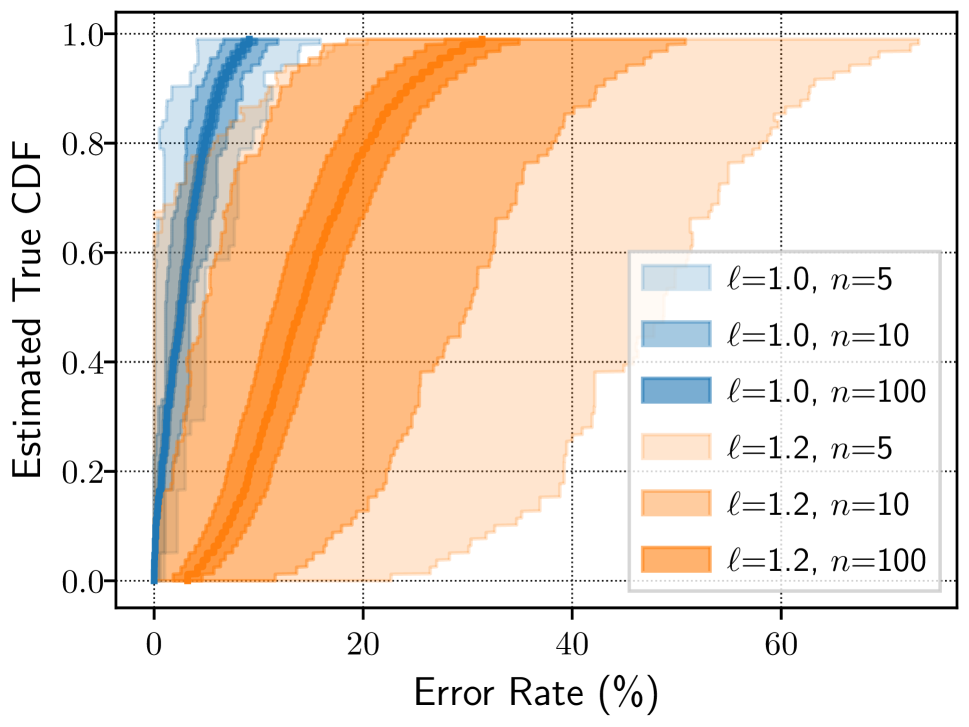
Client Download Error Rate
The client download error rate (i.e., the fraction of failed over attempted downloads) helps us understand how additional traffic load would impact usability. Larger error rates indicate a more congested network and represent a poorer user experience. We measure the number of attempted and failed downloads throughout the simulations, and compute the download error rate across all downloads (independent of file size) for each performance benchmarking client. We present in Figure 8 the download error rate across all benchmarking clients. (Note that another general network assessment metric, Tor network goodput, is shown in Figure 12 in Appendix D.)
Figure 8(a) shows the result of our statistical analysis from §5 when using a network scale of 1% (). As with the client download time metric, we see overlap in the and CIs when . Although it appears that the download error rates decrease when adding 20% load (because the range of the CI is generally to the right of the range of the CI), we are unable to draw conclusions at the desired confidence when . However, the and CIs become significantly narrower (and no longer overlap) with simulations, and it becomes clear that adding 20% load increases the error rate.
Our experiments with the network scale of 10% again offer more reliable results. Figure 8(b) shows significant overlap in the and CIs when simulations and a very slight overlap in CIs when . However, based on the estimated true CDF and CIs when , we can again confidently conclude that increasing the traffic load by 20% increases the download error rate because the CIs are clearly distinguishable. Notice that the CI precision for compared to the CI precision for offers an additional insight into the results: the error rate is more highly varied when , indicating that the user experience is much less consistent than it is when .
Finally, the results from our experiments with the network scale of 30% again reinforce our previous conclusions about our hypothesis. Figure 8(c) shows that the estimated true CDFs and their CIs are completely distinguishable, allowing us to confirm our hypothesis even when .
Conclusions
We offer some general observations based on the results of our case study. First, our results indicate that it is possible to come to similar conclusions by running experiments in networks of different scales. Generally, fewer simulations will be required to achieve a particular CI precision in networks of larger scale than in networks of smaller scale. The network scale that is appropriate and the precision that is needed will vary and depend heavily on the experiments and metrics being compared and the hypothesis being tested. However, based on our results, we suggest that networks at a scale of at least 10% () are used whenever possible, and we strongly recommend that 1% networks be avoided due to the unreliability of the results they generate. Second, some of our results exhibited the phenomenon that increasing the number of simulations also decreased the CI precision, although the opposite is expected. This behavior is due to random sampling and is more likely to be exhibited for smaller . Along with the analysis from §5, our results lead us to recommend that no fewer than simulations be run for any experiment, independent of the network scale .
7 Conclusion
In this paper, we develop foundations upon which future Tor performance research can build. The foundations we develop include: (i) a new Tor network modeling methodology and supporting tools that produce more representative Tor networks (§3); (ii) accuracy and performance improvements to the Shadow simulator that allow us to run Tor simulations faster and at a larger scale than was previously possible (§4); and (iii) a methodology for conducting statistical inference of results generated in scaled-down (sampled) Tor networks (§5). We showcase our modeling and simulation scalability improvements by running simulations with 6,489 relays and 792k users, the largest known Tor network simulations and the first at a network scale of 100% (§4.3). Building upon the above foundations, we conduct a case study of the effects of traffic load on client performance in the Tor network through a total of 420 Tor simulations across three network scale factors and two traffic load factors (§6). Our case study demonstrates how to apply our methodologies for modeling Tor networks and for conducting sound statistical inferences of results.
Conclusions
We find that: (i) significant reductions in RAM are possible by representing multiple Tor users in each Tor client process (§4.3); (ii) it is feasible to run 100% Tor network simulations on high-memory servers in a reasonable time (less than 2 weeks) (§4.3); (iii) running multiple simulations in independent Tor networks is necessary to draw statistically significant conclusions (§5); and (iv) fewer simulations are generally needed to achieve a desired CI precision in networks of larger scale than in those of smaller scale (§6).
Limitations and Future Work
Although routers in Shadow drop packets when congested (using CoDel), we describe in §3.1 that we do not model any additional artificial packet loss. However, it is possible that packet loss or corruption rates are higher in Tor than in Shadow (e.g., for mobile clients that are wirelessly connected), and modeling this loss could improve realism. Future work should consider developing a more realistic packet loss model that is, for example, based on measurements of actual Tor clients and relays.
In §3.2.1 we describe that we compute some relay characteristics (e.g., consensus weight, bandwidth rate and burst, location) using the median value of those observed across all consensus and server descriptors from the staging period. Similarly, in §3.2.2 we describe that we select relays from those available by “bucketing” them and choosing the relay with the median bandwidth capacity from each bucket. These selection criteria may not capture the full variance in the relay characteristics. Future work might consider alternative selection strategies—such as randomly sampling the full observed distribution of each characteristic, choosing based on occurrence count, or choosing uniformly at random—and evaluate how such choices affect simulation accuracy.
Our traffic modeling approach in §3.2.2 allows us to reduce the RAM required to run simulations by simulating users in each Tor client process. This optimization yields the following implications. First, we disable guards in our model because Tor does not currently support multiple guard “sessions” on a given Tor client. Future work should consider either implementing support for guard “sessions” in the Tor client, or otherwise managing guard selection and circuit assignment through the Tor control port. Second, simulating users on a Tor client results in “clustering” these users in the city that was assigned to the client, resulting in lower location diversity. Choosing values of closer to 1 would reduce this effect. Third, setting reduces the total number of Tor clients and therefore the total number of network descriptor fetches. Because these fetches occur infrequently in Tor, the network impact is negligible relative to the total amount of traffic being generated by each client.
Finally, future work might consider sampling the Tor network at scales , which could help us better understand how Tor might handle growth as it becomes more popular.
Acknowledgments
We thank our shepherd, Yixin Sun, and the anonymous reviewers for their valuable feedback. This work has been partially supported by the Office of Naval Research (ONR), the Defense Advanced Research Projects Agency (DARPA), the National Science Foundation (NSF) under award CNS-1925497, and the National Sciences and Engineering Research Council of Canada (NSERC) under award CRDPJ-534381. This research was undertaken, in part, thanks to funding from the Canada Research Chairs program. This work benefited from the use of the CrySP RIPPLE Facility at the University of Waterloo.
References
- Acquisti et al. [2003] A. Acquisti, R. Dingledine, and P. Syverson. On the Economics of Anonymity. In 7th International Financial Cryptography Conference (FC), 2003.
- AlSabah and Goldberg [2013] M. AlSabah and I. Goldberg. PCTCP: Per-circuit TCP-over-IPsec Transport for Anonymous Communication Overlay Networks. In ACM Conference on Computer and Communications Security (CCS), 2013.
- AlSabah and Goldberg [2016] M. AlSabah and I. Goldberg. Performance and Security Improvements for Tor: A Survey. ACM Computing Surveys (CSUR), 49(2):32, 2016.
- AlSabah et al. [2011] M. AlSabah, K. Bauer, I. Goldberg, D. Grunwald, D. McCoy, S. Savage, and G. M. Voelker. DefenestraTor: Throwing Out Windows in Tor. In Privacy Enhancing Technologies Symposium (PETS), pages 134–154, 2011.
- AlSabah et al. [2013] M. AlSabah, K. Bauer, T. Elahi, and I. Goldberg. The Path Less Travelled: Overcoming Tor’s Bottlenecks with Traffic Splitting. In Privacy Enhancing Technologies Symposium (PETS), 2013.
- Aryan et al. [2013] S. Aryan, H. Aryan, and J. A. Halderman. Internet Censorship in Iran: A First Look. In 3rd USENIX Workshop on Free and Open Communications on the Internet (FOCI), 2013.
- Barton and Wright [2016] A. Barton and M. Wright. DeNASA: Destination-Naive AS-Awareness in Anonymous Communications. Proceedings on Privacy Enhancing Technologies (PoPETs), 2016(4):356–372, 2016.
- Bauer et al. [2011] K. S. Bauer, M. Sherr, and D. Grunwald. ExperimenTor: A Testbed for Safe and Realistic Tor Experimentation. In USENIX Workshop on Cyber Security Experimentation and Test (CSET), 2011.
- Blumofe and Leiserson [1999] R. D. Blumofe and C. E. Leiserson. Scheduling Multithreaded Computations by Work Stealing. J. ACM, 46(5):720–748, Sept. 1999.
- Brave [2019] Brave. Brave Browser. https://brave.com/, November 2019. Accessed 2020-09-30.
- Clark et al. [2007] J. Clark, P. C. van Oorschot, and C. Adams. Usability of Anonymous Web Browsing: An Examination of Tor Interfaces and Deployability. In 3rd Symposium on Usable Privacy and Security (SOUPS), 2007.
- Conrad and Shirazi [2014] B. Conrad and F. Shirazi. Analyzing the Effectiveness of DoS Attacks on Tor. In 7th International Conference on Security of Information and Networks, page 355, 2014.
- Dahal et al. [2015] S. Dahal, J. Lee, J. Kang, and S. Shin. Analysis on End-to-End Node Selection Probability in Tor Network. In 2015 International Conference on Information Networking (ICOIN), pages 46–50, Jan 2015.
- Dingledine and Mathewson [2006] R. Dingledine and N. Mathewson. Anonymity Loves Company: Usability and the Network Effect. In 5th Workshop on the Economics of Information Security (WEIS), 2006.
- Dingledine et al. [2004] R. Dingledine, N. Mathewson, and P. Syverson. Tor: The Second-Generation Onion Router. In USENIX Security Symposium (USENIX-Sec), 2004.
- Dinh et al. [2020] T.-N. Dinh, F. Rochet, O. Pereira, and D. S. Wallach. Scaling Up Anonymous Communication with Efficient Nanopayment Channels. Proceedings on Privacy Enhancing Technologies (PoPETs), 2020(3):175–203, 2020.
- Elahi et al. [2014] T. Elahi, G. Danezis, and I. Goldberg. PrivEx: Private Collection of Traffic Statistics for Anonymous Communication Networks. In ACM Conference on Computer and Communications Security (CCS), 2014. See also git://git-crysp.uwaterloo.ca/privex.
- Fabian et al. [2010] B. Fabian, F. Goertz, S. Kunz, S. Müller, and M. Nitzsche. Privately Waiting — A Usability Analysis of the Tor Anonymity Network. In Sustainable e-Business Management, 2010.
- Fenske et al. [2017] E. Fenske, A. Mani, A. Johnson, and M. Sherr. Distributed Measurement with Private Set-Union Cardinality. In ACM Conference on Computer and Communications Security (CCS), 2017.
- Geddes et al. [2013] J. Geddes, R. Jansen, and N. Hopper. How Low Can You Go: Balancing Performance with Anonymity in Tor. In 13th Privacy Enhancing Technologies Symposium, pages 164–184, 2013.
- Geddes et al. [2014] J. Geddes, R. Jansen, and N. Hopper. IMUX: Managing Tor Connections from Two to Infinity, and Beyond. In ACM Workshop on Privacy in the Electronic Society (WPES), pages 181–190, 2014.
- Geddes et al. [2016] J. Geddes, M. Schliep, and N. Hopper. ABRA CADABRA: Magically Increasing Network Utilization in Tor by Avoiding Bottlenecks. In 15th ACM Workshop on Privacy in the Electronic Society, pages 165–176, 2016.
- Gopal and Heninger [2012] D. Gopal and N. Heninger. Torchestra: Reducing Interactive Traffic Delays over Tor. In ACM Workshop on Privacy in the Electronic Society (WPES), 2012.
- Hanley et al. [2019] H. Hanley, Y. Sun, S. Wagh, and P. Mittal. DPSelect: A Differential Privacy Based Guard Relay Selection Algorithm for Tor. Proceedings on Privacy Enhancing Technologies (PoPETs), 2019(2):166–186, 2019.
- Hoel [1971] P. G. Hoel. Introduction to Mathematical Statistics. Wiley, New York, 4th edition, 1971. ISBN 0471403652.
- Hopper [2014] N. Hopper. Challenges in protecting Tor hidden services from botnet abuse. In Financial Cryptography and Data Security (FC), pages 316–325, 2014.
- Imani et al. [2018] M. Imani, A. Barton, and M. Wright. Guard Sets in Tor using AS Relationships. Proceedings on Privacy Enhancing Technologies (PoPETs), 2018(1):145–165, 2018.
- Imani et al. [2019] M. Imani, M. Amirabadi, and M. Wright. Modified Relay Selection and Circuit Selection for Faster Tor. IET Communications, 13(17):2723–2734, 2019.
- Jansen and Hopper [2012] R. Jansen and N. Hopper. Shadow: Running Tor in a Box for Accurate and Efficient Experimentation. In Network and Distributed System Security Symposium (NDSS), 2012. See also https://shadow.github.io.
- Jansen and Johnson [2016] R. Jansen and A. Johnson. Safely Measuring Tor. In ACM Conference on Computer and Communications Security (CCS), 2016. See also https://github.com/privcount.
- Jansen et al. [2010] R. Jansen, N. Hopper, and Y. Kim. Recruiting New Tor Relays with BRAIDS. In ACM Conference on Computer and Communications Security (CCS), 2010.
- Jansen et al. [2012a] R. Jansen, K. Bauer, N. Hopper, and R. Dingledine. Methodically Modeling the Tor Network. In USENIX Workshop on Cyber Security Experimentation and Test (CSET), 2012a.
- Jansen et al. [2012b] R. Jansen, P. F. Syverson, and N. Hopper. Throttling Tor Bandwidth Parasites. In USENIX Security Symposium (USENIX-Sec), 2012b.
- Jansen et al. [2013] R. Jansen, A. Johnson, and P. Syverson. LIRA: Lightweight Incentivized Routing for Anonymity. In Network and Distributed System Security Symposium (NDSS), 2013.
- Jansen et al. [2014a] R. Jansen, J. Geddes, C. Wacek, M. Sherr, and P. Syverson. Never Been KIST: Tor’s Congestion Management Blossoms with Kernel-Informed Socket Transport. In USENIX Security Symposium (USENIX-Sec), 2014a.
- Jansen et al. [2014b] R. Jansen, F. Tschorsch, A. Johnson, and B. Scheuermann. The Sniper Attack: Anonymously Deanonymizing and Disabling the Tor Network. In Network and Distributed System Security Symposium (NDSS), 2014b.
- Jansen et al. [2018a] R. Jansen, M. Traudt, J. Geddes, C. Wacek, M. Sherr, and P. Syverson. KIST: Kernel-Informed Socket Transport for Tor. ACM Transactions on Privacy and Security (TOPS), 22(1):3:1–3:37, December 2018a.
- Jansen et al. [2018b] R. Jansen, M. Traudt, and N. Hopper. Privacy-Preserving Dynamic Learning of Tor Network Traffic. In ACM Conference on Computer and Communications Security (CCS), 2018b. See also https://tmodel-ccs2018.github.io.
- Jansen et al. [2019] R. Jansen, T. Vaidya, and M. Sherr. Point Break: A Study of Bandwidth Denial-of-Service Attacks against Tor. In USENIX Security Symposium (USENIX-Sec), 2019.
- Johnson et al. [2017a] A. Johnson, R. Jansen, N. Hopper, A. Segal, and P. Syverson. PeerFlow: Secure Load Balancing in Tor. Proceedings on Privacy Enhancing Technologies (PoPETs), 2017(2):74–94, 2017a.
- Johnson et al. [2017b] A. Johnson, R. Jansen, A. D. Jaggard, J. Feigenbaum, and P. Syverson. Avoiding The Man on the Wire: Improving Tor’s Security with Trust-Aware Path Selection. In Network and Distributed System Security Symposium (NDSS), 2017b.
- Kiran et al. [2019] K. Kiran, S. S. Chalke, M. Usman, P. D. Shenoy, and K. Venugopal. Anonymity and Performance Analysis of Stream Isolation in Tor Network. In International Conference on Computing, Communication and Networking Technologies (ICCCNT), 2019.
- Komlo et al. [2020] C. H. Komlo, N. Mathewson, and I. Goldberg. Walking onions: Scaling anonymity networks while protecting users. In USENIX Security Symposium (USENIX-Sec), 2020.
- Lakshmikantha et al. [2008] A. Lakshmikantha, R. Srikant, and C. Beck. Impact of File Arrivals and Departures on Buffer Sizing in Core Routers. In IEEE INFOCOM 2008 - The 27th Conference on Computer Communications, May 2008.
- Lee et al. [2017] L. Lee, D. Fifield, N. Malkin, G. Iyer, S. Egelman, and D. Wagner. A Usability Evaluation of Tor Launcher. Proceedings on Privacy Enhancing Technologies (PoPETs), 2017, 07 2017.
- Lin et al. [2016] D. Lin, M. Sherr, and B. T. Loo. Scalable and Anonymous Group Communication with MTor. Proceedings on Privacy Enhancing Technologies (PoPETs), 2016(2):22–39, 2016.
- Liu et al. [2017] Z. Liu, Y. Liu, P. Winter, P. Mittal, and Y.-C. Hu. TorPolice: Towards Enforcing Service-Defined Access Policies for Anonymous Communication in the Tor Network. In International Conference on Network Protocols, 2017.
- Loesing et al. [2010] K. Loesing, S. J. Murdoch, and R. Dingledine. A Case Study on Measuring Statistical Data in the Tor Anonymity Network. In Financial Cryptography and Data Security (FC), 2010. See also https://metrics.torproject.org.
- Mani and Sherr [2017] A. Mani and M. Sherr. HisTor: Differentially Private and Robust Statistics Collection for Tor. In Network and Distributed System Security Symposium (NDSS), 2017.
- Mani et al. [2018] A. Mani, T. Wilson-Brown, R. Jansen, A. Johnson, and M. Sherr. Understanding Tor Usage with Privacy-Preserving Measurement. In 18th ACM Internet Measurement Conference (IMC), 2018. See also https://torusage-imc2018.github.io.
- Miller and Jansen [2015] A. Miller and R. Jansen. Shadow-Bitcoin: Scalable Simulation via Direct Execution of Multi-threaded Applications. In USENIX Workshop on Cyber Security Experimentation and Test (CSET), 2015.
- Mitseva et al. [2020] A. Mitseva, M. Aleksandrova, T. Engel, and A. Panchenko. Security and Performance Implications of BGP Rerouting-Resistant Guard Selection Algorithms for Tor. In IFIP International Conference on ICT Systems Security and Privacy Protection, 2020.
- Moore et al. [2011] W. B. Moore, C. Wacek, and M. Sherr. Exploring the Potential Benefits of Expanded Rate Limiting in Tor: Slow and Steady Wins the Race with Tortoise. In Annual Computer Security Applications Conference (ACSAC), 2011.
- Mozilla [2019] Mozilla. Mozilla Research Grants 2019H1. https://mozilla-research.forms.fm/mozilla-research-grants-2019h1/forms/6510, 2019. Call for Proposals.
- Mozilla [2019] Mozilla. Firefox Public Data Report. https://data.firefox.com/dashboard/user-activity, December 2019.
- Ngan et al. [2010] T.-W. J. Ngan, R. Dingledine, and D. S. Wallach. Building Incentives into Tor. In Financial Cryptography and Data Security (FC), 2010.
- Norcie et al. [2012] G. Norcie, K. Caine, and L. J. Camp. Eliminating Stop-Points in the Installation and Use of Anonymity Systems: a Usability Evaluation of the Tor Browser Bundle. In Privacy Enhancing Technologies Symposium (PETS), 2012.
- Rochet and Pereira [2017] F. Rochet and O. Pereira. Waterfilling: Balancing the Tor network with maximum diversity. Proceedings on Privacy Enhancing Technologies (PoPETs), 2017(2):4–22, 2017.
- Rochet and Pereira [2018] F. Rochet and O. Pereira. Dropping on the Edge: Flexibility and Traffic Confirmation in Onion Routing Protocols. Proceedings on Privacy Enhancing Technologies (PoPETs), 2018(2):27–46, 2018.
- Rochet et al. [2020] F. Rochet, R. Wails, A. Johnson, P. Mittal, and O. Pereira. CLAPS: Client-Location-Aware Path Selection in Tor. In ACM Conference on Computer and Communications Security (CCS), 2020.
- Shirazi et al. [2015a] F. Shirazi, C. Diaz, and J. Wright. Towards Measuring Resilience in Anonymous Communication Networks. In 14th ACM Workshop on Privacy in the Electronic Society, pages 95–99, 2015a.
- Shirazi et al. [2015b] F. Shirazi, M. Goehring, and C. Diaz. Tor Experimentation Tools. In International Workshop on Privacy Engineering (IWPE), 2015b.
- Singh [2014] S. Singh. Large-Scale Emulation of Anonymous Communication Networks. Master’s thesis, University of Waterloo, 2014.
- Tang and Goldberg [2010] C. Tang and I. Goldberg. An Improved Algorithm for Tor Circuit Scheduling. In 17th ACM Conference on Computer and Communications Security (CCS), 2010.
- [65] The Tor Project. Mozilla Research Call: Tune up Tor for Integration and Scale. https://blog.torproject.org/mozilla-research-call-tune-tor-integration-and-scale, May 2019. Blog Post.
- The Tor Project [2020a] The Tor Project. Tor Metrics Portal. https://metrics.torproject.org, January 2020a.
- The Tor Project [2020b] The Tor Project. Reproducible Metrics. https://metrics.torproject.org/reproducible-metrics.html#performance, October 2020b.
- The Tor Project [2020c] The Tor Project. The Tor Project. https://www.torproject.org, January 2020c.
- Tracey et al. [2018] J. Tracey, R. Jansen, and I. Goldberg. High Performance Tor Experimentation from the Magic of Dynamic ELFs. In USENIX Workshop on Cyber Security Experimentation and Test (CSET), 2018.
- Unger [2018] N. Unger. NetMirage. https://crysp.uwaterloo.ca/software/netmirage/, 2018. Accessed 2020-02-12.
- United Nations [2020] United Nations. Freedom of Information. https://www.un.org/ruleoflaw/thematic-areas/governance/freedom-of-information, January 2020.
- Vahdat et al. [2003] A. Vahdat, K. Yocum, K. Walsh, P. Mahadevan, D. Kostić, J. Chase, and D. Becker. Scalability and Accuracy in a Large-Scale Network Emulator. SIGOPS Oper. Syst. Rev., 36(SI):271–284, Dec. 2003.
- Wacek et al. [2013] C. Wacek, H. Tan, K. Bauer, and M. Sherr. An Empirical Evaluation of Relay Selection in Tor. In Network and Distributed System Security Symposium (NDSS), 2013.
- Yang and Li [2015a] L. Yang and F. Li. mTor: A Multipath Tor Routing Beyond Bandwidth Throttling. In 2015 IEEE Conference on Communications and Network Security (CNS), pages 479–487, Sept 2015a.
- Yang and Li [2015b] L. Yang and F. Li. Enhancing Traffic Analysis Resistance for Tor Hidden Services with Multipath Routing. In International Conference on Security and Privacy in Communication Systems, pages 367–384, 2015b.
Appendix
Appendix A Ontology of Tor Performance Metrics
|
latency |
jitter |
bandwidth |
reliability |
packet loss |
path/routing |
congestion |
time to Tor consensus |
time to steady state
|
quantity |
IP address |
geolocation |
stack |
OS/kernel |
hardware |
CPU/memory usage |
throughput |
goodput |
control overhead |
retransmissions
|
behavior model |
number of connections |
duration of connections |
traffic type |
idle time |
time to first/last byte |
Tor |
relay selection algorithm |
max num. open circuits |
max duration of circuits |
circuit build time |
errors
|
Tor relay configuration |
packet delay |
congestion |
processing (Tor) |
processing (stack) |
connections (number of:) |
sockets open |
streams and circuits |
connecting clients |
errors
|
behavior model |
port |
|
| Indep. | - | - | - | - | - | - | - | - | - | - | - | - | - | - | - | - | - | - | - | |||||||||||||||||||||||||
| Dep. | - | - | - | - | - | - | - | - | - | - | - | - | - | - | - | - | - | - | ||||||||||||||||||||||||||
| Network | Common | Clients | Relays | Servers | ||||||||||||||||||||||||||||||||||||||||
| Network Nodes | ||||||||||||||||||||||||||||||||||||||||||||
| Property | Description | ||
| Network | latency | The amount of time it takes for a packet to traverse from one network node to another. | |
| jitter | The variation in latency. | ||
| bandwidth | The amount of data a network connection can transfer in a given amount of time. | ||
| reliability | The probability of a network connection successfully transferring data. | ||
| packet loss | The probability of a packet on an existing connection not arriving at the destination. | ||
| path/routing | The set of network nodes a packet passes through to arrive at its destination. | ||
| congestion | The amount of traffic load exceeding the capacity of the link or network node. | ||
| time to Tor consensus | The amount of time until the Tor network generates a valid consensus file (the file directory authorities publish containing information about every relay). | ||
| time to steady state | The amount of time until the network displays consistent behavior. | ||
| Network Nodes | Common | quantity | The amount of this particular type of node in the network. |
| IP address | The external IP address of the node. | ||
| geolocation | Where the node is geographically located. | ||
| stack | What Tor and associated processes are running on. | ||
| OS/kernel | The operating system, especially the network stack. | ||
| hardware | The computer components and their characteristics, such as CPU speed and memory capacity. | ||
| CPU/memory usage | The amount of CPU time and RAM used. | ||
| throughput | The total network traffic seen in a given amount of time, including overhead such as packet headers and retransmissions. | ||
| goodput | The total amount of usable traffic seen in a given amount of time, therefore not including overhead from headers or retransmissions. | ||
| control overhead | The amount of traffic that is spent on protocol data, rather than payload data. | ||
| retransmissions | The amount of traffic that was duplicated as a result of TCP acknowledgements not being received (in time). | ||
| Clients | behavior model | How the client behaves. | |
| number of connections | How many network connections the client creates (typically to servers, via Tor relays). | ||
| duration of connections | How long network connections last before being closed. | ||
| traffic type | The protocol and traffic properties (e.g., web pages, large downloads). | ||
| idle time | The time spent not sending any traffic, either because there is nothing being sent over a currently active connection, or because the client has completed all connections and has not yet started another. | ||
| time to first byte | The amount of time it takes to receive the first byte of a download. Also known as round trip time (RTT). | ||
| time to last byte | The amount of time it takes to complete a download. | ||
| Tor | |||
| relay selection algorithm | How Tor chooses which relays to route through. | ||
| max number of open circuits | The maximum number of Tor circuits simultaneously open. | ||
| max duration of circuits | The maximum amount of time circuits remain open. | ||
| circuit build time | How long it takes to construct a circuit. | ||
| errors | The number and characteristics of errors encountered. | ||
| Relays | Tor relay configuration | The configuration of the Tor relay, whether in configuration files or changes to the Tor application. | |
| packet delay | The amount of additional time it takes for a packet to enter and leave the entire relay. | ||
| congestion | Network congestion specifically as a result of the Tor relay process. | ||
| processing (Tor) | The amount of time spent processing packets within the Tor process. | ||
| processing (stack) | The amount of time spent processing packets outside the Tor process (primarily the OS). | ||
| connections (number of:) | |||
| sockets open | The number of network sockets the relay has open. | ||
| streams and circuits | The number of TCP streams and Tor circuits. | ||
| connecting clients | The number of clients that connect to this relay. | ||
| errors | The number and characteristics of errors encountered. | ||
| Servers | behavior model | How the server interacts with the client application communicating with it. | |
| port | The network ports the server is listening on. This is distinct from the behavior model in that Tor relays interact with it (via exit policies), not just the client. | ||
In this appendix, we describe an ontology of the Tor network, from the perspective and for the purpose of controlled performance research. While our ontology shows one way of orienting known factors to consider when conducting Tor experiments, we emphasize that it is not intended to be complete. The most interesting future research may come not from the measurement of properties (or even elements) listed here, but from the gaps and undervalued areas that are currently unexplored in Tor research.
Ontology
The ontology consists of elements (clients, relays, servers, and the network), each of which have properties that can be further recursively subdivided into (sub)properties. These properties can be viewed as the variables of an experiment, and therefore can be separated into independent and dependent variables. Independent variables are properties that are set, chosen during the course of experiment configuration (e.g., the number of clients, or available bandwidth). Dependent variables are properties that can be measured as results of the experiment (e.g., throughput, or successful downloads). The division between what constitutes independent and dependent variables depends on the specific context of an experiment. In this ontology, we classified properties based on the experimentation platforms we examined. Specifically, these categorizations are based on controlled Tor experiments; more observational research (e.g., the measurements done on Tor Metrics [66]) would have a different perspective, primarily manifesting as many properties shifting from independent to dependent variables. Even with this particular point of reference, however, some properties can concurrently exist as both independent and dependent variables in one experiment. Packet loss, for example, is something that can be configured as a property of the network (i.e., a particular link can be configured to drop packets with some probability), but will also occur as a result of the natural behavior of TCP stacks establishing a stable connection and can therefore be measured.
Network
The network element represents the connections between other elements, as well as meta-properties that are not directly measurable on individual nodes (though analogues may be). Latency and bandwidth, for example, are properties directly instantiated in the links between the other elements. The time to a steady state, on the other hand, is something that can be measured, but not as an actual property of any particular element, so much as a measurement of a constructed representation of the network itself.
Network Nodes
Network nodes are all endpoints in the network (i.e., every client, relay, and server). While we could assign their common properties to each of the elements discussed in the remainder of this section, we group them together to reflect their commonality (and to conserve space).
Some properties, such as control overhead, could arguably be positioned as part of the network itself, but are in this ontology considered part of the network nodes. The deciding factor was whether the variable could be directly configured or measured as a property of a particular node. For example, while packet loss requires knowledge of the link between two relays, control overhead can be measured on only one end; therefore, we place the former as a network property and the latter as a property of the network node. From a more empirical perspective, tools such as Shadow and NetMirage would configure/measure packet loss on the edges of a network graph, while control overhead would be measured using data collected from the node.
Clients
Clients are the subclass of network nodes that run applications proxied via Tor; they represent both normal Tor clients, as well as onion services. Client properties include those relating to the Tor application itself, as well as the application(s) being proxied through it.
Relays
Relays are the subclass of network nodes that run Tor relays. As above, relay properties include those of the Tor application, as well as the environment in which it runs.
Servers
Servers are the subclass of network nodes that represent non-Tor network entities; e.g., web servers and non-Tor clients. Because they do not run Tor, and will typically be creating requests or responding to requests created elsewhere, they add few properties not already captured above.
Appendix B Description of Tor Modeling Tools
Here we provide additional details about the Tor modeling tools that we described in §3.2.3.
TorNetTools
We wrote a new Tor modeling tool called TorNetTools as a Python package (3,034 LoC) to make our work more accessible. The tool guides researchers through the experimentation process, including staging and generating network models, simulating the models, and analyzing and visualizing the results. The tool implements our modeling algorithms from §3.2.2, producing valid configuration files that can immediately be used to run Tor experiments in our Tor experimentation platform as we describe in §4. The tool also implements our statistical analysis methodology from §5, including the computation and visualization of confidence intervals when plotting CDFs. TorNetTools v1.1.0 was released in conjunction with this work.151515https://github.com/shadow/tornettools
TGen
We significantly extended and enhanced the TGen traffic generator [38, §5.1] (6,531 LoC added/modified and 1,411 removed) to support our traffic generation models. Our improvements include refactoring and generalizing the generator component so that it can continuously generate flows in addition to streams and packets. We also refactored and extended the stream component to support deterministic execution of the models, which allows the client and server sides to synchronize the traffic generation process by exchanging a seed rather than exchanging the full models during each stream handshake. Finally, we extended encoding and validation of Markov models and added support for the normal, Pareto, and uniform probability distributions (in addition to the already-supported log-normal and exponential distributions) to support further exploration of new traffic models. TGen v1.0.0 was released in conjunction with this work.161616https://github.com/shadow/tgen
OnionTrace
We implemented a new tool called OnionTrace (2,594 LoC) to interact with a Tor process during an experiment. OnionTrace supports three modes. In log mode, it connects to Tor over Tor’s control port, registers for various asynchronous events (e.g., bytes sent and received every second), and logs this information to a file for later analysis. In record mode, it extracts information about the circuits and streams that a Tor process creates over time and stores it in a CSV file. In playback mode, it reads a previously recorded CSV file and forces Tor to build the same set of circuits at the same time as indicated in the file. By using record and playback mode in successive experiments, a researcher can be sure that the same set of circuits with the same chosen relays are used across both experiments, improving reproducibility. OnionTrace v1.0.0 was released in conjunction with this work.171717https://github.com/shadow/oniontrace
Appendix C Description of Shadow Improvements
Here we provide additional details about the improvements we made to the Shadow simulator that we introduced in §4.2. Our improvements have been merged into Shadow v1.13.2.181818https://github.com/shadow/shadow
Determinism
We corrected some bugs in Shadow that caused it to produce non-deterministic behavior in host IP address assignment and the processing order of packet events.
Run-time Optimizations
Through analysis with the performance analysis tool perf, we identified a bottleneck in Shadow’s epoll I/O event notification facility; our fix reduced run time by 40% in a small Tor test network.
Bootstrapping
We added a new feature that allows configuration of a startup phase where Shadow will not enforce bandwidth limits or drop packets, reducing Tor bootstrapping time from 20 to 5 simulated minutes.
Connection Limit
We associated network connections by <src_ip, src_port, dst_ip, dst_port, protocol>, allowing each host to support connections to every other host rather than connections globally.
Network Stack
We implemented delayed acknowledgments (to reduce the number of empty ACKs), and explicit duplicate ACKs (to correctly trigger “3 duplicate ACK” TCP events). We updated the TCP auto-tuning algorithm so that it uses the RTT of the peers. Finally, we corrected a bug by setting packet retransmission timers and header timestamps when packets are sent rather than when they are queued to be sent.
Appendix D Additional Performance Results
We supplement the analysis done in §6.3 with additional plots of performance metrics measured across our 420 simulations following our statistical inference methodology from §5. Our supplemental results include the transfer times measured by the performance benchmarking clients: the time to first byte across all transfer sizes are shown in Figure 9, while the time to last byte of 50 KiB and 5 MiB transfers are shown in Figures 10 and 11, respectively. The total Tor network goodput (summed over all relays) is shown in Figure 12.


