On weight and variance uncertainty in neural networks for regression tasks
Abstract
We consider the problem of weight uncertainty proposed by [Blundell et al. (2015). Weight uncertainty in neural network. In International conference on machine learning, 1613-1622, PMLR.] in neural networks (NNs) specialized for regression tasks. We further investigate the effect of variance uncertainty in their model. We show that including the variance uncertainty can improve the prediction performance of the Bayesian NN. Variance uncertainty enhances the generalization of the model by considering the posterior distribution over the variance parameter. We examine the generalization ability of the proposed model using a function approximation example and further illustrate it with the riboflavin genetic data set. We explore fully connected dense networks and dropout NNs with Gaussian and spike-and-slab priors, respectively, for the network weights.
Keywords: Bayesian neural networks, Variational Bayes, Kullback-Leibler divergence, posterior distribution, Regression task, variance uncertainty.
1 Introduction
Bayesian Neural Networks (BNNs) have been introduced and comprehensively discussed by many authors (among others see [14, 2]). BNNs are suitable for modeling uncertainty by considering values of the parameters that might not be learned by the available data. This is achieved by randomizing unknown parameters, such as weights and biases while incorporating prior knowledge. Such an approach naturally regularizes the model and helps prevent overfitting, a common challenge in neural networks (NNs). The BNNs can also be considered as a suitable and more reliable alternative to ensemble learning methods [15], including bagging and boosting of the neural networks.
The primary objective in the BNNs is to estimate the posterior distribution of the parameters. However, obtaining the exact posterior is often infeasible due to the integrals’ intractability. Thus, it is necessary to use approximation techniques for the posterior density. One common approach is the Markov Chain Monte Carlo (MCMC), including the Metropolis-Hastings algorithm [10], which generates samples from the posterior distribution by constructing a Markov chain, typically of first orders.
Despite its effectiveness, flexibility, and strong theoretical foundations, MCMC has significant limitations in high-dimensional spaces, including slow convergence and high computational costs. Variational Bayes (VB) has emerged as a faster and more scalable approximation technique. First introduced by [11] and [19], VB seeks to approximate the intractable posterior distribution by identifying a simpler, parametric probability distribution that closely resembles the true posterior. The central idea in VB is to recast the problem of posterior inference as an optimization task. Specifically, VB minimizes the Kullback-Leibler (KL) divergence [13] between the approximate distribution and the true posterior [3]. This involves iteratively updating the hyper-parameters of the approximate distribution to improve its fit to the posterior while maintaining computational efficiency [1].
The VB method has limitations related to the conjugacy of the full conditionals of parameters. In such cases, models that go beyond the conjugacy of the exponential family have been proposed [20]. Black Box Variational Inference (BBVI) [16] eliminates the need for conditional conjugacy by introducing a flexible framework for approximating posterior distributions. It leverages stochastic optimization techniques to estimate gradients and employs variance reduction strategies to enhance computational efficiency and stability. Bayes by Backprop (weight uncertainty), introduced by Blundell et al. [4], is another approach for performing Bayesian inference in NNs. This method leverages stochastic optimization and employs the re-parametrization trick to enable efficient sampling and gradient-based optimization of posterior distributions, for a NN weights. The model is used for classification and regression tasks, by considering suitable multi-nomial and Gaussian likelihood for the target variable, respectively.
Another approach for modeling uncertainty in weights of a NN is considered in [7]. They modeled the variational approximation of the weights as the multiplication of a fixed hyperparameter (which might be optimized) by a bernoulli random varaible for modeling the droupout mechanism. There are two main differences between the method considered in [7] and that in [4]. The first difference is that no statistical distribution is considered for modelling uncertainty in weights around the hyperparameter in the method proposed in [7]. The second difference is the approach for modeling the dropout mechanishm, since the dropout mechinism was modeled by considering the slab-and-spike prior for the weights of the NN in [4].
For the regression task, the variance of the Gaussian likelihood is assumed fixed in [4] and is determined by cross-validation. In this paper, we consider the problem of variance uncertainty in the model proposed by [4] to investigate its effectiveness on the prediction performance of the BNNs for regression tasks. Throughout a simulation study from a nonlinear function approximation problem, it is shown that the Bayes by Backprop with variance uncertainty performs better than the model with fixed variance. We have also considered the riboflavin data set, which is a genetic high dimensional data set to evaluate the performance of the proposed model, compared to the other methods, by applying PCA-BNN and the dropout-BNN methods. The dropout-BNN is applied by considering the spike-and-slab prior for the weights of the BNN. As the results presented in Section 6 shows, our proposed method outperforms other approaches in terms of MSPE and coverage probabilities for the regression curve, as well as MSPE for the riboflavin dataset.
The remainder of the paper is organized as follows. Section 2 reviews the foundations of the BNNs. The VB method for posterior approximation is introduced in Section 3. Section 4 describes the Bayes by Backprop method proposed by [4], for the regression task with fixed variance. In Section 5, we propose the variance uncertainty for the BNNs. The experimental results and the evaluation of the proposed model is considered in Section 6. Some concluding remarks are given in Section 7. The codes for this study is available online on github (soon).
2 Bayesian Neural Networks
In this section, our goal is to describe BNNs and their challenges in practical applications. Before examining BNNs, we briefly describe NNs from a statistical perspective. A NN aims to approximate the unknown function where and are the input and the output vectors, respectively. From a statistical point of view, given the sample points , the objective function of NN is the log-likelihood function of weights and biases, , and extra parameters , of the model, which is aimed to be maximized to learn the parameters of the network
The likelihood function depends on the specific problem being addressed:
-
•
In regression tasks, the likelihood function is typically modeled by a Gaussian density of with a mean provided by the network given the input data set and an unknown variance , and the negative log-likelihood corresponds to the sum of squared errors (SSE).
-
•
In classification problems, the likelihood function is often modeled as a categorical distribution, and the negative log-likelihood corresponds to the cross-entropy loss.
In a BNN, a prior distribution is considered for the parameters of the model [14], and our goal is to find a posterior distribution of all parameters . Using the Bayes’ formula, the posterior density is obtained as
where is the marginal distribution of the data, given by
The point estimation of the model parameters might be computed by the maximum a posteriori (MAP) estimator as follows
The posterior predictive distribution function, used to make predictions and to determine prediction intervals for new data, is defined as follows (for more details, see e.g., [14, 2])
In practice, we face intractable integrals to solve ; therefore, we resort to approximation methods. In the following, we introduce VB as a well-known approximation technique.
3 Variational Bayes
The VB is a method for finding an approximate distribution of the posterior distribution , by minimizing the Kullback-Leibler divergence as a measure of closeness [18]. In this section, we briefly review the basic elements of the VB method.
Let be a vector of observed data, and be a parameter vector with joint distribution . In the Bayesian inference framework, the inference about is done based on the posterior distribution where .
In the VB method, we assume the parameter vector is divided into partitions and we want to approximate by
where is the variational posterior over the vector of posterior parameters . Hence, each can be a vector of parameters. The best VB approximation is then obtained as
where
| (1) |
Let be the partitions of hyper-parameter such that each be the variational parameter of . In the fixed-form-VB (FFVB), we consider an assumed density function for each , with unknown , and we aim to determine the hyper-parameters such that is minimized.
It is clear from (1) that minimizing KL is equivalent to maximizing the evidence lower bound (ELBO) with respect to , defined as
The ELBO is equal to when the KL divergence is zero, meaning a perfect fit. The closer the value of to (greater values), the fit is better. Maximizing the ELBO is equivalent to minimizing its negative. It follows that
where represents the optimal parameter estimate for maximizing the ELBO.
We define a loss function to be minimized. Assume that is a random variable with a probability density function , and let be a function. In this case, as shown in [4], if
| (2) |
then
| (3) |
Equation (3) shows that if we can find a transformation for such that it depends on and satisfies the condition (2), then samples of can be used to generate samples of . This approach focuses on finding , as defined above. Therefore, we define
| (4) |
Note that the expectation of is the negative of the ELBO and the gradient of provides an unbiased estimate of the gradient defined in equation (3). In addition, increasing the number of samples of reduces the variance of the estimated gradient. This method utilizes equation (4) as an objective function to determine .
4 Variational Bayes Regression Network with Fixed Variance
In this section, we consider regression problems with constant variance. As we mentioned in section 3, we can use equation (4) for the optimization problem as the KL error and we are interested in minimizing it.
Following the approach described in [4], the variance of the likelihood function in a regression problem can be fixed to a constant value. In regression problems, assuming independency among the output features (i.e., the values of the vector ), we have
where is the identity matrix, represents the -th input variable, denotes the -th output variable, , and is a fixed known variance. Moreover, represents the output of a NN with an arbitrary number of layers. In this case, we have the conditional distribution
If is the th observation, then the likelihood function, assuming independent observations, is given by
Thus, [4] considered the objective function
| (5) |
with
and , seeking the optimum value of . We denote this method by VBNET-FIXED throughout the remaining of the paper. However, this approach fails to effectively capture uncertainty in the variance parameter. In the forthcoming section, we will discuss how to introduce uncertainty in the variance by using parametrization, so that the model can be generalized by considering the posterior distribution over the variance parameter.
5 Variational Bayes Regression Network with Variance Uncertainty
In this section, we suggest to use a variational posterior distribution over weights, biases, and also the variance of the likelihood function. Our proposal can be considered as a generalization of the previous model introduced in section 4. In our approach, we assume that the posterior parameters are represented by , where encompasses the weights and biases of the NN, and denotes a parameter related to the variance of the likelihood function. Additionally, we define the variational parameters as , where and pertain to the variational distribution over , and and are associated to variational distribution over .
Recall in a regression task we have
that gives
Therefore, the likelihood function has form
Based on [4], we assume that the variational posterior of all parameters is a diagonal Gaussian distribution, i.e., , where denotes the number of weights and biases in the NN, and . Also let
such that
Further, assume and . Then, the posterior samples of and are given by
where denotes element-wise multiplication. Here, and are the variational parameters associated with , and and are the variational parameters associated with .
Algorithm 1 describes the VB algorithm for the regression network with variance uncertainty. We denote this method by VBNET-SVAR throughout the remaining of the paper.
6 Experimental Results
In this section, we evaluate the results of our proposed model on two regression problems under the following scenarios
-
•
The normal prior, which corresponds to a normal distribution, assuming independency between the prior over parameters, is given by
where denotes the variance of the prior, and represents the vector of parameters.
-
•
The spike-and-slab prior [8], which corresponds to a mixture of normal distributions, assuming independency between the prior over parameters, is given by
where, represents the th (weight or bias) parameter in the model, denotes the variance of the first mixture component, which is greater than , the variance of the second mixture component, and
The second variance is assumed to be small (), allowing the prior to concentrate samples around 0 with probability .
We compare the performance of our proposed model with various models, including the model introduced in [4], and the frequentist NN. The results indicate that variance uncertainty can significantly enhance performance. It should be noted that in the nonlinear function estimation study, we have set the fixed variance for the model proposed by [4] to the train set MSE of the frequentist NN, while in the riboflavin data analysis, the fixed variance is set to the maximum of and the train set MSE of the frequentist NN to prevent the overfit small error problem caused by the frequentist NN. These values are chosen by trial and error to obtain the best performance of the model of [4] (instead of a cross-validation approach).
6.1 Nonlinear function estimation
Assume that in the problem of regression curve, the target variable is generated according to the model of the following curve.
where . To model the out-of-sample unforeseen risks, the values of for the train and test samples are generated from uniform distributions with supports and , respectively. The train and test sets contain 800 and 200 samples, respectively.


The prior is used for the VBNET-FIXED, while and the prior is considered for the VBNET-SVAR. Four competitive models are considered for the comparison study; VBNET-SVAR, VBNET-FIXED, the standard NN (NNET), and the Generalized Additive Model (GAM [9]). A total number of 10 replications is performed in this simulation study.
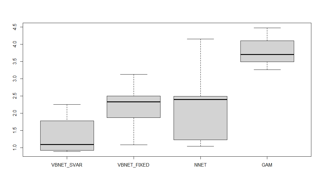
Figure 1 shows the estimated curves for all competitive models, in which the two Bayesian models also include 95% prediction intervals. Figure 2 presents box plots for the values of the Mean Squared Prediction Error (MSPE) for each model, defined as follows
where are the target values of the test set, and is the predicted value for . From Figure 2, one can observe that the VBNET-SVAR model performs better than the other competitive models for out-of-sample prediction. Figure 3 shows the box plot for the coverage probabilities of the two Bayesian models for the test set, demonstrating that the VBNET-SVAR model provides more data coverage for the out-of-sample prediction purpose.
6.2 Riboflavin dataset
Riboflavin is a dataset with a small number of samples but many features. This makes it a suitable dataset for Bayesian models. Dataset of riboflavin production by Bacillus subtilis [5] contains n = 71 observations of p = 4088 predictors (gene expressions) and a one-dimensional response (riboflavin production). From 71 samples, 56 randomly drawn samples are considered as the train set, and the remaining 25 samples are considered as the test set. We have repeated this sampling 10 times to evaluate the performance of the competitor models on this data set. All network was constructed using two hidden layers with 128 and 64 neurons, respectively.
Two scenarios are examined for fitting the NN on the train set. In the first scenario (PCA-BNN), the first 25 principal components of the 4088 genes are considered as the input of the neural network and all other competitive models. The second scenario (dropout-BNN) utilizes the feature selection using the dropout mechanism, imposed on the BNNs by the spike-and-slab prior. For the second scenario, the GAM model is replaced by the sparse-GAM model (GAMSEL) [6].


Figures 4 and 6 shows the predicted values for all competitive models, for the PCA-BNN and dropout-BNN scenarios, respectively, including 95% prediction intervals for the BNNs. Figures 5 and 7 presents box plots for the values of the MSPE for each model,for the PCA-BNN and dropout-BNN scenarios, respectively. From Figures 5 and 7, one can observe that the VBNET-SVAR model outperforms the other competitive models for out-of-sample prediction.
7 Concluding remarks
In this paper, we considered variance uncertainty in neural networks, specialized for the regression tasks. Based on the MSPE and coverage probabilities, a simulation study of a simple function approximation problem and a real genetic data set analysis showed that the prediction performance of the BNN improved by considering variance uncertainty. This method applies when no information is available regarding the variance setting of the likelihood function, which is common in many real-world applications. This model can also generalize BNNs in regression problems with fixed variance. The code for this study is available online at github (https://github.com/mortamini/vbnet).
References
- [1] Ahmed, A., Aly, M., Gonzalez, J., Narayanamurthy, S., & Smola, A. J. (2012, February). Scalable inference in latent variable models. In Proceedings of the fifth ACM International Conference on Web Search and Data Mining (pp. 123-132).
- [2] Bishop, C. M. (1997). Bayesian neural networks. Journal of the Brazilian Computer Society, 4, 61-68.
- [3] Blei, D. M., Kucukelbir, A., & McAuliffe, J. D. (2017). Variational inference: A review for statisticians. Journal of the American Statistical Association, 112(518), 859-877.
- [4] Blundell, C., Cornebise, J., Kavukcuoglu, K., & Wierstra, D. (2015, June). Weight uncertainty in neural network. In International Conference on Machine Learning (pp. 1613-1622). PMLR.
- [5] Bühlmann, P., Kalisch, M., & Meier, L. (2014). High-dimensional statistics with a view toward applications in biology. Annual Review of Statistics and Its Application, 1(1), 255-278.
- [6] Chouldechova, A., & Hastie, T. (2015). Generalized additive model selection. arXiv preprint arXiv:1506.03850.
- [7] Gal, Y., & Ghahramani, Z. (2016, June). Dropout as a bayesian approximation: Representing model uncertainty in deep learning. In international conference on machine learning (pp. 1050-1059). PMLR.
- [8] George, E. I., & McCulloch, R. E. (1997). Approaches for Bayesian variable selection. Statistica Sinica, 7, 339-373.
- [9] Hastie, T., & Tibshirani, R. (1987). Generalized additive models: some applications. Journal of the American Statistical Association, 82(398), 371-386.
- [10] Hastings, W. K. (1970). Monte Carlo sampling methods using Markov chains and their applications. Biometrika, 57(1), 97–109.
- [11] Jordan, M. I., Ghahramani, Z., Jaakkola, T. S., & Saul, L. K. (1999). An introduction to variational methods for graphical models. Machine Learning, 37, 183-233.
- [12] Jospin, L. V., Laga, H., Boussaid, F., Buntine, W., & Bennamoun, M. (2022). Hands-on Bayesian neural networks—A tutorial for deep learning users. IEEE Computational Intelligence Magazine, 17(2), 29-48.
- [13] Kullback, S., & Leibler, R. A. (1951). On information and sufficiency. The Annals of Mathematical Statistics, 22(1), 79-86.
- [14] Neal, R. M. (1992). Bayesian training of backpropagation networks by the hybrid Monte Carlo method. Technical Report CRG-TR-92-1, Dept. of Computer Science, University of Toronto.
- [15] Prince, S. J. (2023). Understanding deep learning. MIT press.
- [16] Ranganath, R., Gerrish, S., & Blei, D. (2014, April). Black box variational inference. In Artificial Intelligence and Statistics (pp. 814-822). PMLR.
- [17] Srivastava, N., Hinton, G., Krizhevsky, A., Sutskever, I., & Salakhutdinov, R. (2014). Dropout: a simple way to prevent neural networks from overfitting. The Journal of Machine Learning Research, 15(1), 1929-1958.
- [18] Tran, M. N., Tseng, P., & Kohn, R. (2023). Particle Mean Field Variational Bayes. arXiv preprint arXiv,2303.13930.
- [19] Wainwright, M. J., & Jordan, M. I. (2008). Graphical models, exponential families, and variational inference. Foundations and Trends in Machine Learning, 1(1–2), 1-305.
- [20] Zhang, C., Bütepage, J., Kjellström, H., & Mandt, S. (2018). Advances in variational inference. IEEE Transactions on Pattern Analysis and Machine Intelligence, 41(8), 2008-2026.