{xzhen3, zmeng29}@wisc.edu, [email protected] 22institutetext: Butlr
[email protected]
On the Versatile Uses of Partial Distance Correlation in Deep Learning
Abstract
Comparing the functional behavior of neural network models, whether it is a single network over time or two (or more networks) during or post-training, is an essential step in understanding what they are learning (and what they are not), and for identifying strategies for regularization or efficiency improvements. Despite recent progress, e.g., comparing vision transformers to CNNs, systematic comparison of function, especially across different networks, remains difficult and is often carried out layer by layer. Approaches such as canonical correlation analysis (CCA) are applicable in principle, but have been sparingly used so far. In this paper, we revisit a (less widely known) from statistics, called distance correlation (and its partial variant), designed to evaluate correlation between feature spaces of different dimensions. We describe the steps necessary to carry out its deployment for large scale models – this opens the door to a surprising array of applications ranging from conditioning one deep model w.r.t. another, learning disentangled representations as well as optimizing diverse models that would directly be more robust to adversarial attacks. Our experiments suggest a versatile regularizer (or constraint) with many advantages, which avoids some of the common difficulties one faces in such analyses 111Code is at https://github.com/zhenxingjian/Partial_Distance_Correlation.
1 Introduction
The extent to which popular architectures in computer vision even partly mimic human vision continues to be studied (and debated) in our community. But consider the following hypothetical scenario. Let us say that a fully functional computational model of the visual system – perhaps a modern version of the Neocognitron [20] – was somehow provided to us. And we wished to “compare” its behavior to modern CNN models [33, 28]. To do so, two options appear sensible. The first – inspired by analogies between computational vision and biological vision – would draw a correspondence between how simple/complex cells in the visual cortex process scenes and their induced receptive fields with those of activations of units/blocks in a modern deep neural network architecture [61]. While this process is often difficult to carry out systematically, it is powerful and, in some ways, has contributed to interest in biologically inspired deep learning, see [69]. Updated forms of this intuition – associating different subsets of cells (or neural network units) to different semantic/visual concepts – remains the default approach we use in debugging and interpretation. The second option for tackling the hypothetical setting above is to pose it in an information theoretic setting. That is, for two models and , we ask the following question: what has learned that has not? Or vice versa. The asymmetry is intentional because if we consider two random variables (r.v.) , the question simply takes the form of “conditioning”, i.e., compare versus . This form suffices if our interest is restricted to the predictions of the two models. If we instead wish to capture the model’s behavior more globally – when and denote the full set of feature responses – we can use divergence measures on high dimensional probability measures given by the two models ( and ) responses on the training samples. Importantly, notice that our description assumes that, at least, the probability measures are defined on the same domain.
More general use cases. While the above discussion was cast as comparing two networks, it is representative of a broad basket of tasks in deep learning. (a) Consider the problem of learning fair representations [73, 17, 72, 45] where the model must be invariant to one (or more) sensitive attributes. We seek latent representations, say for the prediction task, which minimizes mutual information w.r.t. the latent representation relevant for predicting the sensitive attribute . Indeed, if information regarding the sensitive attribute is partially preserved or leaks into , the relative entropy will be low [50]. Observe that this calculation is possible partly because the latent space specifies the same probability space for the two distributions. (b) The setting is identical in common approaches for learning disentangled representations, where disentanglement is measured via various information theoretic measures [8, 1, 21, 62]. If we now segue back to comparing two different networks, but without the convenience of a common coordinate system to measure divergence, the options turn out to be limited. (c) Recently, in trying to understand whether vision Transformers “see” similar to convolutional neural networks [57], one option utilized recently was a kernel-based representation similarity, in a layer-by-layer manner. What we may actually want is a mechanism for conditioning – for example, if one of the models is thought of a “nuisance variable”, we wish to check the residual in the other after the first has been controlled for (or marginalized out). Importantly, this should be possible without assuming that the probability distributions live in the same space (or networks and are the same).
A direct application of CCA? Consider two different feature spaces and , say in dimensions and , pertaining to feature activations from two different models. Comparison of these two feature spaces is possible. One natural choice is canonical correlation analysis (CCA) [5], a generalization of correlation, specifically suited when . The idea has been utilized for studying representation similarity in deep neural network models [49], albeit in a post-training setting for reasons that will be clear shortly, as well as for identifying more efficient training regimes (i.e., can lower layers be sequentially frozen after a certain number of timesteps). CCA has also been shown to be implementable within DNN pipelines for multi-view training, called DeepCCA [4], although efficiency can be a bottleneck limiting its broader deployment. A stochastic version of CCA suitable for DNN training with mini-batches has been proposed very recently, and strong experimental evidence was presented [48], also see [25]. Given that a stochastic CCA is now available, its extensions to the partial CCA setting are not yet available. If successful, this may eventually provide a scheme, suitable for deep learning, for controlling the influence of one model (or a set of variables) on another model.
This work. The starting point of this work is a less widely used statistical concept to measure the correlation between two different feature spaces of different dimensions, called distance correlation (and the method of dissimilarities). In shallow settings, CCA and distance correlation offers very similar functionality – for the most part, they can be used interchangeably although distance correlation would also need specification of distances (or dissimilarities). In other words, CCA may be easier to deploy. On the other hand, deep variants of CCA involve specialized algorithms [4, 48]. Further, deep versions of partial CCA have not been reported. In contrast, as long as feature distances can be calculated, the differences between the shallow and the deep versions of distance correlation are minimal at best, and adjustments needed are quite minor. These advantages carry over to partial distance correlation, directly enabling conditioning one model w.r.t. another (or using such a term as a regularizer). The main contribution of this paper is to study distance correlation (and partial distance correlation) as a powerful measure in a broad suite of tasks in vision. We review the relevant technical steps which enable its instantiation in deep learning settings and show its broad applications ranging from learning disentangled representations to understanding the differences between what two (or more) networks are learning to training “mutually distinct” deep models (akin to earlier works on best solutions to MAP estimation in graphical models [19, 71]) or training diverse models for foreground-background segmentation as well as other tasks [27].
1.1 Related Works
Four distinct lines of work are related to our development, which we review next.
Similarity between networks. Understanding the similarity between different networks is an active topic [38, 24, 51] also relevant in adversarial models [15, 9]. Early attempts to compare neural network representations were approached via linear regression [59], whose applicability to nonlinear models is limited. As noted above, canonical correlation analysis (CCA) [3, 31] is a suitable off-the-shelf method for model comparisons. To this end, singular vector CCA (SVCCA) [56], Projection-Weighted CCA [49], DeepCCA [4], and stochastic CCA [23] are all potentially useful. Recently, [37] studied the invariance properties for a good similarity measurement and proposed the centered kernel alignment (CKA). CKA offers invariance to invertible linear transformations, orthogonal transformations, and isotropic scaling. Separately, [52, 57] used CKA to study similarities between deep and wide neural networks and also between different network structures.
Information theoretic divergence measures. Another body of related work pertains to approximately measuring the mutual information [12] to remove this information, mainly in the context of fair representation learning. Here, mutual information (MI) is measured between features and the sensitive attribute [50]. In [64], another information theoretic bound for learning maximally expressive representations subject to the given attributes is presented. In [10], MI between prediction and the sensitive attributes is used to train a fair classifier whereas [2] describes the use of inverse contrastive loss. Group-theoretic approaches have also been described in [11, 46]. The work in [41] gives an empirical solution to remove specific visual features from the latent variables using adversarial training.
Repulsion/Diversity. If we consider the ensemble of neural networks, there are several different strategies to maintain functional diversity between ensemble members – we acknowledge these results here because they are loosely related to one of the use cases we evaluate later. SVGD [14] shows the benefits of choosing the kernel to measure the similarity between ensemble members. In [13], the authors introduce a kernelized repulsive term in the training loss, which endows deep ensembles with Bayesian convergence properties. The so-called quality diversity (QD) is interesting: [54] tries to maximize a given objective function with diversity to a set of pre-defined measure functions [22, 58]. When both the objective and measure functions in QD are differentiable, [18] offers an efficient way to explore the latent space of the objective w.r.t. the measure functions.
2 Review: Distance (and Partial Distance) Correlation
Given two random variables (in the same domain), correlation (say, the Pearson correlation) helps measure their association. One can derive meaningful conclusions by statistical testing. As noted in §1, one generalization of correlation to a higher dimension is CCA, which seeks to find projection matrices such that correlation among the projected data is maximized, see [5].
Benefits of Distance Correlation. In many applications, the notion of distances or dissimilarities appears quite naturally. Motivated by the need for a scheme that can capture both linear and non-linear correlations when provided with such dissimilarity information, in [66], the authors proposed a new measure of dependence between random vectors, called distance correlation. The key benefits of distance correlation are:
-
1.
The distance correlation satisfies , and if and only if are independent.
-
2.
is defined for and in arbitrary dimensions, e.g., is well-defined when is of dimension while is of dimension for .
We focus on empirical distance correlation for samples drawn from the unknown joint distribution, and review its calculation.
For an observed random sample from the joint distribution of random vectors in and in , define:
| (1) |
where . Similarly, we can define , and , and based on these quantities we have.
Definition 1
(Distance correlation) [66]. The empirical distance correlation is the square root of
| (4) |
where the empirical distance covariance (variance) are defined as , with in (A(1)).


Examples. We show a few simple 2D examples to contrast Pearson Correlation and Distance Correlation in Fig. 1. Notice that if the relationship between the two random variables is not linear, Pearson Correlation might be small while Distance Correlation remains meaningful.
Extensions to conditioning. Given three random variables , , and , we want to measure the correlation between and but “controlling for” (thinking of it as a nuisance variable), i.e., we want to estimate . Such a quantity is key in existing approaches in disentangled learning, deriving invariant representations and understanding what one or more networks are learning after concepts learned by another network have been accounted for. Consider how this task would be accomplished in linear regression. We would project and into the space of , and only use the residuals to measure the correlation. Nonetheless, defining partial distance correlation is more involved – in [65], the authors introduced a new Hilbert space where we can define the projection of distance matrix. To do so, the authors calculate a -centered matrix from the distance matrix so that the inner product of the -centered matrices will be the distance covariance.
Definition 2
Let be a symmetric, real valued matrix () with zero diagonal. Define the -centered matrix as follows.
| (7) |
Further, the inner product between is defined as , and is an unbiased estimator of squared population distance covariance .
Before defining partial distance covariance formally, we recall the definition of orthogonal projection on these matrices.
Definition 3
Let corresponding to samples respectively, and let denote the orthogonal projection of onto and the orthogonal projection of onto .
Now, we are ready to define the partial distance covariance and the partial distance correlation.
Definition 4
Let (x,y,z) be a random sample observed from the joint distribution of . The sample partial distance covariance is defined by:
| (8) |
And the partial distance correlation is defined as: where is the norm.
Partial distance correlation enables asking various interesting questions. By projecting the original -centered matrix onto , the correlation between the residual and will be a measure of what does learn that does not.
3 Optimizing Distance Correlation in Neural Networks
While distance correlation can be implemented in a differentiable way, and thereby used as an appropriate loss function in a neural network, we must take efficiency into account. For two dimensional random variables, let the number of samples for the empirical estimate of DC be . Observe that the total cost for computing is , and the memory to store the intermediate matrices is also . So, we use a stochastic estimate of DC by averaging over minibatches, with each minibatch containing samples. We describe why this approximation is sensible.
Notation. We use to denote the parameters of the neural networks, and as features extracted by the respective neural networks. Let the minibatch size be , and the dataset be of size . We use to represent the data samples at step , is the total number of training steps. The distance matrices are computed when given using (A(1)), which is of dimension for each minibatch. Further, we use to represent the element in . And is the row and column element in the matrix . The inner-product between two matrices is defined as .
Objective function. Consider the case where we minimize DC between two networks . Since the parameters between are separable, we can use the block stochastic gradient iteration in [70] with some simple modifications.
To minimize the distance correlation, we need to solve the following problem
| (9) | ||||
We slightly abuse the notation of as applying the network onto data , and reuse to simplify the notation and the distance matrix. We can rewrite the expression (with , defined above) using:
| (10) |
where are the minibatch of samples from the data space .
We can rewrite the above into the following equation similar to (1) in [70].
| (11) |
where is and encodes the convex constraint of network : . Similarly, encodes . is the constrained objective function to be optimized.
Block stochastic gradient iteration. We adjust Alg. 1 from [70] to our case in Alg. 2. Since we will need the entire minibatch to compute the objective function, there will be no mean term when computing the sample gradient . Further, since both blocks are constrained, line will use (5) from [70]. The detailed algorithm is presented in Alg. 2.
Proposition 1
After iterations of Algorithm 2 with step size , for some positive constant , where is the Lipschitz constant of the partial gradient of , by Theorem. 6 in [70], we know there exists an index subsequence such that:
| (12) |
where .
But empirically, we find that simply applying Stochastic Gradient Decent (SGD) is sufficient, but this choice is available to the user.
4 Independent Features Help Robustness
Goal. We show how distance correlation can help us train multiple deep networks that learn mutually independent features, roughly similar to finding diverse -best solutions in structured SVM models [60]. We describe how such an approach can lead to better robustness against adversarial attacks.
Rationale. Recently, several efforts have explored generating of adversarial examples that can transfer to different networks and how to defend against such attacks [15, 63, 6]. It is often observed that an adversarial sample for one trained network is relatively easy to transfer to another network with the same architecture [15]. Here, we show that even for as few as two networks (same architecture; trained on the same data), we can, to some extent, prevent adversarial examples from transferring between them by seeking independent features.
Setup. We formulate the problem considering a classification task as an example. Given two deep neural networks with the same architecture denoted as , we train them using image-label pairs using the cross-entropy loss . If we train and using only the cross-entropy loss, the adversarial examples generated on can relatively easily transfer to (see the performance of “Baseline” in Table 1). To enforce and to learn independent features, let the extracted feature of in some intermediate layer of be given as (in this section we use the feature before the last fully connected layer as an example). We can still train using , and then, we train using,
| (13) |
where is a constant scalar and Loss is the distance correlation from Def. 1. Note that we do not require and to be in the same dimension, so in principle we could easily use features from different layers for these two networks.
Experimental settings. We first conduct experiments on CIFAR10 [39] using Resnet 18 [28]. We then use four different architectures (mobilenet-v3-small [32], efficientnet-B0 [67], Resnet 34, and Resnet152) and train them on ImageNet [40]. For each network architecture, we first train two networks using only . Next, we train a network using only before training a second network using the loss in (13). On CIFAR10, we utilize the SGD optimizer with momentum and train for epochs using an initial learning rate with a cosine learning rate scheduler [53]. The mini-batch size is set to . On ImageNet [40], we train for epochs using an initial learning rate , which decays by every 10 epochs. The mini-batch size is . Our in (13) is set to for all cases. For each combination of the dataset and the network architecture, we train two networks and , after which we generate adversarial examples on and use them to attack and measure its classification accuracy. We construct a baseline by training and without constraints. And train using (13) to learn independent features w.r.t. . We report performance under two widely used attack methods: fast gradient sign method (FGM) [26] and projected gradient descent method (PGD) [47], where the latter is considered among the strongest attacks. The scale of the adversarial perturbation is chosen from and the maximum number of iterations of PGD is set to .
Results. The results are shown in Table 1. We see that we get significant improvement in accuracy over the baseline under adversarial attacks, with comparable performance on clean inputs. Notably, our method achieves more than absolute improvement in accuracy under PGD attack on Resnet-18 and Mobilenet-v3-small. This provides evidence supporting the benefits of enforcing the networks to learn independent features using our distance correlation loss.
| Dataset | Network | Method | Clean | FGMϵ=0.03 | PGDϵ=0.03 | FGMϵ=0.05 | PGDϵ=0.05 | FGMϵ=0.1 | PGDϵ=0.1 |
|---|---|---|---|---|---|---|---|---|---|
| CIFAR10 | Resnet 18 | Baseline | 89.14 | 72.10 | 66.34 | 62.00 | 49.42 | 48.23 | 27.41 |
| CIFAR10 | Resnet 18 | Ours | 87.61 | 74.76 | 72.85 | 65.56 | 59.33 | 50.24 | 36.11 |
| ImageNet | Mobilenet-v3-small | Baseline | 47.16 | 29.64 | 30.00 | 23.52 | 24.81 | 13.90 | 17.15 |
| ImageNet | Mobilenet-v3-small | Ours | 42.34 | 34.47 | 36.98 | 29.53 | 33.77 | 19.53 | 28.04 |
| ImageNet | Efficientnet-B0 | Baseline | 57.85 | 26.72 | 28.22 | 18.96 | 19.45 | 12.04 | 11.17 |
| ImageNet | Efficientnet-B0 | Ours | 55.82 | 30.42 | 35.99 | 22.05 | 27.56 | 14.16 | 17.62 |
| ImageNet | Resnet 34 | Baseline | 64.01 | 52.62 | 56.61 | 45.45 | 51.11 | 33.75 | 41.70 |
| ImageNet | Resnet 34 | Ours | 63.77 | 53.19 | 57.18 | 46.50 | 52.28 | 35.00 | 43.35 |
| ImageNet | Resnet 152 | Baseline | 66.88 | 56.56 | 59.19 | 50.61 | 53.49 | 40.50 | 44.49 |
| ImageNet | Resnet 152 | Ours | 68.04 | 58.34 | 61.33 | 52.59 | 56.05 | 42.61 | 47.17 |

In Fig. 2, we show correlation results using Picasso [29, 7] to lower the dimension of features for each network. The embedding dimension is for visualization. In Fig. 2(a), we show the embedding of different networks. represents the network to generate the adversarial examples. denotes the baseline network, trained without distance correlation constraint. Also, is the same network trained to be independent to . In Fig. 2(b), we visualize the correlation between and for each dimension, and the correlation between and . If the scatter plot looks circle-like, we can infer that the two models are independent. We see that in different networks, the use of DC shows stronger independence. From Fig. 2/Tab. 1, we also see that the more independent the models are, the better is the gain for transferred attack robustness.
5 Informative Comparisons between Networks
Overview. As discussed in §1, there is much interest in understanding whether two different models learn similar concepts from the data – for example, whether vision Transformers “see” similar to convolutional neural networks [57]. Here, we first follow [57] and discuss similarities between different layers of ViT and ResNets using distance correlation. Next, we investigate that after taking out the influence of Resnets from ViT (or vice versa), what are the residual learned concepts remaining in the network.
5.1 Measure Similarity between Neural Networks
Goal. We first want to understand whether ViTs represent features across all layers differently from CNNs (such as Resnets). However, analyzing the features in the hidden layers can be challenging, because the features are spread across neurons. Also, different layers have different numbers of neurons. Recently, [57] applied the Centered Kernel Alignment (CKA) for this task. CKA is effective because it involves no constraint on the number of neurons. It is also independent to the orthogonal transformations of representations. Here, we want to demonstrate that distance correlation is a reasonable alternative for CKA in these settings.


Experimental settings. First, as described in [57], we show that similarity between layers within a single neural network can be assessed using distance correlation (see Fig. 3(a) ). We pick ViT Base with patch 16, and three commonly used Resnets. All networks are pretrained on ImageNet. For ViT, we pick the embedding layer and all the normalization, attention, and fully connected layers within each block. The total number of layers is . For Resnets, we use all convolutional layers and the last fully connected layer, which is the same counting method to build Resnet models.
Results (a). Our findings add to those from [57]. Using distance correlation, we find that the ViT layers can be split into small blocks and the similarity between different blocks from shallow layers to the deeper layers is higher. For most Resnets, the feature similarity shows that there are a few large blocks in the network, which contains more than 30 layers each, and the last few layers share minimal similarity with the shallow layers.
Results (b). After within-model distance correlation, we perform across-model distance correlation comparisons between ViT and Resnets, see Fig. 3(b). We notice that in the initial layers, the two networks share high similarities. But later, the similarity spreads across all different layers between ViT and Resnets. Notably, the last few layers share the least similarity between two networks.
By using the distance correlation to calculate the heatmap of the similarity matrices, we can qualitatively describe the difference between the patterns of the features in different layers from different networks. What is even more interesting is to quantitatively show the difference, for example, to answer which network contains more information for the ground truth classes. We discuss this next.
5.2 What Remains When “Taking out” from
Goal. Even measuring information contained in one neural network is challenging, and often tackled by measuring the accuracy on the test dataset. But the association between accuracy and the information contained in a network may be weak. Based on existing literature, conditioning one network w.r.t. another remains unresolved. Despite the above challenges, we can indeed measure the similarity between the features of the network and the ground truth labels. If the similarity is higher, we can say that the feature space of contains more information regarding the true labels. Distance correlation enables this. Interestingly, partial distance correlation extends this idea to multiple networks allowing us to approach the “conditioning” question posed above.
Rationale/setup. Here, we choose the last layer before the final fully-connected layer as the feature layer similar to the setup in §4. Our first attempt involved directly applying the distance correlation measurement to feature and the one-hot ground truth embedding. However, the one-hot embedding for the label contains very little information, e.g., it does not show the difference between “cat” vs. “dog” and “cat” vs. “airplane”. So, we use the pretrained BERT [16] to linguistically embed the class labels into the hidden space. We then measure the distance correlation between the feature space of and the pretrained hidden space . where is the feature for one minibatch, and is the BERT embedding vector of the corresponding label. To further extend this metric to measure the “remaining” or residual information, we apply the partial distance correlation calculation by removing out of , or say conditioned on . Then, we have using (8). This capability has not been shown before.
Network Network ViT1 Resnet 182 0.042 0.025 0.035 0.007 ViT Resnet 503 0.043 0.036 0.028 0.017 ViT Resnet 1524 0.044 0.020 0.040 0.009 ViT VGG 19 BN5 0.042 0.037 0.026 0.015 ViT Densenet1216 0.043 0.026 0.035 0.007 ViT large7 Resnet 18 0.046 0.027 0.038 0.007 ViT large Resnet 50 0.046 0.037 0.031 0.016 ViT large Resnet 152 0.046 0.021 0.042 0.010 ViT large ViT 0.045 0.043 0.019 0.013 ViT+Resnet 508 Resnet 18 0.044 0.024 0.037 0.005 Resnet 152 Resnet 18 0.019 0.025 0.013 0.020 Resnet 152 Resnet 50 0.021 0.037 0.003 0.030 Resnet 50 Resnet 18 0.036 0.025 0.027 0.008 Resnet 50 VGG 19 BN 0.036 0.036 0.020 0.019 • Accuracy: 1. 84.40%; 2. 69.76%; 3. 79.02%; 4. 82.54%; • 5. 74.22%; 6. 75.57%; 7. 85.68%; 8. 84.13%
Experimental settings. In order to measure the information remaining when conditioning network out of , we first use pretrained networks on ImageNet. We use the validation set of the ImageNet for evaluation. We want to evaluate which network contains the richest information regarding linguistic embedding. Interestingly, we can go beyond such an evaluation, instead, asking the network to learn concepts above and beyond what the network has learned. To do so, we include the partial distance correlation into the loss. Unlike the experiment discussed above (minimizing distance correlation), in this setup, we seek to maximize partial distance correlation. The is
| (14) |
We take pretrained networks and then finetune using (14). The learning rate is set to be and in the loss term is . To check the benefits of partial DC, we use Grad-CAM [61] to highlight the areas that each network is looking at, together with what conditioned on sees then.
Results (a). We first show information comparison between two networks. The details of DC and partial DC are shown in Table. 2. The reader will notice that since ViT achieves the best test accuracy, it also contains the most information. Additionally, although better test accuracy normally coincides with more information, this is not always true. Resnet 50 contains more linguistic information than the much deeper Resnet 152, perhaps a compensation mechanism. For Resnet 152, the network is deep enough to focus on local structures that overwhelm the linguistic information (or this information is unnecessary). This experiment suggests a new strategy to compare two networks beyond test accuracy.
Results (b). After using a pretrained network, we can also check that by including the partial distance correlation in the loss, which regions does the model pay attention to, using Grad-CAM. We replace the loss term of Grad-CAM with the partial distance correlation. The results are shown in Fig. 4. We see that the pretrained ViT sees across the whole image in different locations, while the Resnet (VGG) tends to focus on only one area of the image. After training, ViT (conditioned on Resnet) pays more attention to the subjects, especially locations outside the Resnet focus. Such experiments help understand how ViT learns beyond Resnets (CNNs).

6 Disentanglement
Overview. This experiment studies disentanglement [30, 36, 8, 44, 21]. It is believed that the image data are generated from low dimensional latent variables – but isolating and disentangling the latent variables is challenging. A key in disentangled latent variable learning is to make the factors in the latent variables independent [2]. Distance correlation fits perfectly and can handle a variety of dimensions for the latent variables. When the distance correlation is , we know that the two variables are independent.
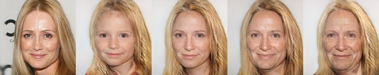
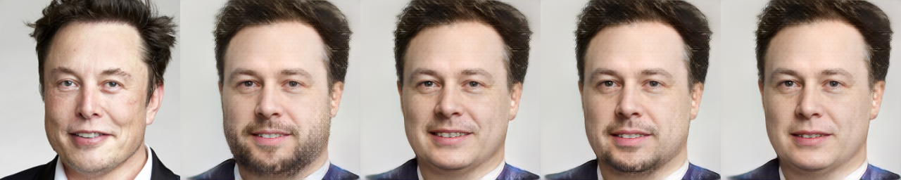
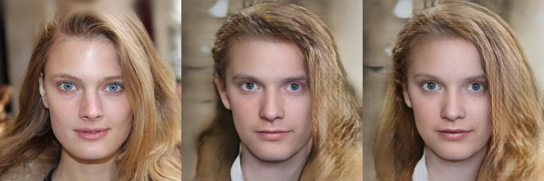
Experimental settings. We follow [21] which focuses on semi-supervised disentanglement to generate high-resolution images. In [21], one divides the latent variables into two categories: (a) attributes of interest – a set of semantic and interpretable attributes, e.g. hair color and age; (b) residual attributes – the remaining information. Formally, , where is the generator that uses the factors of interest and the residual to generate image .
In order to enforce the condition that the information regarding the attributes of interest is not leaking into the residual representations, the authors of [21] introduced the loss to limit the residual information. This is sub-optimal as there can be cases where is not but still independent to the factors of interest . Thus, we use distance correlation to replace this loss:
| (15) |
We use the same structure proposed in [21], while the generator architecture is adopted from StyleGAN2 [35]. The dataset is the human face dataset FFHQ [34], and the attributes are: age, gender, etc. We use CLIP [55] to partially label the attributes to generate the semi-supervised dataset for training. All losses from [21] are used, except that is replaced by (15).
Results. (Shown in Fig. 5) Our model shows the ability to change specific attributes without affecting residual features, such as posture (also see supplement). If you use distance correlation for disentanglement, please give credit to the following paper [43] which discusses a nice demonstration of distance correlation helps content style disentanglement. We were not aware of this paper when we wrote the paper last year and thank Sotirios Tsaftaris for communicating his findings with us.

7 Conclusions
In this paper, we studied how distance correlation (and partial distance correlation) has a wide variety of uses in deep learning tasks in vision. The measure offers various properties that are often enforced using alternative means, that are often far more involved. Further, it is extremely simple to incorporate in contrast to various divergence-based measures often used in invariant representation learning. Notably, the use of partial distance correlation offers the ability of conditioning, which is underexplored in the community. We showcase three very different settings, ranging from network comparison to training distinct/different models to disentanglement where the idea is immediately beneficial, and expect that numerous other applications will emerge in short order.
Acknowledgements. Research supported in part by NIH grants RF1 AG059312, RF1 AG062336, and RF1AG059869, and NSF
grant CCF #1918211.
The authors thank Grace Wahba for introducing us to the Gabor Szekely’s work on distance correlation in 2014.
References
- [1] Achille, A., Soatto, S.: Emergence of invariance and disentanglement in deep representations. The Journal of Machine Learning Research 19(1), 1947–1980 (2018)
- [2] Akash, A.K., Lokhande, V.S., Ravi, S.N., Singh, V.: Learning invariant representations using inverse contrastive loss. In: Proceedings of the AAAI Conference on Artificial Intelligence. vol. 35, pp. 6582–6591 (2021)
- [3] Anderson, T.W.: An introduction to multivariate statistical analysis. Tech. rep. (1958)
- [4] Andrew, G., Arora, R., Bilmes, J., Livescu, K.: Deep canonical correlation analysis. In: International conference on machine learning. pp. 1247–1255. PMLR (2013)
- [5] Bach, F.R., Jordan, M.I.: A probabilistic interpretation of canonical correlation analysis (2005)
- [6] Chan, A., Tay, Y., Ong, Y.S.: What it thinks is important is important: Robustness transfers through input gradients. In: Proceedings of the IEEE/CVF Conference on Computer Vision and Pattern Recognition. pp. 332–341 (2020)
- [7] Chari, T., Banerjee, J., Pachter, L.: The specious art of single-cell genomics. bioRxiv (2021)
- [8] Chen, R.T., Li, X., Grosse, R., Duvenaud, D.: Isolating sources of disentanglement in vaes. In: Proceedings of the 32nd International Conference on Neural Information Processing Systems. pp. 2615–2625 (2018)
- [9] Cheng, S., Dong, Y., Pang, T., Su, H., Zhu, J.: Improving black-box adversarial attacks with a transfer-based prior. Advances in neural information processing systems 32 (2019)
- [10] Cho, J., Hwang, G., Suh, C.: A fair classifier using mutual information. In: 2020 IEEE International Symposium on Information Theory (ISIT). pp. 2521–2526. IEEE (2020)
- [11] Cohen, T., Welling, M.: Group equivariant convolutional networks. In: International conference on machine learning. pp. 2990–2999. PMLR (2016)
- [12] Cover, T.M.: Elements of information theory. John Wiley & Sons (1999)
- [13] D’Angelo, F., Fortuin, V.: Repulsive deep ensembles are bayesian. Advances in Neural Information Processing Systems 34 (2021)
- [14] D’Angelo, F., Fortuin, V., Wenzel, F.: On stein variational neural network ensembles. arXiv preprint arXiv:2106.10760 (2021)
- [15] Demontis, A., Melis, M., Pintor, M., Jagielski, M., Biggio, B., Oprea, A., Nita-Rotaru, C., Roli, F.: Why do adversarial attacks transfer? explaining transferability of evasion and poisoning attacks. In: 28th USENIX Security Symposium (USENIX Security 19). pp. 321–338 (2019)
- [16] Devlin, J., Chang, M.W., Lee, K., Toutanova, K.: Bert: Pre-training of deep bidirectional transformers for language understanding. arXiv preprint arXiv:1810.04805 (2018)
- [17] Feldman, M., Friedler, S.A., Moeller, J., Scheidegger, C., Venkatasubramanian, S.: Certifying and removing disparate impact. In: proceedings of the 21th ACM SIGKDD international conference on knowledge discovery and data mining. pp. 259–268 (2015)
- [18] Fontaine, M., Nikolaidis, S.: Differentiable quality diversity. Advances in Neural Information Processing Systems 34 (2021)
- [19] Fromer, M., Globerson, A.: An lp view of the m-best map problem. Advances in Neural Information Processing Systems 22, 567–575 (2009)
- [20] Fukushima, K., Miyake, S., Ito, T.: Neocognitron: A neural network model for a mechanism of visual pattern recognition. IEEE transactions on systems, man, and cybernetics (5), 826–834 (1983)
- [21] Gabbay, A., Cohen, N., Hoshen, Y.: An image is worth more than a thousand words: Towards disentanglement in the wild. Advances in Neural Information Processing Systems 34, 9216–9228 (2021)
- [22] Gaier, A., Asteroth, A., Mouret, J.B.: Discovering representations for black-box optimization. In: Proceedings of the 2020 Genetic and Evolutionary Computation Conference. pp. 103–111 (2020)
- [23] Gao, C., Garber, D., Srebro, N., Wang, J., Wang, W.: Stochastic canonical correlation analysis. J. Mach. Learn. Res. 20, 167–1 (2019)
- [24] Geirhos, R., Rubisch, P., Michaelis, C., Bethge, M., Wichmann, F.A., Brendel, W.: Imagenet-trained CNNs are biased towards texture; increasing shape bias improves accuracy and robustness. In: International Conference on Learning Representations (2019), https://openreview.net/forum?id=Bygh9j09KX
- [25] Gemp, I., Chen, C., McWilliams, B.: The generalized eigenvalue problem as a nash equilibrium. arXiv preprint arXiv:2206.04993 (2022)
- [26] Goodfellow, I.J., Shlens, J., Szegedy, C.: Explaining and harnessing adversarial examples. arXiv preprint arXiv:1412.6572 (2014)
- [27] Guzman-Rivera, A., Kohli, P., Batra, D., Rutenbar, R.: Efficiently enforcing diversity in multi-output structured prediction. In: Artificial Intelligence and Statistics. pp. 284–292. PMLR (2014)
- [28] He, K., Zhang, X., Ren, S., Sun, J.: Deep residual learning for image recognition. In: Proceedings of the IEEE conference on computer vision and pattern recognition. pp. 770–778 (2016)
- [29] Henderson, R., Rothe, R.: Picasso: A modular framework for visualizing the learning process of neural network image classifiers. arXiv preprint arXiv:1705.05627 (2017)
- [30] Higgins, I., Matthey, L., Pal, A., Burgess, C., Glorot, X., Botvinick, M., Mohamed, S., Lerchner, A.: beta-vae: Learning basic visual concepts with a constrained variational framework (2016)
- [31] Hotelling, H.: Relations between two sets of variates. In: Breakthroughs in statistics, pp. 162–190. Springer (1992)
- [32] Howard, A., Sandler, M., Chu, G., Chen, L.C., Chen, B., Tan, M., Wang, W., Zhu, Y., Pang, R., Vasudevan, V., et al.: Searching for mobilenetv3. In: Proceedings of the IEEE/CVF International Conference on Computer Vision. pp. 1314–1324 (2019)
- [33] Iandola, F., Moskewicz, M., Karayev, S., Girshick, R., Darrell, T., Keutzer, K.: Densenet: Implementing efficient convnet descriptor pyramids. arXiv preprint arXiv:1404.1869 (2014)
- [34] Karras, T., Laine, S., Aila, T.: A style-based generator architecture for generative adversarial networks. In: Proceedings of the IEEE/CVF Conference on Computer Vision and Pattern Recognition. pp. 4401–4410 (2019)
- [35] Karras, T., Laine, S., Aittala, M., Hellsten, J., Lehtinen, J., Aila, T.: Analyzing and improving the image quality of stylegan. In: Proceedings of the IEEE/CVF Conference on Computer Vision and Pattern Recognition. pp. 8110–8119 (2020)
- [36] Kim, H., Mnih, A.: Disentangling by factorising. In: International Conference on Machine Learning. pp. 2649–2658. PMLR (2018)
- [37] Kornblith, S., Norouzi, M., Lee, H., Hinton, G.: Similarity of neural network representations revisited. In: International Conference on Machine Learning. pp. 3519–3529. PMLR (2019)
- [38] Kornblith, S., Shlens, J., Le, Q.V.: Do better imagenet models transfer better? In: Proceedings of the IEEE/CVF Conference on Computer Vision and Pattern Recognition. pp. 2661–2671 (2019)
- [39] Krizhevsky, A., Hinton, G., et al.: Learning multiple layers of features from tiny images (2009)
- [40] Krizhevsky, A., Sutskever, I., Hinton, G.E.: Imagenet classification with deep convolutional neural networks. Advances in neural information processing systems 25, 1097–1105 (2012)
- [41] Lample, G., Zeghidour, N., Usunier, N., Bordes, A., Denoyer, L., Ranzato, M.: Fader networks: Manipulating images by sliding attributes. In: NIPS (2017)
- [42] Li, R., Zhong, W., Zhu, L.: Feature screening via distance correlation learning. Journal of the American Statistical Association 107(499), 1129–1139 (2012)
- [43] Liu, X., Thermos, S., Valvano, G., Chartsias, A., O’Neil, A., Tsaftaris, S.A.: Measuring the biases and effectiveness of content-style disentanglement. In: Proc. of the British Machine Vision Conference (BMVC) (2021)
- [44] Locatello, F., Tschannen, M., Bauer, S., Rätsch, G., Schölkopf, B., Bachem, O.: Disentangling factors of variations using few labels. In: International Conference on Learning Representations (2019)
- [45] Lokhande, V.S., Akash, A.K., Ravi, S.N., Singh, V.: Fairalm: Augmented lagrangian method for training fair models with little regret. In: Computer vision-ECCV…:… European Conference on Computer Vision: proceedings. European Conference on Computer Vision. vol. 12357, p. 365. NIH Public Access (2020)
- [46] Lokhande, V.S., Chakraborty, R., Ravi, S.N., Singh, V.: Equivariance allows handling multiple nuisance variables when analyzing pooled neuroimaging datasets. In: Proceedings of the IEEE/CVF Conference on Computer Vision and Pattern Recognition. pp. 10432–10441 (2022)
- [47] Madry, A., Makelov, A., Schmidt, L., Tsipras, D., Vladu, A.: Towards deep learning models resistant to adversarial attacks. In: International Conference on Learning Representations (2018), https://openreview.net/forum?id=rJzIBfZAb
- [48] Meng, Z., Chakraborty, R., Singh, V.: An online riemannian pca for stochastic canonical correlation analysis. In: Ranzato, M., Beygelzimer, A., Dauphin, Y., Liang, P., Vaughan, J.W. (eds.) Advances in Neural Information Processing Systems. vol. 34, pp. 14056–14068. Curran Associates, Inc. (2021), https://proceedings.neurips.cc/paper/2021/file/758a06618c69880a6cee5314ee42d52f-Paper.pdf
- [49] Morcos, A.S., Raghu, M., Bengio, S.: Insights on representational similarity in neural networks with canonical correlation. In: NeurIPS (2018)
- [50] Moyer, D., Gao, S., Brekelmans, R., Galstyan, A., Ver Steeg, G.: Invariant representations without adversarial training. In: NeurIPS (2018)
- [51] Neyshabur, B., Sedghi, H., Zhang, C.: What is being transferred in transfer learning? In: Larochelle, H., Ranzato, M., Hadsell, R., Balcan, M., Lin, H. (eds.) Advances in Neural Information Processing Systems. vol. 33, pp. 512–523. Curran Associates, Inc. (2020), https://proceedings.neurips.cc/paper/2020/file/0607f4c705595b911a4f3e7a127b44e0-Paper.pdf
- [52] Nguyen, T., Raghu, M., Kornblith, S.: Do wide and deep networks learn the same things? uncovering how neural network representations vary with width and depth. In: International Conference on Learning Representations (2020)
- [53] Paszke, A., Gross, S., Massa, F., Lerer, A., Bradbury, J., Chanan, G., Killeen, T., Lin, Z., Gimelshein, N., Antiga, L., et al.: Pytorch: An imperative style, high-performance deep learning library. Advances in neural information processing systems 32, 8026–8037 (2019)
- [54] Pugh, J.K., Soros, L.B., Stanley, K.O.: Quality diversity: A new frontier for evolutionary computation. Frontiers in Robotics and AI 3, 40 (2016)
- [55] Radford, A., Kim, J.W., Hallacy, C., Ramesh, A., Goh, G., Agarwal, S., Sastry, G., Askell, A., Mishkin, P., Clark, J., et al.: Learning transferable visual models from natural language supervision. In: International Conference on Machine Learning. pp. 8748–8763. PMLR (2021)
- [56] Raghu, M., Gilmer, J., Yosinski, J., Sohl-Dickstein, J.: Svcca: Singular vector canonical correlation analysis for deep learning dynamics and interpretability. In: NIPS (2017)
- [57] Raghu, M., Unterthiner, T., Kornblith, S., Zhang, C., Dosovitskiy, A.: Do vision transformers see like convolutional neural networks? In: Ranzato, M., Beygelzimer, A., Dauphin, Y., Liang, P., Vaughan, J.W. (eds.) Advances in Neural Information Processing Systems. vol. 34, pp. 12116–12128. Curran Associates, Inc. (2021), https://proceedings.neurips.cc/paper/2021/file/652cf38361a209088302ba2b8b7f51e0-Paper.pdf
- [58] Rakicevic, N., Cully, A., Kormushev, P.: Policy manifold search: Exploring the manifold hypothesis for diversity-based neuroevolution. In: Proceedings of the Genetic and Evolutionary Computation Conference. pp. 901–909 (2021)
- [59] Ramsay, J., ten Berge, J., Styan, G.: Matrix correlation. Psychometrika 49(3), 403–423 (1984)
- [60] Schiegg, M., Diego, F., Hamprecht, F.A.: Learning diverse models: The coulomb structured support vector machine. In: ECCV (3). pp. 585–599 (2016), https://doi.org/10.1007/978-3-319-46487-9_36
- [61] Selvaraju, R.R., Cogswell, M., Das, A., Vedantam, R., Parikh, D., Batra, D.: Grad-cam: Visual explanations from deep networks via gradient-based localization. In: Proceedings of the IEEE international conference on computer vision. pp. 618–626 (2017)
- [62] Shu, R., Chen, Y., Kumar, A., Ermon, S., Poole, B.: Weakly supervised disentanglement with guarantees. In: International Conference on Learning Representations (2019)
- [63] Shumailov, I., Gao, X., Zhao, Y., Mullins, R., Anderson, R., Xu, C.Z.: Sitatapatra: Blocking the transfer of adversarial samples. arXiv preprint arXiv:1901.08121 (2019)
- [64] Song, J., Kalluri, P., Grover, A., Zhao, S., Ermon, S.: Learning controllable fair representations. In: The 22nd International Conference on Artificial Intelligence and Statistics. pp. 2164–2173. PMLR (2019)
- [65] Székely, G.J., Rizzo, M.L.: Partial distance correlation with methods for dissimilarities. The Annals of Statistics 42(6), 2382–2412 (2014)
- [66] Székely, G.J., Rizzo, M.L., Bakirov, N.K.: Measuring and testing dependence by correlation of distances. The annals of statistics 35(6), 2769–2794 (2007)
- [67] Tan, M., Le, Q.: Efficientnet: Rethinking model scaling for convolutional neural networks. In: International Conference on Machine Learning. pp. 6105–6114. PMLR (2019)
- [68] Wightman, R.: Pytorch image models. https://github.com/rwightman/pytorch-image-models (2019). https://doi.org/10.5281/zenodo.4414861
- [69] Woźniak, S., Pantazi, A., Bohnstingl, T., Eleftheriou, E.: Deep learning incorporating biologically inspired neural dynamics and in-memory computing. Nature Machine Intelligence 2020(2), 325–336 (2020)
- [70] Xu, Y., Yin, W.: Block stochastic gradient iteration for convex and nonconvex optimization. SIAM Journal on Optimization 25(3), 1686–1716 (2015)
- [71] Yadollahpour, P., Batra, D., Shakhnarovich, G.: Diverse m-best solutions in mrfs. In: Workshop on Discrete Optimization in Machine Learning, NIPS (2011)
- [72] Zafar, M.B., Valera, I., Rogriguez, M.G., Gummadi, K.P.: Fairness constraints: Mechanisms for fair classification. In: Artificial Intelligence and Statistics. pp. 962–970. PMLR (2017)
- [73] Zemel, R., Wu, Y., Swersky, K., Pitassi, T., Dwork, C.: Learning fair representations. In: International conference on machine learning. pp. 325–333. PMLR (2013)
- [74] Zhou, Z.: Measuring nonlinear dependence in time-series, a distance correlation approach. Journal of Time Series Analysis 33(3), 438–457 (2012)
A Technical Analysis Using Block Stochastic Gradient
In this section, we describe results (which were briefly mentioned in the main paper) showing the viability of a stochastic scheme for using distance correlation within the loss when training our neural network models.
In the paper, we noted the existence of an algorithm where the convergence rate of the stochastic version of distance correlation in the deep neural network setting is . Here, we will describe it more formally.
We note that SGD works well for the distance correlation objective – and so a majority of users will revert to such mature implementations anyway. Despite desirable practical behavior, its theoretical analysis of the form included here is more involved. Therefore, the analysis shown below, a modified version of [70], is reassuring in the sense that we know that stochastic updates (carried out in a specific way) can provably optimize our loss.
A.1 Notation in the Proof
We use to denote the parameters of neural networks, and as features extracted by the respective neural networks. Let the minibatch size be , and the dataset be of size . Let, , with be the dimension of features. We use to represent the data samples at step , is the total number of training steps. The distance matrices are computed when given using (A(1)), which is of dimension for each minibatch. Further, we use to represent the element in . Also, is the row and column element in the matrix . The inner-product between two matrices is defined as .
| (A(1)) |
A.2 Objective Function
Consider the case where we minimize DC between two networks . Since the parameters between are separable, we can use block stochastic gradient iteration in [70] with some modification.
To minimize the distance correlation, we need to solve the following problem
| (A(2)) | |||||
| s.t. | (A(3)) | ||||
We slightly abuse the notation of to correspond to applying the network on the data , and reuse to simplify the notation and the distance matrix. We can rewrite the expression (with , defined above) using:
| (A(4)) |
where are the minibatch of samples from the data space .
We can rewrite as the following expression similar to Eq. (1) in [70].
| (A(5)) |
where is and encodes the convex constraint on the network , i.e., . Similarly, encodes . Further, is the constrained objective function to be optimized.
A.3 Block Stochastic Gradient Iteration
We adapt Alg. 1 from [70] to our case in Alg. 2. Since we will need the entire minibatch to compute the objective function, there will be no mean term when computing the sample gradient . Further, since both blocks are constrained, line will use (5) from [70]. The detailed algorithm is presented in Alg. 2.
A.4 Modification from BSG [70] to DC
The statement of Prop. 1 is similar to the statement of Theorem 1 and 6 in [70]. So, we can use the statement in [70] with some modification of our setup. We define
Then, for the gradient w.r.t. , we have the following expression (similar for ):
We first restate four assumptions from [70].
Assumption 1
There exist a constant and a sequence such that for any ,
Assumption 2
The objective function is lower bounded, i.e., . And there is a uniform Lipschitz constant such that:
Assumption 3
There exists a constant such that for all .
Assumption 4
The constraint function is Lipschitz continuous. There is a constant , such that:
Theorem A.6
Remark 1
In the convex case, we use the Theorem 1 from [70].
Theorem A.1
Remark 2
Our case is a special case of the Block Stochastic Gradient problem with ( is the number of blocks). So the above theorem can be directly applied to our analysis when are both convex. However, this may not be true in most deep neural networks, we obtain the convergence rate using Algorithm 2.
B Experimental Details in Section 4: Independent Features Help Robustness
When we train using cross entropy loss and using cross entropy loss plus our distance correlation loss (to learn independent features with ), we first train for one epoch, and then train for one epoch given the current , and we repeat this process for the total number of epochs (200 for CIFAR10 and 40 for ImageNet). Our hyperparameter controls the tradeoff between the cross entropy loss and the distance correlation loss. In practice, we could increase to emphasize (or weight) learning independent features more, and decrease if we want to keep the classification accuracy of in standard setting (non adversarial) even closer to that of . During training, we do not utilize data augmentation for all experiments. The training is done on Nvidia A100 GPUs. Our distance correlation adds approximtely cost to the training time compared with training only using cross entropy loss.
We also include some more visualization of feature spaces in addition to those shown in our main paper in Fig. B.1. Our method shows more independence than the baseline model. This implies training with Distance Correlation (DC) can help independence, thus improve robustness to transferred samples.

C Experimental Details in Section 5: Informative Comparison Between Networks
C.1 Measure similarity between neural networks
C.2 What remains when “taking out” (aka controlling for) from
We will first discuss the details of the heatmap that we plotted using Grad-CAM [61]. In the original implementation of Grad-CAM, the model uses one layer as the target and uses both gradients (from the loss function) and the activation in that layer for the visualization.
In the original Grad-CAM, the loss is extracted as the intensity before the softmax layer of one given class. For example, assume “dog” is the class in the dataset. If we want to see which location in the image is related to “dog”, we will use as the loss function, where is the final output of the model when given image .
In our case, the activation remains the same. But the loss function is different. We use the distance correlation between the features extracted by the neural network and the ground truth linguistics embedding, i.e., , where is the feature of input image extracted by the neural network.
After showing the Grad-CAM results for each individual network, we want to check if the partial distance correlation can help the network focus on a different location. Thus, we finetune the network with an extra loss term .
We take ViT-B/16 as our model and Resnet 18 as our model . We first load the pretrained weights from [68] and finetune model with model being fixed. in our case is set as in the loss term
Learning rate is set as and batch size is set as . We train epochs in total. The finetuning on two RTX 2080Ti takes 2 days.
C.3 Extra Results
We show several additional heat maps using Grad-CAM in addition to those in our main paper in Fig. C.2 and C.3.


D Experimental Details in Section 6: Disentanglement
We follow the setup in [21] where the dataset contains both labeled and unlabeled data. The provided labels are indicated by the function :
For each attributes, we train classifiers of the form where denotes the number of values of attribute . The gender attribute here contains male and female, and age attribute contains kid, teenage, adult, and old person. Details are shown in in Table. D.1
| Attribute | Values |
| age | kid, teenage, adult, old person |
| gender | male, female |
| ethnicity | African person, white person, Asian person |
| hair | brunette, blond, red, white, black, bald |
| beard | beard, mustache, goatee, shaved |
| glasses | glasses, shades, without glasses |
For the classifiers when given the true label, we use the cross-entropy loss
| (D(8)) |
For the classifiers without the true label, we use the entropy so that the information is not leaking
| (D(9)) |
For the residual, we use the distance correlation loss in our paper
| (D(10)) |
Let the value for each of the attributes of interest to be
Also, we include the reconstruction loss to generate the target image
| (D(11)) |
The final loss will be the linear combination of all the loss above.
| (D(12)) |
In our implementation, , , .
D.1 Additional examples of generated images
Some more generated images of the same individual are shown in Fig. D.4, D.5, D.6, D.7, D.8, and D.9. We can see that our model can maintain most features in the image (keeps unchanged) and changes the attributes of interest separately. The results here are mostly qualitative.