On the universal constraints for relaxation rates for quantum dynamical semigroup

Introduction — Spectral analysis belongs to the heart of quantum theory [1]. Actually, this is spectroscopy which gave birth to quantum theory. Very often one infers information about the quantum system measuring a spectrum of some operator representing physical objects (quantum observables, quantum maps, etc.). In this Letter we analyze the spectral properties of the celebrated Gorini-Kossakowski-Lindblad-Sudarshan (GKLS) generator of quantum Markovian semigroup [2, 3]

where $\mathcal{L}$ has the following well known form

with arbitrary noise operators $L_{k}$ and positive rates $\gamma_{k}$. This is the most general structure of the generator which guaranties that the dynamical map $\Lambda_{t}=e^{t\mathcal{L}}$ is completely positive and trace-preserving (CPTP) [2, 3, 4, 5]. Solutions of (1) define very good approximation of real system’s evolution provided the system-environment interaction is sufficiently weak and there is separation of time scales for the system and environment [5]. Typical examples where Markovian approximation is physically justified are quantum optical systems [6, 7, 8]. It is well known that eigenvalues of $\mathcal{L}$ provide information about the rate of relaxation, dissipation and decoherence processes and hence define key physical property of the physical process. Actually, these are not $\gamma_{k}$ which are directly measured in the laboratory but the corresponding eigenvalues of the generator.

Let $\ell_{\alpha}$ be the corresponding (complex) eigenvalues of $\mathcal{L}$, that is, $\mathcal{L}(X_{\alpha})=\ell_{\alpha}X_{\alpha}$ for $\alpha=0,\ldots,d^{2}-1$, where $d={\rm dim}\,\mathcal{H}$. Since $\mathcal{L}$ does preserve Hermiticity one has $\mathcal{L}(X^{\dagger}_{\alpha})=\ell^{*}_{\alpha}X_{\alpha}^{\dagger}$, that is, if $\ell_{\alpha}$ is complex, then $\ell^{*}_{\alpha}$ is also an eigenvalue. It is well known [4] that $\lambda_{0}=0$ and the corresponding eigenvector (zero-mode of $\mathcal{L}$) $X_{0}$ gives rise to the invariant state of the evolution $\omega=X_{0}/{\rm Tr}\,X_{0}$, that is, $\Lambda_{t}(\omega)=\omega$. The corresponding eigenvalues $\lambda_{\alpha}(t)$ of the dynamical map $\Lambda_{t}=e^{t\mathcal{L}}$ read $\lambda_{\alpha}(t)=e^{t\ell_{\alpha}}$ and hence necessarily the relaxation rates $\Gamma_{\alpha}$ defined by

are non-negative $\Gamma_{\alpha}\geq 0$ for all $\alpha=1,\ldots,d^{2}-1$ (otherwise $e^{t\ell_{\alpha}}$ blows up as $t\to\infty$). Eigenvalues $\lambda_{\alpha}(t)$ of the corresponding dynamical map $\Lambda_{t}=e^{t\mathcal{L}}$ belong to the unit disc on the complex plane, that is, $|\lambda_{\alpha}(t)|\leq 1$. This is a quantum analog of the celebrated Frobenius-Perron theorem for stochastic matrices. Surprisingly, apart form the fact that all $\Gamma_{\alpha}\geq 0$ not much more is known about the structure of the spectrum of a GKSL generator. Actually, one can show that $e^{t\mathcal{L}}$ is CPTP for $t\geq 0$ if and only if $\mathcal{L}$ satisfy the following property (known as conditional complete positivity) [9, 10]

where $P=|\psi_{+}\rangle\langle\psi_{+}|$ denotes the projector onto maximally mixed state $|\psi_{+}\rangle\in\mathcal{H}\otimes\mathcal{H}$, and $P^{\perp}={\mathchoice{\rm 1\mskip-4.0mul}{\rm 1\mskip-4.0mul}{\rm 1\mskip-4.5mul}{\rm 1\mskip-5.0mul}}-P$ is orthogonal to $P$. Unfortunately, condition (4) does not provide any transparent information about the spectrum of $\mathcal{L}$. The same problem arises for quantum channels. A linear map $\Phi:\mathcal{B}(\mathcal{H})\to\mathcal{B}(\mathcal{H})$ is completely positive if and only if the corresponding Choi matrix $(I\otimes\Phi)(P)\geq 0$ [11]. Again, positivity of the Choi matrix cannot be easily translated into the property of the spectrum of the map $\Phi$. This should be clear since the map and hence also its Choi matrix depend in a nontrivial way both on the spectrum (eigenvalues) and eigenvectors. On the other hand eigenvalues and in particular relaxation rates have a clear physical interpretation and can be directly measured. Hence, eigenvalues of the Choi matrix decide about complete positivity and eigenvalues of the generator (or the quantum channel) are measurable quantities. It is, therefore, clear that one can expect some additional property relating relaxation rates which is responsible for complete positivity of the quantum evolution. Relaxation properties of GKLS generators were further studied in [4, 19] and more recently e.g. in [20, 21]. Some constraints for relaxation rates for 3- and 4-level systems were presented in [22, 23, 24]. Interestingly, authors of a seminal paper [2] already observed that for a qubit evolution governed by the following well known generator

with the dissipative part $\mathcal{L}_{D}=\gamma_{+}\mathcal{L}_{+}+\gamma_{-}\mathcal{L}_{-}+\gamma_{z}\mathcal{L}_{z}$ consisting of: pumping $\mathcal{L}_{+}(\rho)=\sigma_{+}\rho\sigma_{-}-\frac{1}{2}\{\sigma_{-}\sigma_{+},\rho\}$, damping $\mathcal{L}_{-}(\rho)=\sigma_{-}\rho\sigma_{+}-\frac{1}{2}\{\sigma_{+}\sigma_{-},\rho\}$, and dephasing $\mathcal{L}_{z}(\rho)=\sigma_{z}\rho\sigma_{z}-\rho$, complete positivity implies the following well known condition for the relaxation times $T_{\alpha}=1/\Gamma_{\alpha}$:

where the longitudinal rate $\Gamma_{\rm L}=\Gamma_{3}=\gamma_{+}+\gamma_{-}$, and transversal rate $\Gamma_{\rm T}=\Gamma_{1}=\Gamma_{2}=\frac{1}{2}(\gamma_{+}+\gamma_{-})+\gamma_{z}$. Condition (6) was experimentally demonstrated to be true [4, 12]. Clearly, the very condition (6) provides only partial information about the corresponding qubit generator. However, violation of (6) shows that the generator does not provide legitimate CPTP evolution. Condition (6) has even more appealing form when rephrased in terms of relaxation rates. Indeed, one finds

that is, each single relaxation rate cannot be too large. In terms of relative relaxation rates $R_{i}=\Gamma_{i}/(\Gamma_{1}+\Gamma_{2}+\Gamma_{3})$, it says that,

The generator (5) is very special and in particular implies that the rates $\Gamma_{1}$ and $\Gamma_{2}$ are the same. Interestingly, Kimura [13] showed that condition (7) is universal for any qubit generator. For a purely dissipative generator Wolf and Cirac derived the following result (Theorem 6 in [14])

with $\Gamma:=\sum_{\beta=1}^{d^{2}-1}\Gamma_{\beta}$, where $\|\mathcal{L}\|$ denotes the operator norm. Note, that due to $\|\mathcal{L}\|\geq|\ell_{\alpha}|\geq\Gamma_{\alpha}$, the above condition implies

where $R_{\alpha}=\Gamma_{\alpha}/\Gamma$. Recently, Kimura et al. [15] obtained the following universally valid constraints for any GKLS generator:

In this Letter we conjecture that the bound (11) can be still improved and propose the following

Unfortunately, we still do not have a complete proof of (12). However, we show in this Letter that this conjecture holds for several important classes of GKLS generators. In particular any generator giving rise to the unital evolution, that is $\mathcal{L}({\mathchoice{\rm 1\mskip-4.0mul}{\rm 1\mskip-4.0mul}{\rm 1\mskip-4.5mul}{\rm 1\mskip-5.0mul}})=0$, satisfies (12). Unital (often called doubly stochastic) maps characterize decoherence processes that does not decrease entropy [25, 26] and provide direct generalization of unitary maps. A second important class are GKLS generator which display additional symmetry, that is, they are covariant w.r.t. maximal abelian subgroup of the unitary group $U(d)$. Actually, qubit generator (5) belongs to this class. The classical Pauli master equation is another example.

The formula (2) provides the most general mathematical structure of the generator compatible with the requirement of complete positivity and trace-preservation. Note, however, that not every generator constructed according to (2) has a clear physical interpretation. There exists a natural class of generators of Markovian semigroups derived in the weak coupling limit [17, 4, 5] and these do enjoy the covariance property. Hence, we may summarise that physically motivated generators do satisfy Conjecture (1). This conjecture is also strongly supported by numerical analysis (cf. Figure 1).

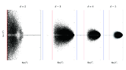
Interestingly, it is perfectly consistent with the spectrum of random GKLS generator in the large $d$-limit [16]. Finally, we also construct a GKLS model which saturates (13) (for some $\alpha$). This implies that (13) are the tightest constraints which characterize the universally valid spectral property of GKLS generators.

Clearly, the conjecture providing universal constraints for relaxation rates is interesting by itself since they are composed of experimentally accessible quantities and hence provide a direct method to check the validity of GKLS generators, or the completely positive condition. It has, however, further very interesting implications. It allows to establish universal constraints for eigenvalues of quantum channels (Conjecture 2). Moreover, it provides necessary condition for a quantum channel $\Phi$ to be represented via $\Phi=e^{\mathcal{L}}$ for some GKLS generator [9]. It is found that in this case all eigenvalues are constrained to a ring $r\leq|z_{\alpha}|\leq 1$, where the inner radius $r$ is fully characterized by the original channel $\Phi$ (Conjecture 3).

where $K$ is the classical generator satisfying the following Kolmogorov conditions [27]

Hence $K_{ij}$ can be represented as $K_{ij}=t_{ij}-\delta_{ij}\sum_{m=1}^{d}t_{mj}$, with $t_{ij}\geq 0$. Note that here only $t_{ij}$ with $i\neq j$ are relevant, so in the following, we put $t_{ii}=0$. Equivalently, (14) can be formulated as follows

Do we have a classical analog of (12)? Spectral properties of $d\times d$ matrix $K_{ij}$ are similar to that of $\mathcal{L}$: there are $d$ complex eigenvalues $\ell^{\rm cl}_{0},\ldots,\ell^{\rm cl}_{d-1}$ with $\ell^{\rm cl}_{0}=0$. Moreover, $\Gamma^{\rm cl}_{k}=-{\rm Re}\,\ell^{\rm cl}_{k}\geq 0$, and the spectrum is symmetric w.r.t. real axis. Interestingly, in the classical case there is no bound on the relative classical rates $R^{\rm cl}_{k}$, that is, given a set of classical rates $\Gamma^{\rm cl}_{k}\geq 0$ one can construct a classical generator $K_{ij}$ which does display exactly these rates. In particular any single relative rate $R^{\rm cl}_{k}$ can be arbitrary close to ‘$1$’. (See Appendix A for details.)

Consider now a quantum evolution $t\to\rho(t)$ such that the diagonal elements $p_{k}=\rho_{kk}$ evolve according to the classical Pauli equation (14). Introducing the family of noise operators $E_{ij}=|i\rangle\langle j|$ one constructs the following GKLS generator

where $B=\sum_{k}b_{k}|k\rangle\langle k|$, with $b_{k}=\sum_{j=1}^{d}t_{jk}$. The spectrum of $\mathop{\mathcal{L}}\nolimits$ consists of $d$ classical eigenvalues of the classical generator represented by the matrix $K_{ij}=t_{ij}-\delta_{ij}b_{j}$: $\lambda_{0}=0,\ell^{\rm cl}_{1},\ldots,\ell^{\rm cl}_{d-1}$, and the remaining eigenvalues correspond to eigenvectors $E_{kl}$:

Hence, one has classical rates $\Gamma^{\rm cl}_{1},\ldots,\Gamma^{\rm cl}_{d-1}$, and the remaining quantum rates

For the proof see Appendix B. This simple analysis shows that the role of quantum rates $\Gamma_{kl}$ is to restore the bound (12) which is violated if one considers only classical rates $\Gamma^{\rm cl}_{k}$. In terms of relative rates for the original classical problem $R^{\rm cl}_{k}$ can be arbitrarily close to ‘$1$’. However, after incorporating the remaining rates $\Gamma_{kl}$ one finds

Clearly, this is the requirement of complete positivity which enforces the rates to satisfy (12).

for some Hermitian operator $\Sigma$. A well known example is a qubit dephasing corresponding to $\Sigma=\sigma_{z}$. Let $\Sigma=\sum_{k}s_{k}|k\rangle\langle k|$ and assume that $s_{1}\leq\ldots\leq s_{d}$. Then one finds for the relaxation rates $\Gamma_{ij}=(s_{i}-s_{j})^{2}$ with the maximal rate $\Gamma_{\rm max}=\Gamma_{1d}$. One shows (cf. Appendix C) that

which supports the conjecture (12). Moreover, taking $s_{2}=\ldots=s_{d-1}=\frac{s_{1}+s_{d}}{2}$, one finds $\sum_{i,j=1}^{d}\Gamma_{ij}=d\Gamma_{\rm max}$, or equivalently $R_{\rm max}=\frac{1}{d}$.

for all $X\in\mathcal{B}(\mathcal{H})$. Inserting the formula (2) for the generator one finds (cf. Appendix D)

Now, inserting $X=Y_{\alpha}$, where $\mathcal{L}^{\ddagger}(Y_{\alpha})=\ell_{\alpha}Y_{\alpha}$ one obtains

which finally implies

where $\omega$ is an invariant state satisfying $\mathcal{L}(\omega)=0$. One has therefore

and hence one finds the following formula for $\Gamma_{\alpha}$

Introducing the following inner product $(A,B)_{\omega}={\rm Tr}(\omega A^{\dagger}B)$ and the corresponding $\omega$-norm $\|A\|_{\omega}^{2}=(A,A)_{\omega}$ the formula (24) may be rewritten in the following compact form

This formula is universal, that is, it holds for any GKLS generator. Clearly, to compute $\Gamma_{\alpha}$ one has to know the corresponding eigenvector $Y_{\alpha}$ and the invariant state $\omega$. In particular, since $Y_{0}={\mathchoice{\rm 1\mskip-4.0mul}{\rm 1\mskip-4.0mul}{\rm 1\mskip-4.5mul}{\rm 1\mskip-5.0mul}}$, one recovers $\Gamma_{0}=0$.

Inserting $\omega={\mathchoice{\rm 1\mskip-4.0mul}{\rm 1\mskip-4.0mul}{\rm 1\mskip-4.5mul}{\rm 1\mskip-5.0mul}}/d$ into formula (25) one obtains

where now $\|A\|^{2}={\rm Tr}(A^{\dagger}A)$. To prove (12) we use the following intricate inequality [28]

Actually, this inequality was conjectured by Böttcher and Wenzel [29] in 2005 (see [28] for more details). A simpler proof can be found in [30]. It should be stressed that the bound (11) was shown by the direct use of this inequality as well.

Now, (29) immediately implies

Assuming the following normalization $\|L_{k}\|^{2}=1$ as well as the condition $\mathrm{Tr}L_{k}=0$ without loss of generality, one shows (cf. Appendix E) that

and hence (30) reproduces (12). Thus, we have shown

where $U_{\mathbf{x}}=\sum_{k=1}^{d}e^{-ix_{k}}|k\rangle\langle k|$, and $\mathbf{x}=(x_{1},\ldots,x_{d})\in\mathbb{R}^{d}$. Any generator satisfying (32) has the following form

where $\mathop{\mathcal{L}}\nolimits_{0}(\rho)=-i[H,\rho]$, together with

where the Hamiltonian $H=\sum_{i}h_{i}|i\rangle\langle i|$, $B=\sum_{j}b_{j}|j\rangle\langle j|$, with $b_{j}=\sum_{i}t_{ij}$, and $D=\sum_{i=1}^{d}d_{ii}|i\rangle\langle i|$ (See Appendix F). This is GKLS generator iff $t_{ij}\geq 0$ and the Hermitian matrix $[d_{ij}]_{i,j=1}^{d}$ is positive definite. Clearly, $\mathop{\mathcal{L}}\nolimits_{1}$ is a classical generator considered before and $\mathop{\mathcal{L}}\nolimits_{2}$ adds pure decoherence with respect to the orthonormal basis $|1\rangle,\ldots,|d\rangle$. Interestingly, the very condition (32) implies that $\mathop{\mathcal{L}}\nolimits_{\alpha}\,\mathop{\mathcal{L}}\nolimits_{\beta}=\mathop{\mathcal{L}}\nolimits_{\beta}\,\mathop{\mathcal{L}}\nolimits_{\alpha}$ for $\alpha=0,1,2$. Hence $\mathop{\mathcal{L}}\nolimits_{0},\mathop{\mathcal{L}}\nolimits_{1},\mathop{\mathcal{L}}\nolimits_{2}$ share the same eigenvectors. It is, therefore, clear that eigenvalues of $\mathcal{L}$ are simply sum of eigenvalues of $\mathop{\mathcal{L}}\nolimits_{\alpha}$. Due to this property the analysis of $\mathcal{L}$ leads to the following

For the proof see Appendix G.

Since the Conjecture 1 holds in the qubit case one has

Indeed, (36) follows immediately from (35) for $d=2$. In particular for the Pauli channel $\Phi(\rho)=\sum_{\alpha=0}^{3}p_{\alpha}\sigma_{\alpha}\rho\sigma_{\alpha}$ one has $z_{k}=x_{k}$, and (36) are equivalent to the celebrated Fujiwara-Algoet conditions [41]. Moreover, since the Conjecture 1 holds for generators satisfying $\mathcal{L}({\mathchoice{\rm 1\mskip-4.0mul}{\rm 1\mskip-4.0mul}{\rm 1\mskip-4.5mul}{\rm 1\mskip-5.0mul}})=0$, one immediately proves

A second immediate implication of Conjecture 1 is the problem of deciding whether a given quantum channel $\Phi$ can be represented as $\Phi=e^{\mathcal{L}}$ for some GKLS generator $\mathcal{L}$ [9, 14]. Our original Conjecture 1 implies

Interestingly, it shows that all $z_{\alpha}$ are not only constrained to the unit Frobenius disc but belong to the ring

Clearly, Conjecture 3 is satisfied for all qubit channels and all unital channels. In particular for a qubit Pauli channel all eigenvalues $z_{\alpha}$ are real and hence (37) reduces to the following simple condition $z_{i}z_{j}\leq z_{k}$, where $i,j,k\in\{1,2,3\}$ are all different. This condition was recently derived in [33, 34].

References

- [1] J. von Neumann, Mathematical Foundations of Quantum Mechanics (Princeton University Press, New Jersey, 1955).
- [2] V. Gorini, A. Kossakowski, and E. C. G. Sudarshan, J. Math. Phys. 17, 821 (1976).
- [3] G. Lindblad, Comm. Math. Phys. 48, 119 (1976).
- [4] R. Alicki and K. Lendi, Quantum Dynamical Semigroups and Applications (Springer, Berlin, 1987).
- [5] H.-P. Breuer and F. Petruccione, The Theory of Open Quantum Systems (Oxford Univ. Press, Oxford, 2007).
- [6] C. W. Gardiner and P. Zoller, Quantum Noice, Springer-Verlag, Berlin, 1999.
- [7] M. B. Plenio and P. L. Knight, Rev. Mod. Phys. 70, 101 (1998).
- [8] H. J. Carmichael, Statistical Methods in Quantum Optics I: Master Equations and Fokker-Plack Equations, (Berlin: Springer 1999).
- [9] M. M. Wolf, J. Eisert, T. S. Cubitt, J. I. Cirac, Phys. Rev. Lett. 101, 150402 (2008).
-
[10]
M. M. Wolf, Quantum Channels & Operations: Guided Tour, URL: https://wwwm5.ma.tum.de/foswiki/pub/M5/Allgemeines
/MichaelWolf/QChannelLecture.pdf. - [11] M.-D. Choi. Lin. Alg. Appl. 10, 285 (1975).
- [12] A. Abragam, Principles of Nuclear Magnetism (Oxford University Press, 1961); C. P. Slichter, Principles of Magnetic Resonance (Springer-Verlag, 1990).
- [13] G. Kimura, Phys. Rev. A 66, 062113 (2002).
- [14] M. M. Wolf and I. Cirac, Comm. Math. Phys. 279, 147 (2008).
- [15] G. Kimura, S. Ajisaka, K. Watanabe, Open Syst. Inform. Dynam. 24(4): 1-8 (2017).
- [16] S. Denisov, T. Laptyeva, W. Tarnowski, D. Chruściśski, and K. Życzkowski, Phys. Rev. Lett. 123, 140403 (2019).
- [17] E. B. Davies, Commun. Math. Phys. 39, 91 (1974).
- [18] E. B. Davies, Quantum Theory of Open Systems. (Academic Press, New York) 1976.
- [19] H. Spohn, Rev. Mod. Phys. 52, 569 (1980).
- [20] K. Dietz, J. Phys. A: Math. Gen. 37, 6143 (2004).
- [21] B. Baumgartner, H. Narnhofer, and W. Thirring, J. Phys. A: Math. Gen. 41, 065201 (2008).
- [22] S. G. Schirmer and A. I. Solomon, Phys. Rev. A 70, 022107 (2004).
- [23] P. R. Berman and R. C. O’Connell, Phys. Rev. A 71, 022501 (2005).
- [24] D. K. L. Oi and S. G. Schirmer, Phys. Rev. A 86, 012121 (2012).
- [25] F. Benatti, Lett. Math. Phys. 15, 325 (1988).
- [26] P. Aniello, D. Chruściński, J. Phys. A: Math. Gen. 49, 345301 (2016).
- [27] N. G. van Kampen, Stochastic Processes in Physics and Chemistry, North Holland, Amsterdam 2007.
- [28] A. Böttcher and D. Wenzel, Lin. Alg. Appl. 429, 1864 (2008);
- [29] A. Böttcher and D. Wenzel, Lin. Alg. Appl. 403, 216 (2005).
- [30] K. Audenaert, Lin. Alg. Appl. 432, 1126 (2010).
- [31] F. Benatti and R. Floreanini, Mod. Phys. Lett. A 12, 1465 (1997).
- [32] A. Rivas and S. F. Huelga, Open Quantum Systems. An Introduction (Springer, Heidelberg, 2011).
- [33] D. Davalos, M. Ziman, and C. Pineda, Quantum 2, 144 (2019).
- [34] Z. Puchała, L. Rudnicki, and K. Życzkowski, Phys. Lett. A 383, 2376 (2019).
- [35] Á. Rivas, S. F. Huelga, and M. B. Plenio, Rep. Prog. Phys. 77, 094001 (2014).
- [36] H.-P. Breuer, E.-M. Laine, J. Piilo, and B. Vacchini, Rev. Mod. Phys. 88, 021002 (2016).
- [37] I. de Vega and D. Alonso, Rev. Mod. Phys. 89, 015001 (2017).
- [38] L. Li, M. J.W. Hall, and H. M. Wiseman, Phys. Rep. 759, 1 (2018).
- [39] Á. Rivas, S.F. Huelga, and M.B. Plenio, Phys. Rev. Lett. 105, 050403 (2010).
- [40] D. Chruściński and S. Maniscalco, Phys. Rev. Lett. 112, 120404 (2014).
- [41] A. Fujiwara and P. Algoet. Affine parameterization of completely positive maps on a matrix algebra. Phys. Rev. A 59, 3290 (1999).
- [42] J. Watrous, The Theory of Quantum Information, (Cambridge University Press, 2018)