On the topological character of three-dimensional Nexus triple point degeneracies
Abstract
Recently a generic class of three-dimensional band structures was identified that host two-fold line degeneracies meeting at three-fold or triple point degeneracies, which resist the usual topological characterization of isolated point degeneracies as in Dirac/Weyl semimetals. For these so-called “Nexus” fermions which lie beyond Dirac/Weyl fermions, we lay out several concepts to characterize the wavefunction geometry and spell out its topology. Our approach is based on an understanding of the analyticity properties of Nexus wavefunctions building on a two-dimensional analogue studied recently by us. We use this to write down a homological characterization of various Nexus triple point degeneracies in three dimensions.
I Introduction
Band theory of electronic structure occupies a venerable place in quantum condensed matter. Historically, the basic ideas were established quite soon after the development of quantum mechanics. Yet, it is still an active area of research with many surprises. Among the surprises, topological band insulators and superconductors have captured our imagination in a big way. Hasan and Kane (2010) They had their antecedent in the integer quantum Hall effect. Thouless et al. (1982); Klitzing et al. (1980) The electronic structure of these quantum states of matter have interesting and robust phenomenology, e.g. the edge states of topological bands. Wen (1991); Hasan and Kane (2010) Another surprise has been the wealth of physics present in two and three dimensional ( and ) semimetals. Vafek and Vishwanath (2014); Armitage et al. (2018) The low energy excitations in semimetals also often possess a topological character. This can lead to a certain robustness against back-scattering. Wehling et al. (2014) Already the low density of semimetallic carriers at the Fermi energy makes the effect of interactions less relevant. The combination of these two effects holds promise for technological applications of semimetals. Yan and Felser (2017)
From a theoretical point of view, what gives the semimetallic carriers their topological character is the global structure of their wavefunction geometry in the Brillouin zone. Dirac and Weyl semimetals are the well-known examples in and . These semimetals have two-fold degeneracies (not counting spin) at isolated points in the Brillouin zone often protected by certain symmetries. Vafek and Vishwanath (2014); Das et al. (2020) They can be thought as “topological defects” in the space of the band wavefunctions. The semimetallic character obtains when the Fermi energy is near these degeneracies. Such two-fold point degeneracies are generic only in , while they are exceptional in thus requiring symmetry protection. von Neuman and Wigner (1929) Recently, generalization of Dirac and Weyl fermions have also been found by symmetry-protecting higher-fold point degeneracies. Bradlyn et al. (2016)
While there has been tremendous activity on semimetals with point degeneracies, it has also been realized that band structures with two-fold line degeneracies are another possibility in the universe of possible band structures. Line degeneracies are exceptional in , and symmetry protection is required to obtain them. Several symmetry protected possibilities have been identified recently. Burkov et al. (2011); Phillips and Aji (2014); Zhu et al. (2016); Chang et al. (2017) Among these, there is a class of band structures where two-fold line degeneracies meet at three-fold or triple point degeneracies. They have been dubbed as Nexus fermions. Chang et al. (2017); Heikkilä and Volovik (2015) There have been material proposals Chang et al. (2017); Zhang et al. (2017); Feng et al. (2018); Weng et al. (2016a, b); Hyart and Heikkilä (2016) and experimental observations Lv et al. (2017); Ma et al. (2018) on this class of fermions. Their spectral structure is intriguing, and their band topology has been analysed previously in terms of the line degeneracies and topological numbers. Winkler et al. (2019) The goal of this paper is to shed more light on the band topology of Nexus fermions in a different manner which particularly emphasizes Nexus triple points themselves. We want to characterize the topology of these triple point degeneracies when thought of as defects in the space of band wavefunctions.
The topological character of point degeneracies can be understood by studying the band topology in one lower dimension. Schnyder et al. (2008) One generally considers a surface in the momentum space that encloses the point degeneracy in question. Since the surface can be chosen to be gapped everywhere, one then computes the Chern number on this surface which serves as a topological charge for the point degeneracy. This discrete topological charge can not be changed by small deformations to the Hamiltonian. This approach will fail to characterize a Nexus triple point degeneracy, because any surface enclosing it will have gapless points where the line degeneracies intersect with the chosen surface. Thus the general principle of calculating a topological charge on an enclosing surface will not work. This is why Ref. Chang et al., 2017 called Nexus fermions as “beyond-Weyl”. If we restrict ourselves to use only gapped lower dimensional spaces, one can characterize the topology of the line degeneracies by considering gapped loops around them. Heikkilä and Volovik (2015); Zhu et al. (2016); Winkler et al. (2019) Also, one can enclose two or more different triple points together by a gapped surface in some cases and calculate a topological invariant on that surface. Zhu et al. (2016)
The question then is how to proceed in order to characterize the band topology of a Nexus system. This includes the basic issue of whether Nexus triple points have a topological character or not. This is a relevant question not just as a conceptual issue, but also because of the following physical point: in Weyl systems, the surface Fermi arcs have a protection in the sense that they have to end at the projection of the bulk Weyl points on to the surface. Armitage et al. (2018) This protection is linked to the fact that the Weyl points in the bulk possess a topological character. Ref. Chang et al., 2017 raised the analogous question on whether the surface Fermi arcs numerically observed in their chosen Nexus systems have a topological protection in the sense of Weyl Fermi arcs. See the discussion on the Nexus Fermi arcs in Ref. Chang et al., 2017 for more on this point. Our paper gives a constructive method to capture the topological character of different Nexus triple points. This method is the main result of this paper. Thus, we give an affirmative answer to the question raised in Ref. Chang et al., 2017, i.e. there will be surface Fermi arcs in Nexus systems that will have to end at the projection of the bulk triple points on to surface. We note here that Ref. Zhu et al., 2016 give an alternate argument for the presence of protected Fermi arcs in these systems based on mirror Chern numbers Teo et al. (2008) without concerning directly with the topological character of the Nexus points.
Our method relies crucially on the analytic properties of the band wavefunctions near the line degeneracies. This builds on the results of Ref. Das and Pujari, 2019 where a toy band structure was considered which had a certain likeness to the Nexus band structures. In particular, specific cuts of some Nexus band structure resembles the toy band structure considered in Ref. Das and Pujari, 2019. The wavefunctions of this toy model were written down which made the band topology explicit. The topology could be captured by a generalization of winding numbers. Park and Marzari (2011); Das and Pujari (2019) This taught us the bigger lesson that near line degeneracies, analytic continuation or movement in the space of wavefunctions is key to exposing the band topology even in .
Motivated by the above, we will study in detail the analyticity properties of several Nexus band structures. We will use Dirac and Weyl systems as scaffolding for the analyticity discussions of Nexus band structures. In the process, we will come to an important notion of the generalized domain when dealing with degeneracies. This will be necessitated by the presence of degenerate points on the surface enclosing the Nexus triple point degeneracy. For point degeneracies like Weyl points, this notion is not necessitated because we can easily find a gapped surface to surround the Weyl point.
Equipped with the generalized domain, we can finally state data on the band topology of a Nexus band structure. This scheme will consist of specifying and counting the distinct analytic loops that can be drawn on the generalized domain around a triple point. Thus we will have the desired scheme to distinguish different triple point degeneracies based on their distinct band topology data. This idea is very similar to the homology classes of 1-cycles used to distinguish the topology of different geometric objects. Nakahara (2003) The familiar example is that of a sphere vs. a torus. The sphere admits no loops that can’t be contracted to a point, whereas a torus admits two distinct classes of loops that can’t be contracted to a point. Our scheme will do a similar characterization of the triple points, with the structure of the homology classes being dictated by the structure of the line degeneracies. In this way, we will be able to describe several Nexus band structures written down in the literature Chang et al. (2017) as well as some obtained as extensions of the toy band structure in Ref. Das and Pujari, 2019. This is the culminating result of this paper. Furthermore, this scheme can also potentially reveal the inter-relationships between different kinds of triple points.
We give a brief outline of the paper: Sec. II sets the stage by recapitulating some band structures from the point of view of analyticity. We will be paying close attention to what happens near degeneracies, since that is the main roadblock in understanding the band topology of Nexus band structures. Doing this will introduce the notion of the generalized domain. We then go on in Sec. III. We start by discussing the familiar Weyl system to give a clear contrast to Nexus band structures in terms of their analyticity properties. We then discuss several Nexus band structures. Sec. IV will finally give the method to state the band topology data in terms of homology classes of analytic loops on a generalized domain around the triple point. This won’t be hindered by a lack of gapped property, because analyticity near the degeneracies constrain the wavefunctions enough to enable stating the topology. This will conclude our exposition on the band topology of Nexus fermions. We end the paper in Sec. V with a summary and outlook. We also discuss here our take on the Fermi arc phenomenology of Nexus systems including a conjecture regarding the charge of these surface states.
II 2D Analyticity
In this section, we will start with the analyticity discussion in a beyond-Dirac Nexus system. Let’s reconsider the band structure introduced in Ref. Das and Pujari, 2019 to set up the discussion:
| (1) |
The eigensystem of is
| (2a) | ||||
| (2b) | ||||
where . , are the complex cube roots of unity and . This band structure possesses a three-fold degeneracy at clearly, and has two line degeneracies coming out from the triple point which is a signature feature of Nexus wavefunctions. Because of the line degeneracies, a standard Berry phase description of the wavefunction geometry is not applicable. However, we had used generalized winding numbers Das and Pujari (2019); Park and Marzari (2011) to understand this wavefunction geometry (cf. Table I and Sec. II of Ref. Das and Pujari, 2019) and contrasted with other known Dirac-like wavefunction geometries. In , such winding number description is not generally applicable for classification of point degeneracies. Thus, we will take the approach to be described below and in future sections.
Our main point of view will be to understand and write down the key aspects of the analytic behavior of various band structures. This is a different way of communicating invariant data of the wavefunction geometry than winding numbers and Berry phases. For example, we often view the familiar two-fold Dirac system
| (3) |
with the eigensystem as
| (4) |
by calculating Berry phase or chiral winding number Ryu et al. (2010); Schnyder et al. (2008) on gapped region in one lower dimension (e.g. any closed loop around the degeneracy). We rather want to include the degeneracy to be a part of the analysis.
Firstly, on a gapped loop we clearly have the analyticity property
| (5) |
However, we also have the following analyticity property of Dirac wavefunctions
| (6) |
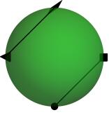
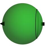
which connects the two bands. In fact, this relation tells us how to consistently arrive at the two-fold degeneracy from all sides without running into analytic ambiguities. Thus, we can interpret this as the way to move analytically across the point degeneracy. This is illustrated in the two figures from the left in Fig. 1.


Eq. 5 and 6 are nothing but an alternate way of describing the wavefunction geometry that is captured by Berry phase and chiral winding numbers, with the additional benefit of allowing to move across the degeneracy in an analytically smooth way. This alternate viewpoint will prove useful for us because Nexus triple points can not be enclosed by a gapped region in one lower dimension. As notation, we refer to analyticity relations with the same band index on left and right hand sides as “index-preserving” (e.g. Eq. 5), while analyticity relations with different band indices on both sides as “index-connecting” (e.g. Eq. 6).
For a quadratic band touching (QBT), the analyticity relation is in fact
| (7) |
We can understand this in terms of two Dirac points (of same winding) sitting on top of each other. Let’s first imagine these two Dirac points are not on top of each other, and we move analytically across both the degeneracies in a single go. In this process, we will return back to the same band that we started from as illustrated in Fig. 2. Now, imagine moving these two Dirac points till they fall on top of each other to obtain a QBT. Analyticity thus forces us that we will stay in the same band when we cross the QBT (bottom panel of Fig. 2), i.e. Eq. 7. This argument also works when the QBT splits into more Dirac points, e.g. in Bernal-stacked honeycomb bilayer lattice in presence of “trigonal” warping terms when it splits into three Dirac points of same winding and a fourth one with opposite winding. Mikitik and Sharlai (2008)


With the above discussion in hand, we can revisit the system in Eq. 1 and 2 in terms of its key analyticity information. The index-connecting relation is
| (8) |
which may be contrasted with Eq. 6 in the Dirac case. Similarly, in contrast to Eq. 5, we arrive at the index-preserving relation
| (9) |
This unusual “” structure is a result of the Nexus lines emanating from the three-fold degeneracy. We emphasize that the above two relations are an alternate way of describing the wavefunction geometry when compared to a generalized winding number description. Das and Pujari (2019) This way of stating the wavefunction geometry via the analyticity will be our approach to tackle the Nexus geometry in the next sections.
We end this section with a final conceptual point. Even though Eq. 1 and 3 are multi-band systems as expressed through band-indexed eigenfunctions in Eq. 2 and 4, the analytic structure actually tells us that this band distinction is a matter of convenience or convention and not fundamental when considering the wavefunction geometry. We can imagine a single function defined on a generalized domain that describes the multi-band wavefunctions in analogy with Riemann surfaces. This analogy can be made exact for Eq. 2 by re-writing as , whereby we can essentially drop the index to write as , that is defined on a three-fold Riemann surface connected by branch cuts of the complex cube root function. This generalized domain restatement succinctly tells us how to analytically move in the space of wavefunctions, which is of course a key requirement to understand the wavefunction geometry.
A similar generalized domain restatement can be done for the case of Dirac eigensystem Eq. 4. The generalized domain is composed of two copies of the - plane connected at the point-degeneracy. The band-connection relation (Eq. 6) gives us the rule of moving through the “connecting point” in the generalized domain from one copy of the - plane to the other (see the rightmost figure of Fig. 1). In the Dirac case, there is no branch cut structure since the eigensystem (Eq. 4) is perfectly analytic. The generalized domain will be used when we discuss the Nexus wavefunctions in the next sections.
III 3d Analyticity
In this section, we start with the actual discussion on the analyticity properties of Nexus fermions. As mentioned in Sec. I, line degeneracies are exceptional in and require symmetry protection, whereas they are fine-tuned in . Thus the analyticity discussion in the previous section is for a fine-tuned case, but it will help us in the following discussions. Before we go towards Nexus analyticity properties, let us start with the familiar case of Weyl point degeneracies to set the stage.
III.1 Weyl analyticity
A Weyl point degeneracy is characterized by an effective (low-energy) Hamiltonian of the form . The eigenenergies are , and the eigenfunctions are generally expressed as
| (10a) | ||||
| (10b) | ||||
In our gauge choice where the last term is kept purely real, they are
| (11a) | ||||
| (11b) | ||||
Often, the wavefunction geometry of point degeneracies are understood by considering a surface enclosing the point degeneracy and computing the Chern number of the two gapped bands on this reduced system. For the Weyl system, the Chern number of the two gapped bands are . We note that in the full BZ, the number of Weyl points has to be even such that the sum of their Chern numbers is zero, as the Chern number computed on the BZ boundary must be zero by periodicity.
Another perspective on the Weyl geometry is the following Vishwanath, : consider cross-sections in the Brillouin zone away from the point degeneracy, e.g. a constant plane which is a representative system. In such cross-sections, we obtain a gapped Dirac cone system with the specific sign of the mass term controlled by the sign of . Because the system is gapped, we may compute a Chern number. On either side of the Weyl point, the sign of the mass changes. Thus, the Weyl degeneracy may be interpreted as a transition between the two topologically different Chern bands on either side.
However, anticipating the lack of gapped surfaces in presence of line degeneracies for Nexus fermions, we may ask what happens if we were to consider cross-sections which always include the Weyl point, e.g. consider any plane going through the Weyl point. In particular, if we consider a family of such planes – e.g. all planes containing -axis–, then we would like to ask how does this family of bands interpolate among each other? This forces us to grapple with the role of the degeneracy in the analysis. This is a similar motivation to what we have done in as in Sec. II where stating the index-connecting relation is our way of answering this question. In we will need to make a choice of the coordinate system, however for the Weyl discussion, the spherical symmetry comes to our rescue and we can use the axis to set up our spherical coordinates without any loss of generality. The analyticity relations are the following:
| (12a) | ||||
| (12b) | ||||
Graphically speaking, we have to exit in the same “direction” that we came in towards the degeneracy. This is the exact same behavior as shown in Fig. 1 in one higher dimension. We notice here that Eq. 12a conveys the same information as the changing sign of mass Vishwanath in a different way. Finally, the generalized domain restatement will now consist of two copies of the -- space joined again at the point degeneracy with the above analyticity relations (Eq. 12a, 12b) as the rules to move in this generalized domain.
III.2 Nexus analyticity
Now, we tackle the main case of Nexus triple points. Using generators (the Gell-Mann matrices Halzen and Martin (1984)) for brevity, the Nexus system (Eq. 1) looks like
| (13) |
To this, we start by adding a diagonal “mass” term linear in (in analogy with for the Weyl case) such that we get a Nexus triple point. Thus we have
| (14) |
Fig. 3 shows the line-degeneracy structure and the triple point given by Eq. 14.


Similar to the Weyl discussion, we will discuss 1) how do the (generic) cross-sections away from the triple point evolve as we cross the triple point, Winkler et al. (2019) and 2) what are the analyticity relations that characterize the presence of triple points. We will sometimes refer to them as topological defects or monopoles in analogy with Weyl point degeneracies (Sec. IV will give a topological characterization of these defects). Also, line degeneracies are extended topological defects present in the Nexus system. Heikkilä and Volovik (2015) Ref. Heikkilä and Volovik, 2015 gave a topological charge to the line degeneracy by computing a topological invariant (cf. Eq. 1 in Ref. Heikkilä and Volovik, 2015) on a dimensional loop around the line degeneracy. One can also compute a chiral winding number foo on such loops which is a invariant. Ryu et al. (2010); Schnyder et al. (2008); Fulga et al. (2012)
The eigensystem formula for is comparatively involved than Weyl eigensystem (Eq. 11) and we do not write it down explicitly. The exact details are not relevant to understand the analyticity properties. Fig. 3 shows the evolution of (generic) cuts across the triple point. We see that on one side the top and middle bands are joined by a Dirac point with the bottom band as standalone, while on the other side the bottom and middle bands are joined by a Dirac point with the top band as standalone. The triple point is thus to be thought as a defect which separates these two different behaviors. We can think of these behaviors as two different groups, Ramond (2010) one involving middle and top bands and another involving middle and bottom bands. In comparison to the Weyl degeneracy, where the sign of the Dirac mass changes on either side, here the triple point degeneracy is changing one type of defect to the other type.
To write down the analyticity relations for the triple point, we will again be motivated by how the family of systems on cross-sections that include the triple point interpolate among each other. There are two such examples one shown in Fig. 3 and another shown in Fig. 4. We see that certain cross-sections will resemble the Nexus system (as in Fig. 4), while certain cross-sections will resemble a spin-1 system (as in Fig. 3).


For the Nexus-like cross-sections, the analyticity relations are given by Eq. 8 (and 9). While for the spin-1 cross-sections, they are
| (15a) | |||
| (15b) | |||
and clearly also the relation . We note here that Eq. 15b captures the spin-1 nature as opposed to a two-fold Dirac degeneracy and a third standalone band.
To give a different example, we quickly look at the case of adding a diagonal “mass” term
| (16) |
For this case, there is line degeneracy along -axis as well as -axis connected to the triple point degeneracy. (One can easily see the -axis degeneracy coming from the eigenspectrum of .) This is illustrated in the top panel of Fig. 5. Generic cross-sections for will contain two Dirac points either on the same pair of bands, or on different pairs of bands always involving the middle band. We can again define analyticity relations similar to Eqns. 8, 9, 15 for corresponding cross-sections containing the triple point.
Finally, we end this section with the generalized domain restatement for the Nexus systems discussed above. It will consist of three copies of space which are joined appropriately at the line degeneracies (for both and ) and the triple point, with the above analyticity relations giving us unambiguous rules to move in this generalized domain. In the next section – where we build a characterization scheme for Nexus triple points – we will restrict ourselves to a dimensional closed surface enclosing the triple point as is done for the Weyl case. Again the analyticity relations will come to our aid to govern how to move smoothly in this (generalized) surface.
IV Characterization
In the previous sections, we established the rules to move smoothly in our parameter space. Here, parameter space refers to the generalized domain. In this section, we will describe a (topological) characterization scheme for different kinds of Nexus triple points by making use of these rules. Given a Nexus system, the basic idea will be to consider an enclosing surface around the triple point in the generalized domain. As remarked at the end of the previous section, the enclosing surface in the generalized domain consists of three copies of the surface (e.g. spheres) joined at the points where the line degeneracies cross them. On this generalized enclosing surface, we will categorize the various topologically distinct ways in which one may analytically loop back to the start point. This is reminiscent of the concept of homology classes of 1-cycles Munkres (2013) in topological classification of geometric objects. A very familiar example of this are the non-trivial loops that one draws on a torus that can not be shrunk to a point, whereas on a sphere there are no such loops. Importantly, the analyticity relations discussed before allows us to focus only on the enclosing surface to capture the topological data of the wavefunction geometry without the full knowledge of the wavefunctions themselves.


Let’s start with in this case. The enclosing surface for this is shown in Fig. 5. Let us imagine drawing topologically distinct loops on this. Clearly there exist (trivial) loops that can be shrunk to a point (not shown in the figures). also hosts non-trivial loops which are shown in Fig. 6. We see there are two kinds of loops:
-
1.
those that stay on the same sphere. The drawing of such loops relies on the index-preserving kind of analytic relations.
-
2.
those that straddle different spheres. The drawing of such loops relies on the index-connecting kind of analytic relations.
Close to the connecting point on the enclosing surface, we can imagine a small flat coordinate patch giving us our local coordinate system in which we may use Eq. 6. Therefore, in the drawing of the loop through the connecting point, we have to use the step illustrated in Fig 1. A corollary is that there can not be a non-trivial loop on a single sphere that touches the Dirac-like connecting point.


With these basic steps in hand, we can enumerate all the non-trivial homological classes and they are shown in Fig. 6. There are three categories of non-trivial loops. They are
-
1.
loops involving only two connecting points, they can be either on the left-middle sphere pair, or middle-right sphere pair.
-
2.
Loops involving all the connecting points, the two connecting points on the left and right spheres have to be joined, while on the middle sphere we have the two choices shown in Fig. 6.
-
3.
Loops on the same sphere that enclose the connecting points.
For the case of , the generalized enclosing surface is shown in second panel of Fig. 7. For this case there is only one possible non-contractible loop in the middle sphere. This captures the band topology of and shows its distinction from (and other cases). From the above discussions, we can immediately conclude that the triple point and two different and triple points inside the enclosing surface are not topologically different. In our scheme, the distinction between different topological cases are categorized using the non-contractible loops or 1-cycles. The number of distinct loops only depends on the number (and kind) of the connecting points (Dirac-like, or possibly QBT as in the examples to follow) on the enclosing surface. Thus one cannot distinguish between pair of triple points and a single triple point which gives us a thumb rule for composition of these triple point topological defects.
We end with an application of our scheme to recent Nexus triple points discussed in the literature which have possible material realizations. Chang et al. (2017) For the type II nexus system as notated by Chang et al, there are four line degeneracies coming out of the triple point: one along the -axis and the rest three oriented at angular separation about the -axis lying in high symmetry planes. See Eq. 2,3 in Ref. Chang et al., 2017 for the low-energy Hamiltonian, and Fig. 1 for the line degeneracy structure. This happens due to the presence of crystal symmetry. Chang et al. (2017); Winkler et al. (2019) In this case, the generalized domain for the surface enclosing the triple point degeneracy will have three spheres connected to each other at the points where they intersect the line degeneracies. The topology of this system can thus be similarly understood using the homology classes as discussed above. On this surface the loops are again of three main types (diagram not show due to proliferation of non-contractible loops): 1) loop enclosing one connecting point, 2) loop spanning two spheres, 3) loop spanning through 3 spheres. Even though these three types were also present in the case of , the count of each type is different which topologically distinguishes the two cases.
The case of type I as notated by Chang et al is worth noting. The generalized enclosing surface in this case looks similar to that of (Fig. 7). However, the characterization of non-contractible loops is different than the case. This is due to the degeneracies being QBT-like in this case. Chang et al. (2017) Thus while drawing the loops, we have to follow the rule as shown in Fig. 2’s bottom panel. This allows for a new kind of non-contractible loop on the same sphere which goes through the connecting point. We show the various possible loops in Fig. 8. This new kind of loops as in middle and bottom panel of Fig. 8 are not possible when the connecting points are Dirac-like because in that case we are necessarily forced to go to the connected sphere due to analyticity (Fig. 1). We remark here that Ref. Chang et al., 2017’s statement that the line degeneracies are characterized by a Berry phase does not paint the full picture. Such a characterization strictly can only be applied to the non-contractible loop shown on the top panel of Fig. 8 and not in general. Our scheme helps to make clear which loops have a topological property based on analyticity. Once we have such loops in hand, we may compute familiar topological invariants Heikkilä and Volovik (2015) on the gapped ones among them.
V Conclusions and Discussions
In summary, we laid a general scheme to describe the band topology of the so-called Nexus triple point fermions. This was based on an understanding of the analyticity properties near (line-)degeneracies which are an integral part of the Nexus band structure. This scheme is built on the insight gained in Ref. Das and Pujari, 2019 where we could see the analyticity properties near a line degeneracy explicitly. The discussion started with the known cases of Dirac and QBT bands in in Sec. II. We use analyticity to define a generalized domain where we go smoothly across the “connecting” points at the degeneracies (see Fig. 1). We emphasise that in the original domain there is a non-analyticity in the space of wavefunctions at a (non-accidental) degeneracy which is then considered as a topological defect. In the generalized domain, however, this issue is not there. For the Nexus case, the generalized domain is a familiar object – Riemann surfaces associated with – known from the study of complex analysis. However, the general idea is applicable in any situation. So we take this scheme to and define generalized domains for 3d Nexus triple points in Sec. III.
In analogy with Weyl points and Chern numbers on associated enclosing surfaces, we characterize the Nexus points by enclosing them in the generalized domain (see bottom panel of Fig. 5, 7) in a departure from existing literature. Sec. IV describes the triple point defect topology in terms of non-contractible loops that can be drawn on this enclosing surface. These are the 1-cycle homology classes of the generalized domain. Different Nexus triple points have their unique data of these 1-cycle homology classes. This discrete set of data gives the triple point its topological character, since they will be stable to small deformations of the Hamiltonian. We reiterate here again that this way of describing the topology is actually more general (e.g. we can enclose multiple Nexus points, etc.), however, we have principally concerned ourselves with single Nexus triple points. Line-degeneracies on the other hand are characterizable by using topological invariants defined on the gapped loops around them. Heikkilä and Volovik (2015) Our enclosing scheme is finally applied to examples of Nexus triple point in the literature which has possible material realizations, Zhu et al. (2016); Chang et al. (2017) whereas only the topology of gapped enclosing loops around the line degeneracies and their evolution across the triple point had previously been discussed. Chang et al. (2017); Zhu et al. (2016); Winkler et al. (2019)
V.1 Surface Fermi Arcs
This final result of our paper provides an answer to the question of Fermi arc protection in Nexus systems that was raised by Ref. Chang et al., 2017. We restrict our discussion to the zero or weak spin-orbit coupled case for simplicity as in Type I of Ref. Chang et al., 2017. However, there can be more general situations with multiple triple points in a multi-band system in the presence of spin orbit coupling Zhu et al. (2016) where the Fermi arcs can be more elaborate whose exact structure depends on the actual details of the bandstructure. For the restricted case, since the Nexus triple points are topological in nature, therefore the associated surface arcs will be protected and will necessarily go through the surface projections of the Nexus triple point. We can already conclude that there will at least be two protected Fermi arcs because of the following: In case of a Weyl system, we know that the total Chern number of filled bands on cross-sections changes across the Weyl point which leads to the existence of the Fermi arcs (see Sec. II-C-1 of Ref. Armitage et al., 2018). For a Nexus system with the Nexus points assumed to lie close to the Fermi level, there will be two filled bands on generic cross-sections on one side, while there will be a single filled band on the other side as already seen in Sec. III. Now, the total Chern number of the filled bands on either side is zero. Thus, there cannot be a non-zero Hall conductance. However, the two filled bands have a non-zero chiral winding number (Sec. III.2), while the single filled band does not have any such winding. Due to this winding number change across Nexus points, there will at least be two counter-propagating zero modes on the boundary to ensure that the Hall conductance is zero, thereby leading to two surface Fermi arcs on the boundary. Presence of two surface arcs has been seen in numerics. Zhu et al. (2016); Chang et al. (2017) An interesting question remains as to the effect of the chiral winding number on the charge of these edge modes. We conjecture that the charge may not be unity for higher chiral winding numbers.
V.2 Outlook
We end with some discussion on the conceptual issues that still remain to be understood. One thing that we have puzzled over is whether there exists a Chern number like description of the Nexus triple point topology by making use of the Berry connection/curvature technology, in spite of the absence of a gapped enclosing surface which motivated the entire line of reasoning in this paper. Instead of thinking as a single analytic “band” defined on the generalized domain which gave us our homological characterization scheme, if we think of three bands on the conventional domain, then the Dirac points are like monopoles on the enclosing surface. The associated Berry curvature will thus diverge at the degeneracy points on the sphere. So the integral of the Berry curvature over the sphere is not guaranteed to be well-defined. Could there still be a finite piece in this integral which may capture the underlying topological nature?
Another approach could instead be to consider a non-Abelian characterization. In fact, this approach can be implemented for the example introduced in Sec. II. Pujari A similar implementation in is not yet clear to us, but we may anticipate a matrix of topological charges instead of a single scalar charge. Finally, some other mathematical machinery might be useful that we don’t anticipate yet.
We end with some final thoughts on connecting the homological loops to possible experimental observable. As mentioned before, the topological character of degeneracies in the bulk have profound effects on the surface states. Thus for the case of the Nexus triple point, we may specifically ask how the homological loop classes identified in this paper – especially the ones which live on multiple spheres – affect the surface states. Each homological class may leave its own distinct imprint on the surface states which can perhaps be identified in experiments or simulations. Of course, the effect of electron-electron interactions Sim et al. (2019) or disorder on Nexus fermions are yet to be fully explored.
Acknowledgements.
SP acknowledges financial support from IRCC, IIT Bombay (17IRCCSG011) and SERB, DST, India (SRG/2019/001419). AD thanks NSF-DMR-1306897 and NSF-DMR-1611161 for financial support. AD also thanks Weizmann Institute of Science, Israel Deans fellowship and Israel planning and budgeting committee for financial support. This research was supported in part by the International Centre for Theoretical Sciences (ICTS) during a visit for participating in the program - Novel phases of quantum matter (Code: ICTS/topmatter2019/12).References
- Hasan and Kane (2010) M. Z. Hasan and C. L. Kane, Rev. Mod. Phys. 82, 3045 (2010), URL https://link.aps.org/doi/10.1103/RevModPhys.82.3045.
- Thouless et al. (1982) D. J. Thouless, M. Kohmoto, M. P. Nightingale, and M. den Nijs, Phys. Rev. Lett. 49, 405 (1982), URL https://link.aps.org/doi/10.1103/PhysRevLett.49.405.
- Klitzing et al. (1980) K. v. Klitzing, G. Dorda, and M. Pepper, Phys. Rev. Lett. 45, 494 (1980), URL https://link.aps.org/doi/10.1103/PhysRevLett.45.494.
- Wen (1991) X. G. Wen, Phys. Rev. B 43, 11025 (1991), URL https://link.aps.org/doi/10.1103/PhysRevB.43.11025.
- Vafek and Vishwanath (2014) O. Vafek and A. Vishwanath, Annual Review of Condensed Matter Physics 5, 83 (2014), eprint https://doi.org/10.1146/annurev-conmatphys-031113-133841, URL https://doi.org/10.1146/annurev-conmatphys-031113-133841.
- Armitage et al. (2018) N. P. Armitage, E. J. Mele, and A. Vishwanath, Rev. Mod. Phys. 90, 015001 (2018), URL https://link.aps.org/doi/10.1103/RevModPhys.90.015001.
- Wehling et al. (2014) T. Wehling, A. Black-Schaffer, and A. Balatsky, Advances in Physics 63, 1 (2014), eprint https://doi.org/10.1080/00018732.2014.927109, URL https://doi.org/10.1080/00018732.2014.927109.
- Yan and Felser (2017) B. Yan and C. Felser, Annual Review of Condensed Matter Physics 8, 337 (2017), eprint https://doi.org/10.1146/annurev-conmatphys-031016-025458, URL https://doi.org/10.1146/annurev-conmatphys-031016-025458.
- Das et al. (2020) A. Das, R. K. Kaul, and G. Murthy, Phys. Rev. B 101, 165416 (2020), URL https://link.aps.org/doi/10.1103/PhysRevB.101.165416.
- von Neuman and Wigner (1929) J. von Neuman and E. Wigner, Physikalische Zeitschrift 30, 467 (1929).
- Bradlyn et al. (2016) B. Bradlyn, J. Cano, Z. Wang, M. G. Vergniory, C. Felser, R. J. Cava, and B. A. Bernevig, Science 353 (2016), ISSN 0036-8075, URL https://science.sciencemag.org/content/353/6299/aaf5037.
- Burkov et al. (2011) A. A. Burkov, M. D. Hook, and L. Balents, Phys. Rev. B 84, 235126 (2011), URL https://link.aps.org/doi/10.1103/PhysRevB.84.235126.
- Phillips and Aji (2014) M. Phillips and V. Aji, Phys. Rev. B 90, 115111 (2014), URL https://link.aps.org/doi/10.1103/PhysRevB.90.115111.
- Zhu et al. (2016) Z. Zhu, G. W. Winkler, Q. Wu, J. Li, and A. A. Soluyanov, Phys. Rev. X 6, 031003 (2016), URL https://link.aps.org/doi/10.1103/PhysRevX.6.031003.
- Chang et al. (2017) G. Chang, S.-Y. Xu, S.-M. Huang, D. S. Sanchez, C.-H. Hsu, G. Bian, Z.-M. Yu, I. Belopolski, N. Alidoust, H. Zheng, et al., Scientific reports 7, 1 (2017).
- Heikkilä and Volovik (2015) T. T. Heikkilä and G. E. Volovik, New Journal of Physics 17, 093019 (2015), URL https://doi.org/10.1088%2F1367-2630%2F17%2F9%2F093019.
- Zhang et al. (2017) X. Zhang, Z.-M. Yu, X.-L. Sheng, H. Y. Yang, and S. A. Yang, Phys. Rev. B 95, 235116 (2017), URL https://link.aps.org/doi/10.1103/PhysRevB.95.235116.
- Feng et al. (2018) X. Feng, C. Yue, Z. Song, Q. Wu, and B. Wen, Phys. Rev. Materials 2, 014202 (2018), URL https://link.aps.org/doi/10.1103/PhysRevMaterials.2.014202.
- Weng et al. (2016a) H. Weng, C. Fang, Z. Fang, and X. Dai, Phys. Rev. B 93, 241202 (2016a), URL https://link.aps.org/doi/10.1103/PhysRevB.93.241202.
- Weng et al. (2016b) H. Weng, C. Fang, Z. Fang, and X. Dai, Phys. Rev. B 94, 165201 (2016b), URL https://link.aps.org/doi/10.1103/PhysRevB.94.165201.
- Hyart and Heikkilä (2016) T. Hyart and T. T. Heikkilä, Phys. Rev. B 93, 235147 (2016), URL https://link.aps.org/doi/10.1103/PhysRevB.93.235147.
- Lv et al. (2017) B. Q. Lv, Z.-L. Feng, Q.-N. Xu, X. Gao, J.-Z. Ma, L.-Y. Kong, P. Richard, Y.-B. Huang, V. N. Strocov, C. Fang, et al., Nature 546, 627 (2017), ISSN 1476-4687, URL https://doi.org/10.1038/nature22390.
- Ma et al. (2018) J.-Z. Ma, J.-B. He, Y.-F. Xu, B. Q. Lv, D. Chen, W.-L. Zhu, S. Zhang, L.-Y. Kong, X. Gao, L.-Y. Rong, et al., Nature Physics 14, 349 (2018), ISSN 1745-2481, URL https://doi.org/10.1038/s41567-017-0021-8.
- Winkler et al. (2019) G. W. Winkler, S. Singh, and A. A. Soluyanov, Chinese Physics B 28, 077303 (2019), URL https://doi.org/10.1088%2F1674-1056%2F28%2F7%2F077303.
- Schnyder et al. (2008) A. P. Schnyder, S. Ryu, A. Furusaki, and A. W. W. Ludwig, Phys. Rev. B 78, 195125 (2008), URL https://link.aps.org/doi/10.1103/PhysRevB.78.195125.
- Teo et al. (2008) J. C. Y. Teo, L. Fu, and C. L. Kane, Phys. Rev. B 78, 045426 (2008), URL https://link.aps.org/doi/10.1103/PhysRevB.78.045426.
- Das and Pujari (2019) A. Das and S. Pujari, Phys. Rev. B 100, 125152 (2019), URL https://link.aps.org/doi/10.1103/PhysRevB.100.125152.
- Park and Marzari (2011) C.-H. Park and N. Marzari, Phys. Rev. B 84, 205440 (2011), URL https://link.aps.org/doi/10.1103/PhysRevB.84.205440.
- Nakahara (2003) M. Nakahara, Geometry, topology and physics (CRC Press, 2003).
- Ryu et al. (2010) S. Ryu, A. P. Schnyder, A. Furusaki, and A. W. W. Lud, New Journal of Physics 12, 065010 (2010), URL https://doi.org/10.1088%2F1367-2630%2F12%2F6%2F065010.
- Mikitik and Sharlai (2008) G. P. Mikitik and Y. V. Sharlai, Phys. Rev. B 77, 113407 (2008), URL https://link.aps.org/doi/10.1103/PhysRevB.77.113407.
- (32) A. Vishwanath, Weyl semimetals, URL https://www.youtube.com/watch?v=MAWwa4r1qIc.
- Halzen and Martin (1984) F. Halzen and A. D. Martin, Quarks and Leptons: An introductory course in modern particle physics (New York, USA: Wiley, 1984), ISBN 0471887412, 9780471887416.
- (34) Windings numbers are more complete in a sense, e.g. they capture better how a single quadratic band touching splits into four linear band touchings under symmetry in bilayer graphene.
- Fulga et al. (2012) I. C. Fulga, F. Hassler, and A. R. Akhmerov, Phys. Rev. B 85, 165409 (2012), URL https://link.aps.org/doi/10.1103/PhysRevB.85.165409.
- Ramond (2010) P. Ramond, Group Theory: A Physicist’s Survey (Cambridge University Press, 2010), chap. 6. .
- Munkres (2013) J. Munkres, Topology: Pearson New International Edition (Pearson, 2013).
- (38) S. Pujari, Beyond-dirac fermions in a three-band graphene-like model, URL https://www.youtube.com/watch?v=GtyX2MZu22s&t=23m41s.
- Sim et al. (2019) G. Sim, M. J. Park, and S. Lee, arXiv preprint arXiv:1909.04015 (2019).