On the Stellar Disk Vertical Scale Height of Edge-on Galaxies from S4G
Abstract
Disk galaxies viewed as thin planar structures resulting from the conservation of angular momentum of an initially rotating pre-galactic cloud allow merely a first-order model of galaxy formation. Still, the presence of vertically extended structures has allowed us to gather a deeper understanding of the richness in astrophysical processes (e.g., minor mergers, secular evolution) that ultimately result in the observed diversity in disk galaxies and their vertical extensions. We measure the stellar disk scale height of 46 edge-on spiral galaxies from the Spitzer Survey of Stellar Structure in Galaxies (S4G) project. This paper aims to investigate the radial variation of the stellar disk vertical scale height and the existence of the so-called thick disk component in our sample. The measurements were done using one-, two- and three-dimensional profile fitting techniques using simple models. We found that two-thirds of our sample shows the presence of a thick disk suggesting that these galaxies have been accreting gaseous material from its surroundings. We found an average thick-to-thin disk scale height ratio of 2.65, which agrees with previous studies. Our findings also support the disk flaring model which suggests that the vertical scale height increases with radius. We further found good correlations: between the scale height and the scale length and between and the optical de Vaucouleurs radius .
1 Introduction
Previous studies have shown that knowing the vertical extent of disk galaxies allows us to derive physical and dynamical properties of galaxies such as the volumetric star formation law (Bacchini et al., 2019), the shape of the dark matter halo (O’Brien et al., 2010) or the disk dynamical mass (Bershady et al. 2010, hereafter B10). The vertical extent of galaxies can also be used to test the cosmological evolution of the universe such as the cold dark matter model (Haslbauer et al., 2022). Those are not only important for our understanding of the evolution of galaxies but also the history and evolution of the universe itself. The dynamical mass density of a galaxy disk can be easily obtained using the relation where is the vertical stellar velocity dispersion, the gravitational constant and a parameter depending on the nature of the disk: for an exponential, sech and isothermal disk respectively (see B10 for more details).
Direct measurement of the disk thickness is only possible for galaxies that are seen edge-on or highly inclined (Yoachim & Dalcanton 2006, hereafter YD6). These systems allows to study the vertical extend of the stellar disk such as the presence of thin and thick disks which have been observed in most disk galaxies including the Milky Way. YD6 found using R-band images that disk galaxies are well fitted with a thin and thick disk component. They also reported the thick disk component is formed by falling satellites and the thin disk is form by gas accretion.
Numerical simulations are a useful tools to study the prevalence of thick disks and its influence on how the disk form and evolve. Recently, Yi et al. (2023) uses the NewHorizon simulation (Dubois et al., 2021) to study the contribution of the thick disk to the total mass of the disk and its significance. They found that the thick disk contribute more than 30 percent of the disk mass. Yu et al. (2023) also selected Milky Way-like simulated galaxies from the FIRE-2 CDM cosmological simulation (Hopkins et al., 2018) to investigate the properties of thin and thick disks in those systems.
Stellar disk flaring or the increase of the disk thickness as a function of radius have also been explored in the literature using egde-on galaxies sample. Sotillo-Ramos et al. (2023) used the state-of-the-art cosmological simulation TNG50 and measured the disk flaring of galaxies similar to the Milky Way and the Andromeda galaxy. They found that these galaxies exhibit a wide varieties of disk flaring amplitudes and shapes. They also found that the disk scale height increases by a factor of two between the inner part to the outer part of the disk for the younger and older stellar populations (Sotillo-Ramos et al., 2023). In observations, the disk flaring is measured by looking at the change in stellar height as a function of galactic radius for the Milky Way (Evans et al. 1998; Alard 2000). Most studies have concluded that the disk of the Milky Way is flaring to some extend and the amplitude of the flaring depends on the stellar population (e.g. Ting & Rix 2019). Disk flaring has also been observed in several edge-on spiral galaxies (e.g Kasparova et al. 2016; Sarkar & Jog 2019).
The stellar disk scale height of edge-on galaxies is usually measured by fitting an exponential, sech or sech2 models to the vertical profile (Schwarzkopf & Dettmar 2000; Xilouris et al. 1997, 1999). Isothermal distribution is more suitable for a single disk approximation and non-isothermal models (exponential and sech) correspond more to a combination of the thin and thick disks (e.g. Aoki et al., 1991) which is consistent with the current observation of the Milky Way galaxy (e.g. Helmi et al. 2018).
Indirect methods have been adopted to predict the stellar disk thickness of face-on and less inclined galaxies using scaling relations. For instance, B10 used the relationship between the disk oblateness the radial-to-vertical scale length ratio and applied this relation on more face-on galaxies from their DiskMass surveys. However, the - relation has its limitation since it depends on the galaxy’s morphological type and wavelength used to make these measurements (Casasola et al. 2017, YD6). YD6 found a relation between and the rotation velocity derived from 21 cm observation. . Other authors have also reported scaling relation between the disk oblateness and the atomic gas (HI) mass (Kregel et al., 2005). However, B10 suggest a potential interdependence between these correlations since both rotation speed and mass are indicators of galaxy scale. Correlations between the disk oblateness and central surface brightness have also been reported in the literature (e.g. Bizyaev & Mitronova 2002, 2009; Zasov & Bizyaev 2003). Bizyaev & Mitronova (2002) have, however, reported that this correlation yields an uncertainty of 22% in measurements in the K-band. Moreover, despite using a similar sample, results from Bizyaev & Mitronova (2002) and Bizyaev & Mitronova (2009) are not consistent with each other as some of them diverge as much as 60%. Seth et al. (2005) also found that the scale height correlates with the age of the stellar population.
In this paper we explore the prevalence of thick disk by measuring the vertical extend of the stellar disk. For this, we select nearby edge-on galaxies from the Spitzer Survey of Stellar Structure in Galaxies survey (S4G; Sheth et al. 2010) and measure their stellar disk thickness. We also investigate possible correlations between the disk scale height with other galaxies and compare the measured scale heights using one (1D), two (2D) and three-dimensional (3D) techniques. The near-infrared band images provided by S4G at 3.6 m trace the bulk of the stellar content of the disk (Querejeta et al. 2015) and it is also not affected by dust obstruction. Therefore, S4G allows more systematic analysis of the disk thickness compared to B10.
The paper is organized as follows: In section 2, we present the sample and methods used to measure the scale height. Our results are presented and discussed in section 3. In section 4, we summarise our findings and highlight possible future works. Throughout, we adopt the AB magnitude convention, and we assume a flat CDM cosmology with H0 = 67.7 km s-1 Mpc-1(Planck Collaboration et al. 2016).
2 Sample selection and methods
The sample selection and methods used to measure the scale height are discribed in this section. The sample selection criteria are presented and discussed in section 2.1. Section 2.2 highlights the image processing steps, theoretical background and the functional models used for the fits are described in sections 2.3 and 2.4 respectively. The possible source of uncertainties are presented in section 2.5.
2.1 Sample selection
We select our sample from the S4G survey (Sheth et al., 2010). S4G set out to image a volume (D 40 Mpc), magnitude (Bcorr 15.5 mag) and size (D25 1 arcmin) limited sample of more than 2300 nearby galaxies with the near-infrared camera (IRAC; Fazio et al. 2004) in the Spitzer Space telescope at 3.6 and 4.5 m near-infrared bands. We use 3.6 band and retrieved these from the Spitzer archives from the NASA/IPAC Infrared Science Archive website111https://irsa.ipac.caltech.edu. The choose of this apparent sample was motivated by the interest in having insights to the stellar distribution, free from dust obscuration and the availability of sufficiently high resolution ( arcsec) imaging to characterize the disk scale height.
The galaxies must be edge-on or highly inclined with an inclination larger than . We note that inclination values vary within the literature. The publicly available S4G catalog available via IRSA includes Hyperleda values for inclination — in the case of NGC 4244, the Hyperleda value for inclination is 65.4 deg, while Comerón et al. (2011a) measures an inclination of 82 deg. To avoid these inconsistencies, we estimate the disk inclination i of each galaxy using Hubble’s formula:
| (1) |
where is the disk axis ratio measured at and is the intrinsic flatness. We adopted measured by Yuan & Zhu (2004) using 14988 disk galaxies taken from the Lyon-Meudon Extragalactic Database. They reported a 0.11 0.03 which is consistent with previous studies. The disk axis ratios were measured using the ellipse fitting technique implemented in Photutils, an Astropy package for source detection and photometry for astronomical sources (Bradley et al., 2020). To minimize bulge contamination, we constrain the ellipticity of the sample to . In order to completely rule out irregular and early-type galaxies, we constrain the morphological type T (also known as the numerical Hubble stage T) to thus confining our data set to spiral galaxies from Sa to Sdm type. We only include nearby galaxies with a mean distance less than 30 Mpc. The distances were collected from the NASA/IPAC Extragalactic Database222http://ned.ipac.caltech.edu (NED) database. Distances measured using cepheid variables and the tip of the red-giant branch (TRGB) stars are preferably used since they are among the most accurate for nearby galaxies (Lee et al. 1993). We choose the distances with the smallest uncertainties for galaxies that do not have cepheid and TRGB-based distances. We note that 87% of our sample have been measured using the Tully-Fisher method.
Considering the constraints mentioned above, the query results in a total of 65 galaxies having an ellipticity of , a mean distance of and a morphological type (Sb to Sdm). After inspecting the data set, 19 galaxies are dropped from the sample either because of a bright foreground star in front of the disk, a bad or noisy image or because the disk is relatively faint and hard to deblend from neighboring sources. Our final sample consists of 46 edge-on galaxies as listed in Table 1. The final sample has an ellipticity range of , a mean distance range of and a morphological type range of (Sb to Sdm) essentially dominated by later types of late-type galaxies with (Sc to Sdm).
| Galaxy | T | Hubble class | ||||||
| [Mpc] | [Mpc] | [Mpc] | [∘] | |||||
| (1) | (2) | (3) | (4) | (5) | (6) | (7) | (8) | (9) |
| ESO 115-021 | 5.70 | 0.94 | 4.99 | 0.07 | 7.5 | SBd | 8.25 | 87.1 |
| ESO 146-014 | 21.4 | 2.36 | 19.4 | 1.79 | 6.5 | SBcd | 8.84 | 83.6 |
| ESO 292-014 | 29.5 | 6.05 | 21.2 | 3.81 | 6.7 | Scd | 9.81 | 83.5 |
| ESO 467-051 | 19.7 | 1.65 | 22.1 | 4.38 | 6.1 | Sc | 8.76 | 85.3 |
| ESO 482-046 | 23.1 | 3.73 | 22.0 | 1.32 | 5.1 | Sc | 9.58 | 84.8 |
| ESO 505-003 | 24.5 | 4.17 | 21.0 | 1.93 | 7.7 | Sd | 9.52 | 86.5 |
| ESO 569-014 | 26.5 | 2.63 | 25.4 | 2.34 | 6.4 | Sc | 9.77 | 83.6 |
| IC 0755 | 29.6 | 0.62 | 26.9 | 6.69 | 3.5 | SBbc | 9.42 | 83.2 |
| IC 2000 | 20.1 | 6.5 | 18.3 | 1.69 | 6.2 | SBc | 9.85 | 82.3 |
| IC 2058 | 21.5 | 3.7 | 18.1 | 3.25 | 6.5 | Scd | 9.5 | 83.8 |
| IC 3247 | 25.1 | 0.84 | 23.3 | 2.15 | 6.5 | Sc | 9.15 | 81.7 |
| IC 3322A | 26.4 | 4.38 | 25.9 | 2.39 | 6.0 | SBc | 10.1 | 85.0 |
| IC 4213 | 19.6 | 1.53 | 19.9 | 4.12 | 5.8 | Sc | 9.21 | 81.9 |
| IC 5052 | 8.10 | 1.87 | 5.5 | 0.25 | 7.0 | SBcd | 9.29 | 81.8 |
| IC 5249 | 29.2 | 4.27 | 31.8 | 2.93 | 6.9 | SBcd | 9.43 | 90.0 |
| NGC 0100 | 16.4 | 3.11 | 18.5 | 1.70 | 5.9 | Sc | 9.3 | 82.9 |
| NGC 3044 | 23.3 | 2.25 | 20.2 | 1.86 | 5.6 | SBc | 10.3 | 85.3 |
| NGC 3245A | 24.6 | 3.26 | 26.1 | 5.41 | 3.4 | SBb | 9.24 | 90.0 |
| NGC 3365 | 18.2 | 2.96 | 17.6 | 3.65 | 5.9 | Sc | 9.59 | 82.2 |
| NGC 3501 | 23.8 | 1.94 | 24.0 | 2.21 | 5.9 | Sc | 10.2 | 85.6 |
| NGC 4206 | 20.6 | 2.07 | 19.5 | 4.04 | 4.0 | Sbc | 9.97 | 84.9 |
| NGC 4244 | 4.10 | 1.74 | 4.29 | 0.14 | 6.0 | Sc | 9.12 | 84.1 |
| NGC 4330 | 20.4 | 0.6 | 18.7 | 3.88 | 6.1 | Sc | 9.91 | 85.5 |
| NGC 4437 | 11.6 | 3.06 | 8.34 | 0.81 | 6.0 | Sc | 10.2 | 86.9 |
| NGC 5023 | 10.1 | 3.47 | 6.61 | 0.09 | 5.9 | Sc | 9.17 | 82.0 |
| NGC 5348 | 19.8 | 5.19 | 15.9 | 3.29 | 3.8 | SBbc | 9.47 | 86.6 |
| NGC 5496 | 24.1 | 5.39 | 22.2 | 4.60 | 6.5 | SBcd | 9.7 | 80.8 |
| NGC 5907 | 16.6 | 1.88 | 16.8 | 0.77 | 5.3 | SABc | 10.9 | 90.0 |
| NGC 7064 | 11.4 | 1.27 | 11.6 | 2.30 | 5.1 | SBc | 8.95 | 85.1 |
| PGC 002805 | 16.4 | 0.47 | 18.2 | 3.60 | 6.7 | Scd | 8.67 | 80.8 |
| PGC 012798 | 29.3 | 3.86 | 26.7 | 5.29 | 7.6 | Sd | 9.63 | 90.0 |
| PGC 029086 | 10.2 | 2.27 | 14.9 | 2.95 | 7.2 | Scd | 8.35 | 81.4 |
| PGC 044358 | 27.7 | 1.79 | 21.8 | 4.32 | 6.7 | Scd | 9.95 | 83.8 |
| UGC 05203 | 28.4 | 1.45 | 32.1 | 6.36 | 6.4 | Sc | 9.01 | 84.4 |
| UGC 05245 | 19.0 | 2.05 | 26.4 | 5.23 | 8.0 | SBd | 8.63 | 90.0 |
| UGC 06603 | 24.5 | 2.69 | 25.2 | 4.99 | 5.9 | SBc | 9.15 | 80.1 |
| UGC 06667 | 19.4 | 2.62 | 18.3 | 3.62 | 5.9 | Sc | 9.31 | 84.0 |
| UGC 07301 | 21.5 | 3.74 | 25.5 | 5.05 | 6.6 | Scd | 8.68 | 81.0 |
| UGC 07321 | 15.0 | 6.25 | 23.1 | 4.57 | 6.5 | Scd | 9.19 | 90.0 |
| UGC 07774 | 19.3 | 6.52 | 27.8 | 5.51 | 6.3 | Sc | 9.07 | 81.4 |
| UGC 07802 | 24.7 | 1.25 | 20.0 | 3.96 | 6.1 | Sc | 9.17 | 81.1 |
| UGC 07991 | 29.9 | 5.23 | 19.8 | 3.92 | 6.6 | Scd | 9.61 | 81.4 |
| UGC 08085 | 29.3 | 1.46 | 30.3 | 6.00 | 5.8 | Sc | 9.55 | 79.9 |
| UGC 09242 | 17.4 | 5.33 | 26.9 | 5.33 | 6.6 | Scd | 8.95 | 88.8 |
| UGC 09249 | 19.2 | 3.27 | 21.3 | 5.3 | 7.2 | Scd | 8.69 | 81.4 |
| UGC 09977 | 28.9 | 3.06 | 27.7 | 5.49 | 5.3 | Sc | 9.79 | 85.1 |
2.2 Image processing
Although data from S4G catalog have already been through basic calibration and processing, further cleaning and background subtraction are necessary before the images can be used for further analysis. We use Photutils https://photutils.readthedocs.io/en/stable/ packages for the image processing. We adopt the following steps to clean the images properly. First, we estimate the sky background and subtract by applying the Background2D technique using the Source Extractor algorithm implemented in Photutils. This algorithm uses the sigma-clipping333The sigma-clipping method is a technique in which data outliers of a sample are rejected. If the sample is to be considered to have a Gaussian distribution, deciding on which data points are to be rejected or kept depends mainly on the value of each data point’s standard deviation from the sample mean . method for which we adopted the default value of . Generally, the estimated sky background agrees with the sky value given by the S4G catalog. The second step is to isolate the galaxy from other foreground and background sources using image segmentation techniques. This process can be done in Photutils using the detect_source() function. To detect sources properly, a threshold444The threshold value is a limit pixel value from which pixels are considered whether as a source or a part of the background. value is required. This is obtained using the detect_threshold() function. However, source segmentation cannot set apart overlapping sources. Fortunately, the deblend_sources() in Photutils can deblend sources – i.e. detect and separate overlapping sources into individual ones – using a multi-threshold technique. When the data has been segmented and deblended successfully, segments not related to the galaxy (i.e background and foreground stars) are removed. The third step is to use the masks produced by the segmentation image task in Photutils combined with the publicly–available S4G masks to properly isolate the galaxy and to minimize the contamination from remaining foreground stars and globular clusters. Finally, we rotated the images so that the galaxy mid-plane should be parallel to the -axis of the image using position angle (PA) data from S4G. To illustrate this, Figure 1 shows a comparison between an uncleaned image and a background-subtracted, rotated and cleaned of UGC 09977.


2.3 Vertical profile fitting
The most convenient way to measure the scale height hz is to fit a model to the vertical profile and retrieve the best-fit parameter values of the model. It is common to use the luminosity density profile L(z) instead of the surface brightness vertical profile. The light distributions along z of lenticular and spiral galaxies have been suggested to follow an exponential form (de Grijs & van der Kruit, 1996).
| (2) |
where is the central density and is the scale height. Disk galaxies having such a feature are often referred to as exponential disks. Other studies have proposed an isothermal disk model for light distribution profile (e.g van der Kruit and Searle 1981):
| (3) |
where is the luminosity density at galactic mid-plane and is a vertical scale parameter such as . In this case, the constant scale parameter at all ’s is given as (van der Kruit & Searle, 1981):
| (4) |
where is the gravitational constant and the space density at the mid-plane. van der Kruit (1988) also proposed the following model to fit the vertical profile:
| (5) |
These functions have similar behavior at large-scale heights. However, the non-isothermal profiles are suitable for galaxies with thick and thin disk components which have non-continuous potentials at mid-plane (B10 and references therein).
Additionally, van der Kruit & Searle (1981) also proposed a two-dimensional approach to measure the scale height. Their model allows to fit the surface brightness along the radius and the vertical axis simultaneously giving the best-fit parameters values of the scale length and the scale height. It is the same model as the EdgeOnDisk model of the data analysis software Galfit (Peng et al., 2010). Assuming an isothermal disk, the proposed model is:
| (6) |
with the central surface brightness and the modified Bessel function. A later study by YD6 proposed a generalized version of Equation 6. The latter allows additional flexibility by adding a new parameter, , that permits a variation in the profile shape (i.e. the function that the profile follows). Here the surface brightness has units of flux density (usually in Jansky5551 Jy = 10-26 W m-2 or Jy):
| (7) |
where f(z) = and the modified Bessel function. When , Equation 7 becomes Equation 6 which is an isothermal disk having a sech2 shape. Obviously, has the vertical component of (7) that follow the sech function model. In contrast, with , the last block of relation 7 becomes . We now have an exponential disk of scale height .
Both Equations 6 and 7 are exclusive to perfectly edge-on galaxies (i.e. ) since they do not consider the effect of inclination of highly inclined galaxies (i.e. ). To tackle this issue, 3D models have been proposed (e.g. Erwin 2015). These 3D models are essentially based on 2D models that, instead of computing pixels of a 2D image, they are computed on a native galactic disk three-axis coordinate system (, , ), where these axes are orthogonal to the galaxy’s semi-major axis of the disk, respectively (Erwin, 2015); Figure 7 from Erwin (2015) illustrates this approach for an inclined spiral galaxy, the transformation from a two-axis image coordinate system () to the galactic disk there-axis coordinates uses the inclination and takes the line of sight into account. It is common to use cylindrical coordinates instead of galactic disk coordinates with is and . The generalized model in terms of luminosity density is:
| (8) |
2.4 Fitting procedures
We measure the scale height by fitting the vertical profile to a known model. The pixel values of images in units of flux density (MJy per steradian6661 MJy = Jy; 1 steradian = for the S4G images) have to be converted into units of surface brightness (mag arcsec-2). For the 3.6 m band of the S4G survey, the zero point flux density in Jansky is 280.9 Jy (Oh et al., 2008). Basically, the conversion from MJy/sr to mag arcsec-2 for the 3.6 m is given by the relation:
| (9) |
with the pixel value in MJy/sr.
To smooth and remove outliers in our data, we first generate a 2D Gaussian function of FWHM = 2.2 arcsec using the Astropy.convolution attribute Gaussian2DKernel (Astropy Collaboration et al., 2013, 2018) and convolve the latter with the background-subtracted, cleaned and rotated images. In the following, we introduce the fitting procedure for the 1D, 2D and 3D methods:
We first use the 1D method for two-component disk investigation as the existence of such a feature can be easily noticeable by observing the profile. We then average the values of pixels along the image’s x-axis. This allows having an averaged vertical profile that is converted into surface brightness units using Equation 9. Next, we convolve the model with a 1D Gaussian kernel with an FWHM of 2.1 arcsec since the images were previously smoothed. Here we use the sech2 and exponential functions as models considering the vertical profile shape at extreme cases ( respectively, see Equation 7). We fit our image to a two-component model of each of the two mentioned above using lmfit (Newville et al., 2016). This Python package includes a large number of methods for curve fitting. We choose the Least-Squares algorithm returning a reduced chi-squared value when the fit is done. This parameter gives an insight into the quality of fits. Theoretically, a good fit has . However, a non-biased value of this parameter requires the data to be weighted properly. We use the variance map of the images as weights for our data. We consider that a galaxy shows the presence of a thick disk when the two-component fit is esteemed to be successful i.e. the resulting scale height relative uncertainty of each component is lower than 30% and . In the case , and , we treat the galactic disk as a single-component disk. Else, we consider the fit unsuccessful.
We also employ the 1D method box model approach as a way to track the variation of the scale height along the radius giving us the radial profile of the scale height. We retrieve the vertical profiles along the radius using a similar approach as the “BoxModel” task within the NOD3 program (Müller et al., 2017). We divide the galaxy into small boxes instead of averaging along the entire length of the galaxy. Pixel values within each box are then averaged along the y-axis. This enables us to obtain the vertical profiles along the radial extent of the galaxy that can be fitted to a model. We fit the profile using a single component sech or exponential functions. We do not use the sech2 model here since previous papers have shown that vertical profiles are steeper than the sech2 model when observed from specific radii (Banerjee & Jog, 2007). We handle the 2D approach using the most commonly used and extensively tested data analysis software Galfit (Peng et al., 2010) instead of python packages. This program is widely used for galaxy fitting using the 2D method. As mentioned previously, the Galfit model for edge-on galaxies (the EdgeOnDisk model) takes on the form of Equation 6. Galfit uses a Least-Squares algorithm that uses Levenberg–Marquardt technique to perform the fits yielding a value of :
| (10) |
where is the number of degrees of freedom, and the image dimensions, the flux of the -pixel, the sum of functions of , with free parameters in the above model and the Poisson error that requires the image gain and readout noise777The gain and readout noise are quantities that characterizes the image sensors used in a telescope. Gain is the amount of amplification as the detected charges are converted into voltages. Readout noise is the noise of the amplifier. information as weights. These can be found in the image header file. Input images need to be in units of count. Therefore, we convert pixel values of the image from MJy/sr to counts by multiplying each pixel value with the exposure time and dividing it by the flux conversion factor. We choose to fit images using a single component edge-on-disk model for simplicity and to minimize computing time. We keep the background value fixed while the PA and galaxy center parameters are left to vary during the fitting process.
Because Galfit is essentially software for 2D fitting, we perform 3D method fits using Imfit, a program for astronomical image fitting (Erwin, 2015). In this regard, we use the ExponentialDisk3D function derived from Equation 7 as a model. The latter utilizes the same principle as explained in Section 2.3 to fit the 2D image onto the 3D model. Among the different minimization algorithms and statistics that Imfit has, we adopt the Levenberg–Marquardt technique coupled with the Poisson maximum-likelihood ratio statistic as recommended by (Erwin, 2015) to make sure fits are accurate and performed as fast as possible.
2.5 Uncertainties
2.5.1 Inclination correction


Since the 1D and 2D methods do not take into account the galaxy inclination, therefore, the measured scale height results can be over/under-estimated if the galaxy is not perfectly edge-on. For this study, we use the online simulation GalMer (Chilingarian et al., 2010). It is mainly used for galaxy mergers and interaction simulations. The GalMer database has a wide range of galaxy models with different types of morphology that can be rotated and manipulated. To estimate the uncertainties associated to these models as a function of inclination, we choose a non-interacting giant Sd-type spiral model (late-type spiral) known as the gSd model with no companion (stars only). To change the inclination, we vary the angle from 0∘ to 10∘ in 0.5∘ increments in order to be consistent with our sample. We then download each image of the model emanating from each value of . After that, images are fitted using the 2D method yielding the variation scale height as a function of inclination (left panel Figure 2). The resulting relation for the gSd model is:
| (11) |
where is the scale height for a perfectly edge-on galaxy model, and are real coefficients equal to 12.36 and 95.47 respectively with only. We also perform the same calibration using the 1D method. A comparison between the relation obtained from the 1D and 2D methods is shown in the right panel of Figure 2. We observe that both correlations are equivalent although the one from 2D GALFIT seems to be more accurate since data point uncertainties are smaller. Hence, scale height results of galaxies having a measured inclination from both 1D and 2D methods are corrected using the relation given by Equation 11. Based on testing on galaxies with known inclinations, we expect that values of obtained from 1D and 2D methods and corrected using our relation agree at within 10% with results derived from the 3D method.
Not accounting for inclination may also underestimate the central surface brightness results. To correct this, we employ a relation given by Freeman (1970) using J2000 thus dropping the cosecant term :
| (12) |
where is the corrected central surface brightness, is the observed central surface brightness, the ratio of major-to-minor axis of the disk. We note that this correction assumes that the disk is infinitely thin. In fact, our measurements, presented in Section 3, show an average disk scale height 0.5 kpc supporting that the analyzed disks are indeed thin.
2.5.2 Systematic uncertainties
As previously mentioned in Section 2.1, we adopted distances issued from the NED database. One needs to correct and unify the distances due to different values of and redshift-independent distance ladder methods (essentially the TRGB and the Tully-Fisher methods). Those distances contain uncertainties that can introduce errors in scale height results while used for converting from units of arcseconds to kpc.
Galaxies not exactly having a PA of after image cleaning can also be a source of error for results obtained using the 1D method. This type of uncertainty is expected to be included in statistical errors yielded from individual fit results after correction using the method calibrated in Section 2.5.1.
3 Results and discussion
Comparisons between the measured scale height using 1D, 2D and 3D techniques are given in Section 3.1, as well as a discussion on the one-component disk model. The two-component disk model results are shown in Section 3.2. In Section 3.3, we analyze the radial profile of the scale height. We present our findings regarding the correlations between the scale height and other global galaxy properties in Section 3.4.
3.1 Model comparison
In Table 2 we summarize the measured scale height derived from 1D, 2D and 3D methods. The average uncertainties are the total errors i.e. the combination of statistical and systematic errors. We find that 2D and 3D methods produce the smallest uncertainties and are typically in good agreement with each other. The number of galaxies for which the fits were successful are given in column 2 in Table 2. We choose the model with a high success rate and small uncertainties for the statistical analysis part of this paper. This leads us to consider only the results from the 2D method for the one-component disk analysis. The 1D sech2 and the sech box model results are used for the two-component disks analysis and the radial profile of the scale height, respectively.
| Model | Mean | Std | Average | Std | |
|---|---|---|---|---|---|
| [kpc] | [kpc] | [%] | [%] | ||
| (1) | (2) | (3) | (4) | (5) | (6) |
| 1D sech2 thin disk | 43 | 0.14 | 0.07 | 19.0 | 6.87 |
| 1D sech2 thick disk | 29 | 0.34 | 0.16 | 17.1 | 7.90 |
| 1D exponential thin disk | 9 | 0.20 | 0.05 | 19.9 | 7.01 |
| 1D exponential thick disk | 7 | 0.51 | 0.27 | 20.0 | 8.73 |
| 1D box model exponential | 46 | 0.47 | 0.22 | 27.4 | 9.17 |
| 1D box model sech | 46 | 0.40 | 0.18 | 23.6 | 7.39 |
| 2D Galfit EdgeOnDisk | 46 | 0.33 | 0.14 | 15.4 | 6.69 |
| Imfit ExponentialDisk3D | 30 | 0.32 | 0.12 | 14.9 | 6.70 |
The histogram of the uncertainties for the 2D model is shown in the top panel of Figure 3. It gives the percentage of the uncertainties distribution relative to the measured scale height. The uncertainties distribution resembles a left-skewed normal distribution at first glance with the exception of a gap in the middle. However, its Pearson skewness coefficient is estimated to be -1.96 which falls into the acceptable range in order to prove normal distribution. The presence of the gap most likely originates from the strong influence of galaxy distance errors on uncertainties (see Section 2.5.2). In fact, the distance measured using the TRGB technique yields less uncertainty than the Tully-Fisher distance. Therefore, the two different distance measurement may have introduced the gap in the left panel of Figure 3. However, due to the presence of a random error as discussed in Section 2.5.2 the gap is not observed in the histograms of errors for 1D models and they instead show a bimodal trend. The histogram of uncertainties for 1D sech2 model is shown in the bottom panel of Figure 3.


Figure 4 compares the scale heights results from the 1D models to to the 2D models. The average hz from the box sech model and the 2D sech2 is plotted on the left panel. Right panel shows the thick disk scale height from the 2 disk sech2 model as a function for the 2D scale height. The left panel of Figure 4 suggests that when flaring is considered the 1D sech model has systematically slightly higher than the 2D sech2 model. It also implies that the 2D sech2 model may slightly miss the flaring outer part of the disk, if we assume the systematic difference in between the sech2 and sech models can be ignored since both models converge to the exponential model at large radius. However, the two measurements are consistent with their uncertainties. The right panel of this figure shows that the 2D sech2 single-component measurements are consistent with the measurements of the thick component of the 1D sech2 two-component model. The results of the right panel suggest that the 2D sech2 model tends to measure the relatively thicker disk component even if a thin disk exists.


We present the best-fit parameters for the single component disk in Table 3. While uncertainties on hz and hR are total errors, uncertainties on the central surface brightness are statistical errors only. Both scale heights and central surface brightness are corrected for inclination using the model given by Equations 11 and 12 respectively.
Figure 5 shows a comparison between scale heights from the 2D and 3D methods. This shows that the two methods are in good agreement, displaying a smaller scatter around the identity line, compared to the plots in Figure 4 for the 1D and 2D methods . This indicates that the GALFIT and IMFIT models are consistent despite the added flexibility in profile shape that Imfit allows with the insertion of the parameter .


| Galaxy | ||||||
|---|---|---|---|---|---|---|
| [mag arcsec-2] | [kpc] | [kpc] | ||||
| (1) | (2) | (3) | (4) | (5) | (6) | (7) |
| ESO 115-021 | 20.69 | 0.002 | 0.90 | 0.01 | 0.22 | 0.01 |
| ESO 146-014 | 20.89 | 0.003 | 1.87 | 0.17 | 0.26 | 0.02 |
| ESO 292-014 | 18.24 | 0.002 | 2.00 | 0.36 | 0.18 | 0.03 |
| ESO 467-051 | 20.51 | 0.008 | 2.39 | 0.48 | 0.33 | 0.07 |
| ESO 482-046 | 19.11 | 0.001 | 2.42 | 0.14 | 0.39 | 0.02 |
| ESO 505-003 | 18.73 | 0.003 | 1.93 | 0.18 | 0.33 | 0.03 |
| ESO 569-014 | 18.93 | 0.004 | 2.76 | 0.25 | 0.42 | 0.04 |
| IC 0755 | 17.78 | 0.003 | 0.98 | 0.24 | 0.20 | 0.05 |
| IC 2000 | 18.91 | 0.001 | 2.91 | 0.27 | 0.41 | 0.04 |
| IC 2058 | 18.95 | 0.001 | 1.98 | 0.35 | 0.23 | 0.04 |
| IC 3247 | 19.37 | 0.003 | 1.76 | 0.16 | 0.19 | 0.02 |
| IC 3322A | 17.66 | 0.002 | 2.81 | 0.26 | 0.29 | 0.03 |
| IC 4213 | 19.03 | 0.004 | 1.77 | 0.37 | 0.23 | 0.05 |
| IC 5052 | 18.98 | 0.004 | 1.51 | 0.07 | 0.17 | 0.01 |
| IC 5249 | 20.22 | 0.002 | 3.44 | 0.32 | 0.61 | 0.06 |
| NGC 0100 | 18.84 | 0.001 | 2.16 | 0.20 | 0.25 | 0.02 |
| NGC 3044 | 16.91 | 0.002 | 1.70 | 0.16 | 0.25 | 0.02 |
| NGC 3245A | 18.93 | 0.003 | 1.68 | 0.35 | 0.44 | 0.09 |
| NGC 3365 | 18.77 | 0.003 | 1.95 | 0.40 | 0.29 | 0.06 |
| NGC 3501 | 17.31 | 0.001 | 2.28 | 0.21 | 0.30 | 0.03 |
| NGC 4206 | 18.08 | 0.002 | 2.15 | 0.45 | 0.44 | 0.09 |
| NGC 4244 | 19.04 | 0.001 | 1.60 | 0.05 | 0.21 | 0.01 |
| NGC 4330 | 18.08 | 0.002 | 2.02 | 0.42 | 0.29 | 0.06 |
| NGC 4437 | 18.32 | 0.007 | 3.20 | 0.31 | 0.49 | 0.05 |
| NGC 5023 | 19.20 | 0.002 | 1.29 | 0.02 | 0.14 | 0.01 |
| NGC 5348 | 18.77 | 0.003 | 1.37 | 0.28 | 0.32 | 0.07 |
| NGC 5496 | 18.82 | 0.003 | 2.47 | 0.51 | 0.33 | 0.07 |
| NGC 5907 | 16.76 | 0.001 | 3.80 | 0.18 | 0.66 | 0.03 |
| NGC 7064 | 19.74 | 0.002 | 1.76 | 0.35 | 0.29 | 0.06 |
| PGC 002805 | 20.18 | 0.006 | 1.46 | 0.29 | 0.18 | 0.04 |
| PGC 012798 | 19.04 | 0.002 | 2.52 | 0.50 | 0.47 | 0.09 |
| PGC 029086 | 20.75 | 0.007 | 2.82 | 0.56 | 0.44 | 0.09 |
| PGC 044358 | 17.70 | 0.001 | 1.67 | 0.33 | 0.20 | 0.04 |
| UGC 05203 | 20.19 | 0.002 | 2.93 | 0.58 | 0.35 | 0.07 |
| UGC 05245 | 21.07 | 0.004 | 3.12 | 0.62 | 0.76 | 0.15 |
| UGC 06603 | 19.52 | 0.004 | 1.51 | 0.30 | 0.29 | 0.06 |
| UGC 06667 | 19.56 | 0.001 | 2.14 | 0.42 | 0.27 | 0.05 |
| UGC 07301 | 20.38 | 0.003 | 2.22 | 0.44 | 0.25 | 0.05 |
| UGC 07321 | 19.54 | 0.002 | 3.04 | 0.60 | 0.41 | 0.08 |
| UGC 07774 | 19.82 | 0.002 | 3.05 | 0.60 | 0.36 | 0.07 |
| UGC 07802 | 19.03 | 0.004 | 1.39 | 0.27 | 0.15 | 0.03 |
| UGC 07991 | 18.60 | 0.002 | 1.6 | 0.32 | 0.16 | 0.03 |
| UGC 08085 | 18.85 | 0.002 | 2.01 | 0.4 | 0.32 | 0.06 |
| UGC 09242 | 20.84 | 0.005 | 5.50 | 1.09 | 0.62 | 0.12 |
| UGC 09249 | 20.40 | 0.003 | 2.11 | 0.52 | 0.26 | 0.06 |
| UGC 09977 | 18.64 | 0.002 | 2.32 | 0.46 | 0.40 | 0.08 |
3.2 Thin and thick disk components
We use the 1D sech2 model to investigate two-component disks. Best-fit parameters are shown in Table 4. We find that close to two-thirds of our galaxies show the presence of a thick disk considering our sample is composed of nearby late-type spiral galaxies. In comparison, Comerón et al. (2018) found that thick disks are always present using a sample of mainly distant and early-type galaxies. It has been established for the Milky Way that the thin disk has two distinct components: a “young thin disk” dominated by young OB associations and an “old” thin disk with older redder stars (YD6). The young thin disk, the old thin disk and the thick disk of the Milky Way usually have scale heights of , and , respectively (Reid & Majewski, 1993; Larsen & Humphreys, 2003). However, all of the thick disks in our sample have kpc and a few galaxies have kpc suggesting that the two-component disk we find could correspond to the young and old thin disks. Furthermore, our near-infrared insight at 3.6 m provides us with a is dust-free view and is likely to contain most of the old stellar population. This implies that the two components we found are indeed the old thin disk and the thick old stellar disk. Our average scale heights of kpc and kpc are smaller than the dust-free measurements reported by YD6 ( kpc; kpc) using sech2 models on B-, R- and K-band data. However, the fact that our inclination-uncorrected scale heights ( kpc; kpc) matched those from YD6 which does not explicitly mention an inclination correction implies that the inconsistency might be due to projection effect. We also compare our scale heights with those from Comerón et al. (2011a, b), who examined the vertical structure of nearby galaxies using S4G images, with a few galaxies overlapping with our sample. For example, our two-component fits for NGC 4244 were unsuccessful, whereas Comerón et al. (2011a) identified a faint thick disk on the galaxy’s near side using a single-component exponential model across varying heights . While we find a single-component kpc (uncorrected for inclination of kpc), they measured an average kpc for this galaxy. For the other overlapping galaxies, such as NGC 3501 the measured scale height of ( kpc; kpc inclination corrected) and (uncorrected for inclination, kpc; kpc) are in agreement with results from Comerón et al. (2011b) (average kpc; kpc). On the other hand, the scale height of NGC 4330 is lower compared to the literature (e.g Comerón et al. 2011a). We measured a scale height of kpc; kpc (uncorrected for inclination of kpc; kpc) for this galaxy compared to their measurements (average kpc; kpc) from Comerón et al. (2011b). This discrepancy is likely due to the difference in inclination correction and model fitting as Comerón et al. (2011b) apply separate corrections for each disk component and utilize a hydrostatic equilibrium solution model instead of the simpler sech2 function.
Ratios of thick and thin disk scale heights are also presented in Table 4. We find an average . In comparison, YD6 find an average . It is important to reiterate that we choose to use the near-infrared data in this paper in order to better trace the older stellar populations that dominate these stellar structures. The distribution of scale height ratios is shown in Figure 8. Because the ratio of thick-to-thin disk stellar mass has been shown to be related to the global kinematics of galaxies (Vieira et al. 2022), it is also interesting to probe for a correlation between and or the maximum velocity . Figure 9 illustrates that galaxies with a thick disk component have higher values (on average ) than those without this disk feature (on average ). This observation confirms the correlation between dynamical mass and disk accretion. This aligns with the evidence suggesting the formation of massive galaxies through mergers, as noted in Qu et al. (2011), which implies the presence of a thick disk.
Figure 10 shows the successful vertical disk profile fits using two sech2 models. It can be observed that both disks are generally approximately symmetrical relative to the galactic mid-plane as most galaxies of our sample. The averaged profile is represented by the squared data points, the red solid line is the total best-fit model, the dashed blue line corresponds to the thin disk model and the dotted and dashed green line is the thick disk model.


| Galaxy | |||||||||
|---|---|---|---|---|---|---|---|---|---|
| [kpc] | [kpc] | ||||||||
| (1) | (2) | (3) | (4) | (5) | (6) | (7) | (8) | (9) | (10) |
| ESO 115-021 | 21.9 | 0.21 | 0.05 | 0.01 | 20.6 | 0.07 | 0.13 | 0.01 | 2.69 |
| ESO 146-014 | 21.5 | 0.16 | 0.13 | 0.02 | – | – | – | – | – |
| ESO 292-014 | 19.0 | 0.08 | 0.09 | 0.02 | 20.2 | 0.23 | 0.22 | 0.04 | 2.37 |
| ESO 467-051 | 20.9 | 0.01 | 0.18 | 0.04 | – | – | – | – | – |
| ESO 482-046 | 19.3 | 0.02 | 0.21 | 0.01 | – | – | – | – | – |
| ESO 505-003 | 19.3 | 0.05 | 0.19 | 0.02 | – | – | – | – | – |
| ESO 569-014 | 19.5 | 0.13 | 0.18 | 0.02 | 20.5 | 0.39 | 0.38 | 0.06 | 2.06 |
| IC 0755 | 19.8 | 0.05 | 0.12 | 0.03 | 21.3 | 0.24 | 0.34 | 0.09 | 2.79 |
| IC 2000 | 21.0 | 0.10 | 0.06 | 0.01 | 18.9 | 0.01 | 0.24 | 0.02 | 3.85 |
| IC 2058 | 19.2 | 0.03 | 0.13 | 0.02 | – | – | – | – | – |
| IC 3247 | 20.4 | 0.16 | 0.11 | 0.02 | – | – | – | – | – |
| IC 3322A | 18.1 | 0.05 | 0.14 | 0.02 | 19.5 | 0.17 | 0.36 | 0.04 | 2.51 |
| IC 5052 | 19.9 | 0.13 | 0.03 | 0.01 | 19.1 | 0.04 | 0.09 | 0.01 | 3.11 |
| IC 5249 | 19.9 | 0.01 | 0.33 | 0.03 | – | – | – | – | – |
| NGC 0100 | 19.2 | 0.02 | 0.11 | 0.01 | 21.1 | 0.12 | 0.35 | 0.04 | 3.03 |
| NGC 3044 | 17.4 | 0.02 | 0.15 | 0.01 | 19.4 | 0.07 | 0.39 | 0.04 | 2.65 |
| NGC 3245A | 20.0 | 0.05 | 0.23 | 0.05 | – | – | – | – | – |
| NGC 3365 | 19.9 | 0.07 | 0.11 | 0.02 | 19.7 | 0.06 | 0.24 | 0.05 | 2.26 |
| NGC 3501 | 17.8 | 0.02 | 0.15 | 0.01 | 19.1 | 0.08 | 0.36 | 0.03 | 2.34 |
| NGC 4206 | 19.4 | 0.04 | 0.17 | 0.04 | 19.7 | 0.05 | 0.41 | 0.09 | 2.37 |
| NGC 4330 | 18.5 | 0.06 | 0.11 | 0.02 | 19.1 | 0.06 | 0.31 | 0.06 | 2.82 |
| NGC 4437 | 19.2 | 0.51 | 0.13 | 0.04 | 17.6 | 0.13 | 0.23 | 0.02 | 1.80 |
| NGC 5023 | 20.9 | 0.12 | 0.03 | 0.01 | 19.7 | 0.04 | 0.08 | 0.01 | 2.55 |
| NGC 5348 | 19.3 | 0.04 | 0.18 | 0.04 | – | – | – | – | – |
| NGC 5496 | 20.3 | 0.20 | 0.07 | 0.02 | 19.6 | 0.06 | 0.26 | 0.05 | 3.94 |
| NGC 5907 | 17.1 | 0.05 | 0.29 | 0.02 | 17.9 | 0.09 | 0.58 | 0.03 | 2.01 |
| PGC 002805 | 21.1 | 0.04 | 0.11 | 0.02 | – | – | – | – | – |
| PGC 012798 | 19.9 | 0.36 | 0.21 | 0.06 | 20.2 | 0.53 | 0.45 | 0.11 | 2.15 |
| PGC 029086 | 21.4 | 0.10 | 0.09 | 0.02 | – | – | – | – | – |
| PGC 044358 | 18.6 | 0.08 | 0.11 | 0.02 | 19.8 | 0.28 | 0.23 | 0.05 | 2.09 |
| UGC 05203 | 20.7 | 0.09 | 0.19 | 0.04 | – | – | – | – | – |
| UGC 05245 | 22.0 | 0.21 | 0.24 | 0.06 | 21.7 | 0.17 | 0.78 | 0.2 | 3.26 |
| UGC 06603 | 20.6 | 0.07 | 0.17 | 0.03 | – | – | – | – | – |
| UGC 06667 | 20.3 | 0.05 | 0.10 | 0.02 | 20.4 | 0.06 | 0.23 | 0.05 | 2.40 |
| UGC 07301 | 21.6 | 0.07 | 0.11 | 0.02 | 22.0 | 0.12 | 0.37 | 0.09 | 3.48 |
| UGC 07321 | 20.0 | 0.08 | 0.14 | 0.03 | 19.6 | 0.05 | 0.35 | 0.07 | 2.45 |
| UGC 07774 | 20.7 | 0.14 | 0.15 | 0.03 | 21.5 | 0.31 | 0.30 | 0.07 | 1.96 |
| UGC 07802 | 20.3 | 0.10 | 0.08 | 0.02 | 21.6 | 0.34 | 0.23 | 0.06 | 2.79 |
| UGC 07991 | 19.6 | 0.03 | 0.09 | 0.02 | 21.5 | 0.14 | 0.32 | 0.07 | 3.76 |
| UGC 08085 | 20.7 | 0.10 | 0.14 | 0.03 | 20.5 | 0.09 | 0.29 | 0.06 | 2.13 |
| UGC 09242 | 20.3 | 0.10 | 0.26 | 0.05 | 21.6 | 0.36 | 0.72 | 0.21 | 2.73 |
| UGC 09249 | 21.0 | 0.05 | 0.11 | 0.03 | – | – | – | – | – |
| UGC 09977 | 19.2 | 0.03 | 0.20 | 0.04 | 20.8 | 0.16 | 0.51 | 0.11 | 2.52 |
3.3 The flaring of disks
The radial profiles of the vertical disk scale heights are shown in Figure 12 to 14 and the profiles of all the galaxies in our sample are presented in Figure 15. These figures show that almost all the galaxies in our sample have an increasing disk thickness from the center to the outer part of the galaxies. The flaring amplitude given as ( varies for each galaxy but only two galaxies (IC5052 and NGC5023) have less than 10 % disk flaring amplitude. Therefore, outer disk flaring is observed for all the galaxies in our sample. However, using observation of edge-on galaxies in B, V, R and I band imaging, de Grijs & van der Kruit 1996 noted that the observed disk flaring could be attributed to optical edge effect and warps. Furthermore, de Grijs & van der Kruit (1996) found through visual inspection of the radial profile of the scale heights that the flaring is more important in terms of amplitude in early-type disks than in later-type ones. To check if our sample follows this tendency, we plot the ratio of the scale height at the apparent radius and the galaxy center against the morphological type T (Figure 16). Note that the apparent radius (indicated in Figure 12) has been measured in the B-band and retrieved from the Hypercat-Lyon-Meudon Extragalactic Database888http://leda.univ-lyon1.fr (HyperLEDA, Makarov et al., 2014). As proved by de Jong (1996), galaxies tend to be bluer with increasing radius which means that measured in the B-band might be bigger than the apparent radius as seen in the 3.6 imaging. It can be seen from Figure 16 that the increase in scale height is indeed more evident in earlier type galaxies than in later type ones (with correlation coefficients and , a p-value of 0.03 and given the fact that only 4 galaxies of our sample have ). The best-fit relation is:
| (13) |
with the disk flaring amplitude and T the morphological type. This trend is thought to be caused by the change in bulge contribution to the total light of the galaxy de Grijs & van der Kruit (1996) as it evolves along the Hubble sequence. However, most of our galaxies do not have a prominent bulge and the bulge contamination usually affects the inner part of the disk therefore should not influence the flaring of the outer disk. In fact, observations from Lange et al. (2016) show that disks systematically exceed bulges in terms of size by a factor of to 0.69 dex for spiral galaxies considering all stellar masses between . Nonetheless, the effect of bulge contamination requires a more in-depth investigation with a more exhaustive sample.


3.4 Correlation with galaxy global properties
We discuss in this section possible correlations that exist between the measured scale height with other galaxy properties.
3.4.1 Scale height and scale length
We find a good correlation between the single-component scale height estimated using Galfit and scale length as seen in Figure 17. The best-fit linear model obtained (with a p-value , , and dex) is:
| (14) |
This relationship can be used to estimate the scale height using the scale length for spiral galaxies with morphological types ranging from Sb to Sdm.
Bershady et al. (2010) also found a relation between the radial-to-vertical scale length ratio and the scale length using I-, H- and K-band imaging. Some of their data points neglected inclination correction as these galaxies had (see Section 1). Our measured scale heights were corrected for inclination using Equation 11. We also correct the scale height collected from the literature for comparison. The correlation between the disk oblateness and the disk scale length is shown in Figure 18, on the left panel, the scale heights are not corrected for inclination and the corrected values are plotted on the right panel. This figure shows that we are able to reproduce the relationship in Bershady et al. (2010) with , and when the scale height is not corrected for inclination. However, this correlation disappears when the scale height is corrected for inclination (, ). This implies that the qR-hh correlation is more susceptible to uncertainties compared to the hz-hR correlation shown in Figure 17.


3.4.2 Scale height and the apparent radius
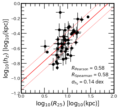
Figure 19 shows the correlation between and for the single-component disk analysis. The resulting relation between the scale height and (left panel) is:
| (15) |
This relationship could be used to estimate as are widely available for most galaxies (). The disk oblateness as a function of the apparent radius is shown in the right panel of Figure 19 with weak correlation coefficients of and as well as a p-value of 0.47. We also report a correlation between and but also between and (Figure 20). While the correlations are comparable with the one obtained from single-component , the relation obtained from the thick disk is slightly weaker and the one from the thin disk is significantly better (for the thick disk dex and for the thin disk dex). This could be due to the fact that both the thin disk and are at the edge of star-forming regions. The best-fit linear models are:
| (16) | ||||
| (17) |


3.4.3 Scale height and


In the left panel Figure 21, we show the correlation between the thin disk scale heights and the maximum velocity retrieved from HyperLEDA. This figure shows that the scale heights increase with , although the scatter tends to be greater for lower maximum velocity km s-1. The correlation have a Pearson correlation coefficient of 0.42, a Spearman coefficient of 0.31 and a p-value of 0.03 with an overall scatter of 0.19 dex. This trend is consistent with the previous findings of YD6 and Comerón et al. (2011b). However, a majority of our scale heights are consistently lower than the ones from YD6. Nonetheless, our uncorrected-for-inclination values are relatively closer to their (right panel) an observation that is previously discussed in Section 3.2. We report a weak correlation between the uncorrected thin disk scale heights and ( dex. Galaxies with bad thick disk results (considered to be without thick disk) are observed to have . This agrees with the observations of Comerón et al. (2018) who found that all the 17 galaxies without a thick disk in their sample of 141 galaxies have a circular velocity below accounting for the gas and a possible third stellar component. However, we also find a moderate anti-correlation between the scale height ratio and the maximum velocity (Figure 22) with that shows that thick disks are more prominent in lower mass, two-component disk galaxies.
The corresponding relations are:
| (18) | ||||
| (19) |
3.4.4 Scale height and other global and photometric properties
Left panel of Figure 23 shows the one-component scale height from Galfit as a function of the central surface brightness . We report a weak correlation with correlation coefficients of and , a p-value of 0.37 and a scatter dex. For consistency with previous studies, we also test our radial-to-vertical scale length ratio against . In the right panel of Figure 23, we present the correlation we find along with scaling relation obtained by Zasov & Bizyaev (2003) using R- and K- band data. Both their samples (square symbols indicating R-band data points and triangles representing K-band elements) returned good correlations, however, our data shows no such correlation (back full circles) yielding a weak interdependence (, , , dex). The reason why the correlation is weak in the 3.6 m-band is unclear. However, unlike our direct model-fitting methods, they estimated the scale height from the scale length and using the observed axis ratio. Additionally, if such a relation exists, it is likely wavelength-dependent as the correlation from Zasov & Bizyaev (2003) seem to be different in the R- and K- band.


We also tested our scale height results as well as ratio against the total stellar mass and the morphological type T (both values were issued from the S4G archive). However, the relations that we find have and thus have been rejected.
3.4.5 Correlation comparison
To probe the a fundamental relation amongst the different correlations, we perform partial correlations for single and two-component scale heights as presented in Figure 24. We observe that the most intrinsic correlation is the relationship. The correlation between the scale height and apparent radius is the second-best relationship that we found. However, Figure 24 shows that this correlation stems from a more intrinsic relation with . The relation is the third-most intrinsic correlation we found. This relationship is dependent on and as observed in the figure. This is reasonable due to the existence of the intrinsic correlation as well as the size-velocity relation (e.g. Mo et al. 1998; McGaugh 2021).


4 Summary
We have measured the stellar disk thickness of 46 edge-on galaxies selected from the Spitzer Survey of Stellar Structure in Galaxies S4G survey by fitting the vertical profile using simple models. Near-infrared images are known to trace the bulk of the stellar mass and are less affected by dust obstruction. The effect of inclination is carefully corrected in all measurements using synthetic images from the GALMER simulations. We use 1D, 2D, and 3D techniques to measure the disk thickness and coherently compare the performance of these three methods. Our findings are the following:
-
•
After comparing the uncertainties of the results from the different methods, we found that the 3D Imfit and 2D Galfit EdgeOnDisk models have the lowest uncertainties. The single disk component fits showed that our inclination correction 1D measurements were consistent with 3D models.
-
•
Our two-component fits reveal that about two-thirds of our sample showed evidence of a thick disk. Yet, none of our galaxies have the traditional thick disk scale height of . This could be the effect of our sample size or the wavelength band that is used. Most of the disks are also vertically symmetrical. We also find that thick disks are 2.65 times larger than thin disks on average. Our analyses on the scale height at specific radii of galaxy disks also prove the existence of disk flaring which is consistent with previous studies. The flaring amplitude is more significant for early-type spirals.
-
•
We also found correlations between the vertical scale height with other galaxy properties as follows:
-
1.
The single-component scale height grows with increasing scale length. However, the radial-to-vertical scale length ratio seems to be constant.
-
2.
Scale heights from both one and two-component models rise with apparent radius .
-
3.
One-component and thin disk tend to increase with the maximum velocity.
-
1.
After performing partial correlation tests, we find that the relation between the scale height and scale length is an intrinsic relationship. This relation could be used for single-component scale height estimations. The relation between scale height and can also be used for two-component thickness estimation.
Acknowledgements
NR acknowledges financial support from the IAU GA, Astronomy in Africa Scholarship. KMD and TSG thanks the support of the Serrapilheira Institute (grant Serra-1709-17357) as well as that of the Brazilian National Research Council (CNPq 308584/2022-8) and of the Rio de Janeiro Research Foundation (FAPARJ grant E-32/200.952/2022), Brazil. The financial assistance of the South African Radio Astronomy Observatory (SARAO) towards this research is hereby acknowledged (www.sarao.ac.za).
Data Availability
The data used in this work are publicly available as part of the S4G project (https://irsa.ipac.caltech.edu/data/SPITZER/S4G/). Derived properties and the scripts used for the analysis will be made available upon reasonable request to the author.
References
- Alard (2000) Alard, C. 2000, arXiv e-prints, astro, doi: 10.48550/arXiv.astro-ph/0007013
- Aoki et al. (1991) Aoki, T. E., Hiromoto, N., Takami, H., & Okamura, S. 1991, PASJ, 43, 755
- Astropy Collaboration et al. (2013) Astropy Collaboration, Robitaille, T. P., Tollerud, E. J., et al. 2013, A&A, 558, A33, doi: 10.1051/0004-6361/201322068
- Astropy Collaboration et al. (2018) Astropy Collaboration, Price-Whelan, A. M., Sipőcz, B. M., et al. 2018, AJ, 156, 123, doi: 10.3847/1538-3881/aabc4f
- Bacchini et al. (2019) Bacchini, C., Fraternali, F., Iorio, G., & Pezzulli, G. 2019, A&A, 622, A64, doi: 10.1051/0004-6361/201834382
- Banerjee & Jog (2007) Banerjee, A., & Jog, C. J. 2007, ApJ, 662, 335, doi: 10.1086/517605
- Bershady et al. (2010) Bershady, M. A., Verheijen, M. A. W., Westfall, K. B., et al. 2010, ApJ, 716, 234, doi: 10.1088/0004-637X/716/1/234
- Bizyaev & Mitronova (2002) Bizyaev, D., & Mitronova, S. 2002, A&A, 389, 795, doi: 10.1051/0004-6361:20020633
- Bizyaev & Mitronova (2009) —. 2009, ApJ, 702, 1567, doi: 10.1088/0004-637X/702/2/1567
- Bradley et al. (2020) Bradley, L., Sipőcz, B., Robitaille, T., et al. 2020, astropy/photutils: 1.0.0, 1.0.0, Zenodo, doi: 10.5281/zenodo.4044744
- Casasola et al. (2017) Casasola, V., Cassarà, L. P., Bianchi, S., et al. 2017, A&A, 605, A18, doi: 10.1051/0004-6361/201731020
- Chilingarian et al. (2010) Chilingarian, I. V., Di Matteo, P., Combes, F., Melchior, A. L., & Semelin, B. 2010, A&A, 518, A61, doi: 10.1051/0004-6361/200912938
- Comerón et al. (2018) Comerón, S., Salo, H., & Knapen, J. H. 2018, A&A, 610, A5, doi: 10.1051/0004-6361/201731415
- Comerón et al. (2011a) Comerón, S., Knapen, J. H., Sheth, K., et al. 2011a, ApJ, 729, 18, doi: 10.1088/0004-637X/729/1/18
- Comerón et al. (2011b) Comerón, S., Elmegreen, B. G., Knapen, J. H., et al. 2011b, ApJ, 741, 28, doi: 10.1088/0004-637X/741/1/28
- de Grijs & van der Kruit (1996) de Grijs, R., & van der Kruit, P. C. 1996, A&AS, 117, 19
- de Jong (1996) de Jong, R. S. 1996, A&AS, 118, 557. https://arxiv.org/abs/astro-ph/9601002
- Dubois et al. (2021) Dubois, Y., Beckmann, R., Bournaud, F., et al. 2021, A&A, 651, A109, doi: 10.1051/0004-6361/202039429
- Erwin (2015) Erwin, P. 2015, ApJ, 799, 226, doi: 10.1088/0004-637X/799/2/226
- Eskew et al. (2012) Eskew, M., Zaritsky, D., & Meidt, S. 2012, AJ, 143, 139, doi: 10.1088/0004-6256/143/6/139
- Evans et al. (1998) Evans, N. W., Gyuk, G., Turner, M. S., & Binney, J. 1998, ApJ, 501, L45, doi: 10.1086/311451
- Fazio et al. (2004) Fazio, G. G., Hora, J. L., Allen, L. E., et al. 2004, ApJS, 154, 10, doi: 10.1086/422843
- Freeman (1970) Freeman, K. C. 1970, ApJ, 160, 811, doi: 10.1086/150474
- Haslbauer et al. (2022) Haslbauer, M., Banik, I., Kroupa, P., Wittenburg, N., & Javanmardi, B. 2022, ApJ, 925, 183, doi: 10.3847/1538-4357/ac46ac
- Helmi et al. (2018) Helmi, A., Babusiaux, C., Koppelman, H. H., et al. 2018, Nature, 563, 85, doi: 10.1038/s41586-018-0625-x
- Hopkins et al. (2018) Hopkins, P. F., Wetzel, A., Kereš, D., et al. 2018, MNRAS, 480, 800, doi: 10.1093/mnras/sty1690
- Kasparova et al. (2016) Kasparova, A. V., Katkov, I. Y., Chilingarian, I. V., et al. 2016, MNRAS, 460, L89, doi: 10.1093/mnrasl/slw083
- Kregel et al. (2005) Kregel, M., van der Kruit, P. C., & Freeman, K. C. 2005, MNRAS, 358, 503, doi: 10.1111/j.1365-2966.2005.08855.x
- Lange et al. (2016) Lange, R., Moffett, A. J., Driver, S. P., et al. 2016, MNRAS, 462, 1470, doi: 10.1093/mnras/stw1495
- Larsen & Humphreys (2003) Larsen, J. A., & Humphreys, R. M. 2003, AJ, 125, 1958, doi: 10.1086/368364
- Lee et al. (1993) Lee, M. G., Freedman, W. L., & Madore, B. F. 1993, ApJ, 417, 553, doi: 10.1086/173334
- Makarov et al. (2014) Makarov, D., Prugniel, P., Terekhova, N., Courtois, H., & Vauglin, I. 2014, A&A, 570, A13, doi: 10.1051/0004-6361/201423496
- McGaugh (2021) McGaugh, S. S. 2021, Studies in History and Philosophy of Science, 88, 220, doi: 10.1016/j.shpsa.2021.05.008
- Mo et al. (1998) Mo, H. J., Mao, S., & White, S. D. M. 1998, MNRAS, 295, 319, doi: 10.1046/j.1365-8711.1998.01227.x
- Müller et al. (2017) Müller, P., Krause, M., Beck, R., & Schmidt, P. 2017, A&A, 606, A41, doi: 10.1051/0004-6361/201731257
- Newville et al. (2016) Newville, M., Stensitzki, T., Allen, D. B., et al. 2016, Lmfit: Non-Linear Least-Square Minimization and Curve-Fitting for Python. http://ascl.net/1606.014
- O’Brien et al. (2010) O’Brien, J. C., Freeman, K. C., & van der Kruit, P. C. 2010, A&A, 515, A63, doi: 10.1051/0004-6361/200912568
- Oh et al. (2008) Oh, S.-H., de Blok, W. J. G., Walter, F., Brinks, E., & Kennicutt, Robert C., J. 2008, AJ, 136, 2761, doi: 10.1088/0004-6256/136/6/2761
- Peng et al. (2010) Peng, C. Y., Ho, L. C., Impey, C. D., & Rix, H.-W. 2010, AJ, 139, 2097, doi: 10.1088/0004-6256/139/6/2097
- Qu et al. (2011) Qu, Y., Di Matteo, P., Lehnert, M. D., & van Driel, W. 2011, A&A, 530, A10, doi: 10.1051/0004-6361/201015224
- Querejeta et al. (2015) Querejeta, M., Meidt, S. E., Schinnerer, E., et al. 2015, ApJS, 219, 5, doi: 10.1088/0067-0049/219/1/5
- Reid & Majewski (1993) Reid, N., & Majewski, S. R. 1993, ApJ, 409, 635, doi: 10.1086/172695
- Sarkar & Jog (2019) Sarkar, S., & Jog, C. J. 2019, A&A, 628, A58, doi: 10.1051/0004-6361/201935430
- Schwarzkopf & Dettmar (2000) Schwarzkopf, U., & Dettmar, R. J. 2000, A&A, 361, 451. https://arxiv.org/abs/astro-ph/0007104
- Seth et al. (2005) Seth, A. C., Dalcanton, J. J., & de Jong, R. S. 2005, AJ, 130, 1574, doi: 10.1086/444620
- Sheth et al. (2010) Sheth, K., Regan, M., Hinz, J. L., et al. 2010, PASP, 122, 1397, doi: 10.1086/657638
- Sotillo-Ramos et al. (2023) Sotillo-Ramos, D., Donnari, M., Pillepich, A., et al. 2023, MNRAS, 523, 3915, doi: 10.1093/mnras/stad1485
- Ting & Rix (2019) Ting, Y.-S., & Rix, H.-W. 2019, ApJ, 878, 21, doi: 10.3847/1538-4357/ab1ea5
- van der Kruit (1988) van der Kruit, P. C. 1988, A&A, 192, 117
- van der Kruit & Searle (1981) van der Kruit, P. C., & Searle, L. 1981, A&A, 95, 105
- Vieira et al. (2022) Vieira, K., Carraro, G., Korchagin, V., et al. 2022, ApJ, 932, 28, doi: 10.3847/1538-4357/ac6b9b
- Xilouris et al. (1999) Xilouris, E. M., Byun, Y. I., Kylafis, N. D., Paleologou, E. V., & Papamastorakis, J. 1999, A&A, 344, 868. https://arxiv.org/abs/astro-ph/9901158
- Xilouris et al. (1997) Xilouris, E. M., Kylafis, N. D., Papamastorakis, J., Paleologou, E. V., & Haerendel, G. 1997, A&A, 325, 135
- Yi et al. (2023) Yi, S. K., Jang, J. K., Devriendt, J., et al. 2023, arXiv e-prints, arXiv:2308.03566, doi: 10.48550/arXiv.2308.03566
- Yoachim & Dalcanton (2006) Yoachim, P., & Dalcanton, J. J. 2006, AJ, 131, 226, doi: 10.1086/497970
- Yu et al. (2023) Yu, S., Bullock, J. S., Gurvich, A. B., et al. 2023, MNRAS, 523, 6220, doi: 10.1093/mnras/stad1806
- Yuan & Zhu (2004) Yuan, Q.-r., & Zhu, C.-x. 2004, Chinese Astron. Astrophys., 28, 127, doi: 10.1016/S0275-1062(04)90015-X
- Zasov & Bizyaev (2003) Zasov, A. V., & Bizyaev, D. V. 2003, in EAS Publications Series, Vol. 10, EAS Publications Series, ed. C. M. Boily, P. Patsis, S. Portegies Zwart, R. Spurzem, & C. Theis, 121. https://arxiv.org/abs/astro-ph/0212333