This paper was converted on www.awesomepapers.org from LaTeX by an anonymous user.
Want to know more? Visit the Converter page.

On the solution of the coupled steady-state dual-porosity-Navier-Stokes fluid flow model with the Beavers-Joseph-Saffman interface condition11footnotemark: 1

Di Yang [email protected] Yinnian He [email protected] Luling Cao [email protected] School of Mathematics and Statistics, Xi’an Jiaotong University, Xi’an, Shaanxi 710049, P.R. China
Abstract

In this work, we propose a new analysis strategy to establish an a priori estimate of the weak solutions to the coupled steady-state dual-porosity-Navier-Stokes fluid flow model with the Beavers-Joseph-Saffman interface condition. The most advantage of our proposed method is that the a priori estimate and the existence result are independent of small data and the large viscosity restriction. Therefore the global uniqueness of the weak solution is naturally obtained.

keywords:
weak solution, dual-porosity-Navier-Stokes, Beavers-Joseph-Saffman interface condition, a priori estimate, existence, global uniqueness
journal:

1 Introduction

Coupled free flow and porous medium flow systems play an important role in many practical engineering fields, e.g., the flood simulation of arid areas in geological science [20], filtration treatment in industrial production [28, 37], petroleum exploitation in mining, and blood penetration between vessels and organs in life science [19]. Specifically, the systems are usually described by Navier-Stokes equations (or Stokes equations) coupled with Darcy’s equation, and there are amounts of achievements such as [12, 13, 10, 16, 26, 36, 48]. However, the standard Darcy’s equation describes fluids flowing through only a single porosity medium, which is not accurate to deal with the complicated multiple porous media similar to naturally fractured reservoir. Actually, the naturally fractured reservoir is comprised of low permeable rock matrix blocks surrounded by an irregular network of natural microfractures, and further they have different fluid storage and conductivity properties [43, 47]. In 2016, Hou et al. [31] proposed and numerically solved a coupled dual-porosity-Stokes fluid flow model with four multi-physics interface conditions. The authors used the dual-porosity equations over Darcy’s region to describe fluid flowing through the multiple porous medium. Recently, several related research on the above model can be found in the literatures [2, 3, 24, 29, 44]. In particular, Gao and Li [24] proposed a decoupled stabilized finite element method to solve the coupled dual-porosity-Navier-Stokes fluid flow model in the numerical field.

The steady-state dual-porosity-Navier-Stokes fluid flow model has distinct features and difficulties in mathematical analysis. Many numerical methods have been studied for the well-known stationary or time-dependent Navier-Stokes/Darcy model with Beavers-Joseph or Beaver-Joseph-Saffman interface condition, including coupled finite element methods [6, 11, 21, 22, 49], discontinuous Galerkin methods [17, 26, 27], domain decomposition methods [12, 20, 21, 30, 38], and decoupled methods based on two-grid finite element [10, 23, 48, 49]. In spite of the above great contributions to numerical simulation, the existence of a weak solution to the coupled dual-porosity-Navier-Stokes fluid flow model with Beavers-Joseph-Saffman interface condition for general data keeps unresolved. In many literatures [6, 10, 17, 20, 21, 22, 26, 27, 30, 49], a priori estimates and existence of a weak solution need suitable small data and/or large viscosity restrictions, and therefore only local uniqueness can be established when the data satisfy additional restrictions. In [26], the authors pointed out that the difficulty for a priori estimates and existence with general data is stemmed from the transmission interface condition, which does not completely compensate the nonlinear convection term from the Navier-Stokes equations in the energy balance.

Therefore in this paper, stemming from resolving steady-state Navier-Stokes equations with mixed boundary conditions in [32], we shall establish a new a priori estimate of the weak solutions by coupling the model problem with a designed auxiliary problem in order to completely compensate the nonlinear convection term from the Navier-Stokes equations. In addition, we shall also prove existence of a weak solution without small data or large viscosity restriction. As a result, the global uniqueness of the weak solution is naturally obtained.

The rest of this paper is organized as follows. In Section 2, we specify the steady-state dual-porosity-Navier-Stokes fluid flow model with Beavers-Joseph-Saffman interface condition and provide its Galerkin variational formulation. In Section 3, we establish a new a priori estimate of the weak solutions by coupling the model problem with an auxiliary problem, which is designed subject to the model problem. Finally, in Section 4, we prove existence of the weak solution without small data and/or large viscosity restriction by the Galerkin method and Brouwer’s fixed-point theorem, and global uniqueness of all variables by the inf-sup condition and Babus̆ka–Brezzi’s theory.

2 Model specification

2.1 Setting of the problem

In this section, we consider the steady-state dual-porosity-Navier-Stokes fluid flow model in a bounded open polygonal domain ΩN(N=2,3)\Omega\subset\mathbb{R}^{N}(N=2,3) with four physically valid interface conditions.
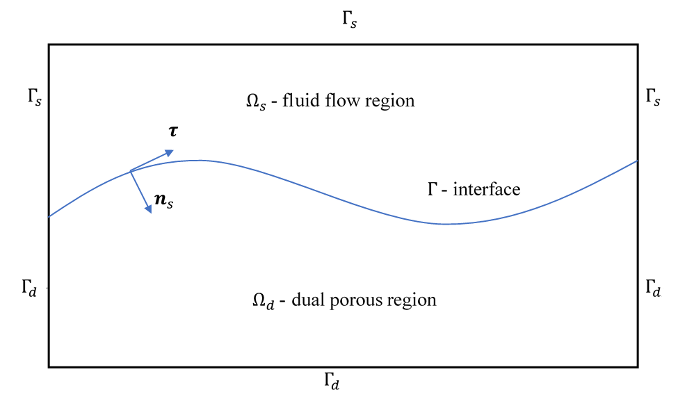
Refer to caption
Figure 1: Schematic representation of fluid flow region Ωs\Omega_{s} and dual-porous medium region Ωd\Omega_{d}, separated by an interface Γ\Gamma.

The domain Ω\Omega consists of a fluid flow region Ωs\Omega_{s} and a dual-porous medium region Ωd\Omega_{d}, with interface Γ=Ω¯sΩ¯d\Gamma=\overline{\Omega}_{s}\cap\overline{\Omega}_{d} (see Figure 1). Both Ωs\Omega_{s} and Ωd\Omega_{d} are open, regular, simply connected, and bounded with Lipschitz continuous boundaries Γi=ΩiΓ(i=s,d)\Gamma_{i}=\partial\Omega_{i}\setminus\Gamma~{}(i=s,d), respectively. Here, ΩsΩd=\Omega_{s}\cap\Omega_{d}=\emptyset, Ω¯sΩ¯d=Ω\overline{\Omega}_{s}\cup\overline{\Omega}_{d}=\Omega. The unit normal vector of the interface Γ\Gamma pointing from Ωs\Omega_{s} to Ωd\Omega_{d} (from Ωd\Omega_{d} to Ωs\Omega_{s}) is denoted by 𝒏s\bm{n}_{s} (resp. 𝒏d\bm{n}_{d}), and the corresponding unit tangential vectors are denoted by 𝝉i\bm{\tau}_{i}, i=1,,N1i=1,\cdots,N-1. In two-dimensional case, if we write 𝒏s=(n1,n2)2\bm{n}_{s}=(n_{1},n_{2})\in\mathbb{R}^{2}, then 𝝉=𝒏s=(n2,n1)\bm{\tau}=\bm{n}_{s}^{\top}=(-n_{2},n_{1}).

In Ωs\Omega_{s}, the fluid flow is governed by the Navier-Stokes equation [11, 12, 17, 20, 21, 26, 27]:

{(𝒖s)𝒖s𝕋(𝒖s,ps)=𝒇sinΩs,𝒖s=0inΩs,𝒖s=𝟎onΓs,\begin{cases}\left(\bm{u}_{s}\cdot\nabla\right)\bm{u}_{s}-\nabla\cdot\mathbb{T}(\bm{u}_{s},p_{s})=\bm{f}_{s}&\text{in}~{}\Omega_{s},\\ \nabla\cdot\bm{u}_{s}=0&\text{in}~{}\Omega_{s},\\ \bm{u}_{s}=\bm{0}&\text{on}~{}\Gamma_{s},\end{cases} (2.1)

where 𝕋(𝒖s,ps)=ps𝕀+2ν𝔻(𝒖s)\mathbb{T}(\bm{u}_{s},p_{s})=-p_{s}\mathbb{I}+2\nu\mathbb{D}(\bm{u}_{s}) is the stress tensor, ν\nu is the kinetic viscosity, 𝔻(𝒖s)=12[𝒖s+(𝒖s)]\mathbb{D}(\bm{u}_{s})=\frac{1}{2}\left[\nabla\bm{u}_{s}+(\nabla\bm{u}_{s})^{\top}\right] is the velocity deformation tensor, 𝒖s(𝒙)\bm{u}_{s}(\bm{x}) denotes the fluid velocity in Ωs\Omega_{s}, ps(𝒙)p_{s}(\bm{x}) denotes the kinematic pressure in Ωs\Omega_{s}, and 𝒇s(𝒙)\bm{f}_{s}(\bm{x}) denotes a general body force term that includes gravitational acceleration. As usual, we write formally:

(𝒗)𝒘=i=1Nvi𝒘xi,𝒗=i=1Nvixi.(\bm{v}\cdot\nabla)\bm{w}=\sum_{i=1}^{N}v_{i}\frac{\partial\bm{w}}{\partial x_{i}},\quad\nabla\cdot\bm{v}=\sum_{i=1}^{N}\frac{\partial v_{i}}{\partial x_{i}}.

The filtration of an incompressible fluid through porous media is often described using Darcy’s law. So in dual-porous medium domain Ωd\Omega_{d}, the flow is governed by a traditional dual-porosity model, which is composed of matrix and microfracture equations as follows:

{(kmμϕm)+σkmμ(ϕmϕf)=0inΩd,(kfμϕf)+σkmμ(ϕfϕm)=fdinΩd,ϕm=0onΓd,ϕf=0onΓd,\begin{cases}-\nabla\cdot\big{(}\frac{k_{m}}{\mu}\nabla\phi_{m}\big{)}+\frac{\sigma k_{m}}{\mu}(\phi_{m}-\phi_{f})=0&\text{in}~{}\Omega_{d},\\ -\nabla\cdot\big{(}\frac{k_{f}}{\mu}\nabla\phi_{f}\big{)}+\frac{\sigma k_{m}}{\mu}(\phi_{f}-\phi_{m})=f_{d}&\text{in}~{}\Omega_{d},\\ \phi_{m}=0&\text{on}~{}\Gamma_{d},\\ \phi_{f}=0&\text{on}~{}\Gamma_{d},\end{cases} (2.2)

where ϕm(𝒙)\phi_{m}(\bm{x}), ϕf(𝒙)\phi_{f}(\bm{x}) denote the matrix and microfracture flow pressure, μ\mu is the dynamic viscosity, kmk_{m}, kfk_{f} are the intrinsic permeability of the matrix and microfracture regions, σ\sigma is the shape factor characterizing the morphology and dimension of the microfractures, fdf_{d} is the sink/source term for the microfractures, and the term σkmμ(ϕmϕf)\frac{\sigma k_{m}}{\mu}(\phi_{m}-\phi_{f}) describes the mass exchange between matrix and microfractures.

Based on the fundamental properties of the dual-porosity fluid flow model and traditional Stokes–Darcy flow model, Hou et al. [31] introduced four physically valid interface conditions as follows to couple appropriately the dual-porosity-Stokes model, which are also adapted to our problem.

  • 1.

    No-exchange condition between the matrix and the conduits/macrofractures:

    kmμϕm𝒏d=0onΓ.-\frac{k_{m}}{\mu}\nabla\phi_{m}\cdot\bm{n}_{d}=0\quad\text{on}~{}\Gamma. (2.3)
  • 2.

    Mass conservation:

    𝒖s𝒏s=kfμϕf𝒏donΓ.\bm{u}_{s}\cdot\bm{n}_{s}=\frac{k_{f}}{\mu}\nabla\phi_{f}\cdot\bm{n}_{d}\quad\text{on}~{}\Gamma. (2.4)
  • 3.

    Balance of normal forces:

    𝒏s(𝕋(𝒖s,ps)𝒏s)=ϕfρonΓ.-\bm{n}_{s}\cdot(\mathbb{T}(\bm{u}_{s},p_{s})\bm{n}_{s})=\frac{\phi_{f}}{\rho}\quad\text{on}~{}\Gamma. (2.5)
  • 4.

    The Beavers-Joseph-Saffman interface condition [7, 33, 35, 41]: for i=1,,N1i=1,\cdots,N-1,

    𝝉i(𝕋(𝒖s,ps)𝒏s)=ανNtrace(𝚷)𝒖s𝝉ionΓ.-\bm{\tau}_{i}\cdot\left(\mathbb{T}(\bm{u}_{s},p_{s})\bm{n}_{s}\right)=\frac{\alpha\nu\sqrt{N}}{\sqrt{\text{trace}(\bm{\Pi})}}\bm{u}_{s}\cdot\bm{\tau}_{i}\quad\text{on}~{}\Gamma. (2.6)

In (2.3)–(2.6), α\alpha is the Beavers-Joseph constant depending on the properties of the dual-porous medium, 𝚷\bm{\Pi} represents the intrinsic permeability that satisfies the relation 𝚷=kf𝕀\bm{\Pi}=k_{f}\mathbb{I}, 𝕀\mathbb{I} is the N×NN\times N identity matrix, and ρ\rho is the fluid density.

2.2 Galerkin variational formulation

Throughout this paper we use the following standard function spaces. For a Lipschitz domain 𝒟N\mathcal{D}\subset\mathbb{R}^{N}, N1N\geqslant 1, we denote by Wk,p(𝒟)W^{k,p}(\mathcal{D}) the Sobolev space with indexes k0k\geqslant 0, 1p1\leqslant p\leqslant\infty of real-valued functions defined on 𝒟\mathcal{D}, endowed with the seminorm ||Wk,p(𝒟)|\cdot|_{W^{k,p}(\mathcal{D})} denoted by ||k,p,𝒟|\cdot|_{k,p,\mathcal{D}} and norm Wk,p(𝒟)\|\cdot\|_{W^{k,p}(\mathcal{D})} denoted by k,p,𝒟\|\cdot\|_{k,p,\mathcal{D}} [1]. When p=2p=2, Ws,2(𝒟)W^{s,2}(\mathcal{D}) is denoted as Hk(𝒟)H^{k}(\mathcal{D}) and the corresponding seminorm and norm are written as ||k,𝒟|\cdot|_{k,\mathcal{D}} and k,𝒟\|\cdot\|_{k,\mathcal{D}}, respectively. In addition, with |𝒟||\mathcal{D}| we denote the NN-dimensional Hausdorff measure of 𝒟\mathcal{D}.

To perform the variational formulation, we define some necessary Hilbert spaces given by

𝑿s\displaystyle\bm{X}_{s} :={𝒗𝑯1(Ωs):𝒗=𝟎onΓs},\displaystyle:=\left\{\bm{v}\in\bm{H}^{1}(\Omega_{s}):\bm{v}=\bm{0}~{}\text{on}~{}\Gamma_{s}\right\},
Xd\displaystyle X_{d} :={ψH1(Ωd):ψ=0onΓd},\displaystyle:=\left\{\psi\in H^{1}(\Omega_{d}):\psi=0~{}\text{on}~{}\Gamma_{d}\right\},
Qs\displaystyle Q_{s} :=L2(Ωs).\displaystyle:=L^{2}(\Omega_{s}).

We also need the trace space 𝑯001/2(Γ):=𝑿s|Γ\bm{H}_{00}^{1/2}(\Gamma):=\bm{X}_{s}|_{\Gamma} (resp. H001/2(Γ):=Xd|ΓH_{00}^{1/2}(\Gamma):=X_{d}|_{\Gamma}), which is a nonclosed subspace of 𝑯1/2(Γ)\bm{H}^{1/2}(\Gamma) (resp. H1/2(Γ)H^{1/2}(\Gamma)) and has a continuous zero extension to 𝑯1/2(Ωs)\bm{H}^{1/2}(\partial\Omega_{s}) (resp. H1/2(Ωd)H^{1/2}(\partial\Omega_{d})) [14, 15, 20]. For the trace space 𝑯001/2(Γ)\bm{H}_{00}^{1/2}(\Gamma) and its dual space (𝑯001/2(Γ))(\bm{H}_{00}^{1/2}(\Gamma))^{\prime}, we have the following continuous imbedding result [15]:

𝑯001/2(Γ)𝑯1/2(Γ)𝑳2(Γ)𝑯1/2(Γ)(𝑯001/2(Γ)).\bm{H}_{00}^{1/2}(\Gamma)\subsetneqq\bm{H}^{1/2}(\Gamma)\subsetneqq\bm{L}^{2}(\Gamma)\subsetneqq\bm{H}^{-1/2}(\Gamma)\subsetneqq(\bm{H}_{00}^{1/2}(\Gamma))^{\prime}. (2.7)

One can see more details in [15, 34, 45] and the references therein. For any bounded domain 𝒟N\mathcal{D}\subset\mathbb{R}^{N}, (,)𝒟(\cdot,\cdot)_{\mathcal{D}} denotes the L2L^{2} inner product on 𝒟\mathcal{D}, and ,𝒟\langle\cdot,\cdot\rangle_{\partial\mathcal{D}} denotes the L2L^{2} inner product (or duality pairing) on the boundary 𝒟\partial\mathcal{D}. We also consider the following product Hilbert space 𝒀¯:=𝑿s×Xd×Xd\underline{\bm{Y}}:=\bm{X}_{s}\times X_{d}\times X_{d} with norm

𝒘¯𝒀¯=(𝒘s1,Ωs2+ψm1,Ωd2+ψf1,Ωd2)1/2,𝒘¯=(𝒘s,ψm,ψf)𝒀¯.\|\underline{\bm{w}}\|_{\underline{\bm{Y}}}=\Big{(}\|\bm{w}_{s}\|_{1,\Omega_{s}}^{2}+\|\psi_{m}\|_{1,\Omega_{d}}^{2}+\|\psi_{f}\|_{1,\Omega_{d}}^{2}\Big{)}^{1/2},\quad\forall\,\underline{\bm{w}}=(\bm{w}_{s},\psi_{m},\psi_{f})\in\underline{\bm{Y}}.

In addition, based on the following formula:

((𝒖)𝒗,𝒘)𝒟=𝒖𝒏,𝒗𝒘𝒟((𝒖)𝒘,𝒗)𝒟((𝒖)𝒗,𝒘)𝒟,𝒖,𝒗,𝒘𝑯1(𝒟),\left((\bm{u}\cdot\nabla)\bm{v},\bm{w}\right)_{\mathcal{D}}=\left\langle\bm{u}\cdot\bm{n},\bm{v}\cdot\bm{w}\right\rangle_{\partial\mathcal{D}}-\left((\bm{u}\cdot\nabla)\bm{w},\bm{v}\right)_{\mathcal{D}}-\left((\nabla\cdot\bm{u})\bm{v},\bm{w}\right)_{\mathcal{D}},\quad\forall\,\bm{u},\bm{v},\bm{w}\in\bm{H}^{1}(\mathcal{D}),

we introduce the trilinear form b(;,)b(\cdot;\cdot,\cdot) given by 𝒖s,𝒗s,𝒘s𝑿s\forall\,\bm{u}_{s},\bm{v}_{s},\bm{w}_{s}\in\bm{X}_{s},

b(𝒖s;𝒗s,𝒘s)=((𝒖s)𝒗s,𝒘s)Ωs+12((𝒖s)𝒗s,𝒘s)Ωs=12𝒖s𝒏s,𝒗s𝒘sΓ+12((𝒖s)𝒗s,𝒘s)Ωs12((𝒖s)𝒘s,𝒗s)Ωs.\begin{split}b(\bm{u}_{s};\bm{v}_{s},\bm{w}_{s})&=\left((\bm{u}_{s}\cdot\nabla)\bm{v}_{s},\bm{w}_{s}\right)_{\Omega_{s}}+\frac{1}{2}\left((\nabla\cdot\bm{u}_{s})\bm{v}_{s},\bm{w}_{s}\right)_{\Omega_{s}}\\ &=\frac{1}{2}\left\langle\bm{u}_{s}\cdot\bm{n}_{s},\bm{v}_{s}\cdot\bm{w}_{s}\right\rangle_{\Gamma}+\frac{1}{2}\left((\bm{u}_{s}\cdot\nabla)\bm{v}_{s},\bm{w}_{s}\right)_{\Omega_{s}}-\frac{1}{2}\left((\bm{u}_{s}\cdot\nabla)\bm{w}_{s},\bm{v}_{s}\right)_{\Omega_{s}}.\end{split} (2.8)

Hence, the Galerkin variational formulation of the coupled problem (2.1)–(2.6) is proposed that: to find (𝒖¯,ps)𝒀¯×Qs(\underline{\bm{u}},p_{s})\in\underline{\bm{Y}}\times Q_{s} such that

a(𝒖¯,𝒗¯)+d(𝒗s,ps)d(𝒖s,qs)+b(𝒖s;𝒖s,𝒗s)=ρ(𝒇s,𝒗s)Ωs+(fd,ψf)Ωd,(𝒗¯,qs)𝒀¯×Qs,a(\underline{\bm{u}},\underline{\bm{v}})+d(\bm{v}_{s},p_{s})-d(\bm{u}_{s},q_{s})+b(\bm{u}_{s};\bm{u}_{s},\bm{v}_{s})=\rho(\bm{f}_{s},\bm{v}_{s})_{\Omega_{s}}+(f_{d},\psi_{f})_{\Omega_{d}},\quad\forall\,(\underline{\bm{v}},q_{s})\in\underline{\bm{Y}}\times Q_{s}, (2.9)

where 𝒖¯=(𝒖s,ϕm,ϕf)\underline{\bm{u}}=(\bm{u}_{s},\phi_{m},\phi_{f}), 𝒗¯=(𝒗s,ψm,ψf)\underline{\bm{v}}=(\bm{v}_{s},\psi_{m},\psi_{f}), the bilinear forms a(,)a(\cdot,\cdot) and d(,)d(\cdot,\cdot) are defined as

as(𝒖¯,𝒗¯)\displaystyle a_{s}(\underline{\bm{u}},\underline{\bm{v}}) =2ρν(𝔻(𝒖s),𝔻(𝒗s))Ωs,\displaystyle=2\rho\nu\left(\mathbb{D}(\bm{u}_{s}),\mathbb{D}(\bm{v}_{s})\right)_{\Omega_{s}},
ad(𝒖¯,𝒗¯)\displaystyle a_{d}(\underline{\bm{u}},\underline{\bm{v}}) =kmμ(ϕm,ψm)Ωd+kfμ(ϕf,ψf)Ωd+σkmμ(ϕmϕf,ψm)Ωd+σkmμ(ϕfϕm,ψf)Ωd,\displaystyle=\frac{k_{m}}{\mu}\left(\nabla\phi_{m},\nabla\psi_{m}\right)_{\Omega_{d}}+\frac{k_{f}}{\mu}\left(\nabla\phi_{f},\nabla\psi_{f}\right)_{\Omega_{d}}+\frac{\sigma k_{m}}{\mu}\left(\phi_{m}-\phi_{f},\psi_{m}\right)_{\Omega_{d}}+\frac{\sigma k_{m}}{\mu}\left(\phi_{f}-\phi_{m},\psi_{f}\right)_{\Omega_{d}},
aΓ(𝒖¯,𝒗¯)\displaystyle a_{\Gamma}(\underline{\bm{u}},\underline{\bm{v}}) =ϕf,𝒗s𝒏sΓψf,𝒖s𝒏sΓ+i=1N1αρνkf𝒖s𝝉i,𝒗s𝝉iΓ,\displaystyle=\left\langle\phi_{f},\bm{v}_{s}\cdot\bm{n}_{s}\right\rangle_{\Gamma}-\left\langle\psi_{f},\bm{u}_{s}\cdot\bm{n}_{s}\right\rangle_{\Gamma}+\sum_{i=1}^{N-1}\frac{\alpha\rho\nu}{\sqrt{k_{f}}}\left\langle\bm{u}_{s}\cdot\bm{\tau}_{i},\bm{v}_{s}\cdot\bm{\tau}_{i}\right\rangle_{\Gamma},
a(𝒖¯,𝒗¯)\displaystyle a(\underline{\bm{u}},\underline{\bm{v}}) =as(𝒖¯,𝒗¯)+ad(𝒖¯,𝒗¯)+aΓ(𝒖¯,𝒗¯),\displaystyle=a_{s}(\underline{\bm{u}},\underline{\bm{v}})+a_{d}(\underline{\bm{u}},\underline{\bm{v}})+a_{\Gamma}(\underline{\bm{u}},\underline{\bm{v}}),
d(𝒗s,qs)\displaystyle d(\bm{v}_{s},q_{s}) =ρ(𝒗s,qs)Ωs.\displaystyle=-\rho(\nabla\cdot\bm{v}_{s},q_{s})_{\Omega_{s}}.
Remark 2.1.

We note that the term 12((𝐮s)𝐯s,𝐰s)Ωs\frac{1}{2}\left((\nabla\cdot\bm{u}_{s})\bm{v}_{s},\bm{w}_{s}\right)_{\Omega_{s}} vanishes in (2.8) if 𝐮s=0\nabla\cdot\bm{u}_{s}=0.

Remark 2.2.

For the sake of clarity, in our analysis we shall adopt homogenous boundary conditions. In addition, for the general Dirichlet boundary conditions:

𝒖|Γs=𝒖dir,ϕm|Γd=ϕmdir,ϕf|Γd=ϕfdir,\bm{u}|_{\Gamma_{s}}=\bm{u}^{\text{dir}},\quad\phi_{m}|_{\Gamma_{d}}=\phi_{m}^{\text{dir}},\quad\phi_{f}|_{\Gamma_{d}}=\phi_{f}^{\text{dir}},

the standard homogenization technique and the lifting operators employed in [20] can be used to obtain an equivalent system with the homogeneous Dirichlet boundary conditions.

Thanks to [17, 26], we have the following important result:

Lemma 2.1.

Assume that 𝐟s𝐋2(Ωs)\bm{f}_{s}\in\bm{L}^{2}(\Omega_{s}) and fdL2(Ωd)f_{d}\in L^{2}(\Omega_{d}). Then if (𝐮s,ϕf,ϕm,ps)𝐗s×Xd×Xd×Qs(\bm{u}_{s},\phi_{f},\phi_{m},p_{s})\in\bm{X}_{s}\times X_{d}\times X_{d}\times Q_{s} satisfies (2.1)–(2.6), it is also a solution to problem (2.9). Conversely, any solution of problem (2.9) satisfies (2.1)–(2.6).

3 An a priori estimate

In this section, we shall propose an a priori estimate for possible solutions of (2.9).

3.1 Some technique inequalities

Firstly, throughout this paper we use CC to denote a generic positive constant independent of discretization parameters, which may take different values in different occasions. Then, based on general Sobolev inequalities, the trace theorem and the Sobolev embedding theorem [1], we have that for any bounded open set 𝒟N\mathcal{D}\subset\mathbb{R}^{N} with Lipschitz continuous boundary 𝒟\partial\mathcal{D} and for all vH1(𝒟)v\in H^{1}(\mathcal{D}),

v0,q,𝒟\displaystyle\|v\|_{0,q,\mathcal{D}} Cv1,𝒟,1q6,\displaystyle\leqslant C\|v\|_{1,\mathcal{D}},\quad 1\leqslant q\leqslant 6, (3.1)
v0,𝒟\displaystyle\|v\|_{0,\partial\mathcal{D}} Cv0,𝒟1/2v1,𝒟1/2Cv1,𝒟,\displaystyle\leqslant C\|v\|_{0,\mathcal{D}}^{1/2}\|v\|_{1,\mathcal{D}}^{1/2}\leqslant C\|v\|_{1,\mathcal{D}}, (3.2)
v0,4,𝒟\displaystyle\|v\|_{0,4,\partial\mathcal{D}} Cv1,𝒟,\displaystyle\leqslant C\|v\|_{1,\mathcal{D}}, (3.3)

which can be also found in [17, 26]. We also need Poincaré inequality and Korn’s inequality [15] that for all 𝒗s𝑿s\bm{v}_{s}\in\bm{X}_{s} and for all ψXd\psi\in X_{d},

𝒗s0,Ωs\displaystyle\|\bm{v}_{s}\|_{0,\Omega_{s}} C|𝒗s|1,Ωs,\displaystyle\leqslant C|\bm{v}_{s}|_{1,\Omega_{s}}, (3.4)
ψ0,Ωd\displaystyle\|\psi\|_{0,\Omega_{d}} C|ψ|1,Ωd,\displaystyle\leqslant C|\psi|_{1,\Omega_{d}}, (3.5)
|𝒗s|1,Ωs\displaystyle|\bm{v}_{s}|_{1,\Omega_{s}} C𝔻(𝒗s)0,Ωs.\displaystyle\leqslant C\|\mathbb{D}(\bm{v}_{s})\|_{0,\Omega_{s}}. (3.6)

Moreover, for the trilinear form b(;,)b(\cdot;\cdot,\cdot), the following lemma holds with the help of [4, 8], (3.1), (3.4) and (3.6).

Lemma 3.1.

For any functions 𝐮s\bm{u}_{s}, 𝐯s\bm{v}_{s}, 𝐰s𝐗s\bm{w}_{s}\in\bm{X}_{s}, we have

|((𝒖s)𝒗s,𝒘s)Ωs|\displaystyle\left|\left((\bm{u}_{s}\cdot\nabla)\bm{v}_{s},\bm{w}_{s}\right)_{\Omega_{s}}\right| C𝒖s0,Ωs1/2𝔻(𝒖s)0,Ωs1/2𝔻(𝒗s)0,Ωs𝔻(𝒘s)0,Ωs,\displaystyle\leqslant C\|\bm{u}_{s}\|_{0,\Omega_{s}}^{1/2}\|\mathbb{D}(\bm{u}_{s})\|_{0,\Omega_{s}}^{1/2}\|\mathbb{D}(\bm{v}_{s})\|_{0,\Omega_{s}}\|\mathbb{D}(\bm{w}_{s})\|_{0,\Omega_{s}}, (3.7)
|((𝒖s)𝒗s,𝒘s)Ωs|\displaystyle\left|\left((\nabla\cdot\bm{u}_{s})\bm{v}_{s},\bm{w}_{s}\right)_{\Omega_{s}}\right| C𝒗s0,Ωs1/2𝔻(𝒗s)0,Ωs1/2𝔻(𝒖s)0,Ωs𝔻(𝒘s)0,Ωs.\displaystyle\leqslant C\|\bm{v}_{s}\|_{0,\Omega_{s}}^{1/2}\|\mathbb{D}(\bm{v}_{s})\|_{0,\Omega_{s}}^{1/2}\|\mathbb{D}(\bm{u}_{s})\|_{0,\Omega_{s}}\|\mathbb{D}(\bm{w}_{s})\|_{0,\Omega_{s}}. (3.8)

Proof 1.

First, let us recall the standard interpolation inequality [4, 8]: for any bounded open set 𝒟N\mathcal{D}\subset\mathbb{R}^{N} with Lipschitz continuous boundary 𝒟\partial\mathcal{D}, 1p<q<1\leqslant p<q<\infty and θ=N(1/p1/q)1\theta=N(1/p-1/q)\leqslant 1,

v0,q,𝒟Cv0,p,𝒟1θv1,p,𝒟θ,vW1,p(𝒟).\|v\|_{0,q,\mathcal{D}}\leqslant C\|v\|_{0,p,\mathcal{D}}^{1-\theta}\|v\|_{1,p,\mathcal{D}}^{\theta},\quad\forall\,v\in W^{1,p}(\mathcal{D}). (3.9)

In (3.9), we set 𝒟=Ωs\mathcal{D}=\Omega_{s}, and

  • 1.

    if N=2N=2, p=2p=2, q=4q=4, we then have

    𝒗s0,4,ΩsC𝒗s0,Ωs1/2𝒗s1,Ωs1/2,𝒗s𝑿s;\|\bm{v}_{s}\|_{0,4,\Omega_{s}}\leqslant C\|\bm{v}_{s}\|_{0,\Omega_{s}}^{1/2}\|\bm{v}_{s}\|_{1,\Omega_{s}}^{1/2},\quad\forall\,\bm{v}_{s}\in\bm{X}_{s}; (3.10)
  • 2.

    if N=3N=3, p=2p=2, q=3q=3, we then have

    𝒗s0,3,ΩsC𝒗s0,Ωs1/2𝒗s1,Ωs1/2,𝒗s𝑿s.\|\bm{v}_{s}\|_{0,3,\Omega_{s}}\leqslant C\|\bm{v}_{s}\|_{0,\Omega_{s}}^{1/2}\|\bm{v}_{s}\|_{1,\Omega_{s}}^{1/2},\quad\forall\,\bm{v}_{s}\in\bm{X}_{s}. (3.11)

Hence, the results (3.7) and (3.8) then follow from Hölder inequality, (3.1), (3.4), (3.6), (3.10) and (3.11) when N=2N=2 or 33.

3.2 The equivalent problem

Let us introduce the following divergence-free space:

𝑽s:={𝒗s𝑿s:𝒗s=0},\bm{V}_{s}:=\left\{\bm{v}_{s}\in\bm{X}_{s}:\,\nabla\cdot\bm{v}_{s}=0\right\},

and we consider the new product Hilbert space:

𝑾¯:=𝑽s×Xd×Xd,\underline{\bm{W}}:=\bm{V}_{s}\times X_{d}\times X_{d},

which equipped with the same norm as 𝒀¯\underline{\bm{Y}}.

Thanks to [26], it provides a lower constant bound β0>0\beta_{0}>0 depending only on Ω\Omega to guarantee the following inf-sup condition:

infqsQssup𝒗¯=(𝒗s,ψm,ψf)𝒀¯d(𝒗s,qs)qs0,Ωs𝒗¯𝒀¯β0.\inf_{q_{s}\in Q_{s}}\sup_{\underline{\bm{v}}=(\bm{v}_{s},\psi_{m},\psi_{f})\in\underline{\bm{Y}}}\frac{d(\bm{v}_{s},q_{s})}{\|q_{s}\|_{0,\Omega_{s}}\|\underline{\bm{v}}\|_{\underline{\bm{Y}}}}\geqslant\beta_{0}. (3.12)

Hence, by (3.12) and the same argument in [25], the Galerkin variational formulation (2.9) is equivalent to the following problem: to find 𝒖¯𝑾¯\underline{\bm{u}}\in\underline{\bm{W}} such that

a(𝒖¯,𝒗¯)+b(𝒖s;𝒖s,𝒗s)=ρ(𝒇s,𝒗s)Ωs+(fd,ψf)Ωd,𝒗¯𝑾¯.a(\underline{\bm{u}},\underline{\bm{v}})+b(\bm{u}_{s};\bm{u}_{s},\bm{v}_{s})=\rho(\bm{f}_{s},\bm{v}_{s})_{\Omega_{s}}+(f_{d},\psi_{f})_{\Omega_{d}},\quad\forall\,\underline{\bm{v}}\in\underline{\bm{W}}. (3.13)

3.3 Discretization and an auxiliary problem

Let i,h\mathcal{R}_{i,h} be a quasi-uniform regular triangulation of the domain Ωi\Omega_{i}, i=s,di=s,d, respectively. If assuming that the two meshes s,h\mathcal{R}_{s,h} and d,h\mathcal{R}_{d,h} coincide along the interface Γ\Gamma, then we can define h:=s,hΓd,h\mathcal{R}_{h}:=\mathcal{R}_{s,h}\cup\Gamma\cup\mathcal{R}_{d,h}, which is also a quasi-uniform regular triangulation of Ω\Omega. The diameter of element KhK\in\mathcal{R}_{h} is denoted as hKh_{K}, and we set the mesh parameter h=maxKhhKh=\max_{K\in\mathcal{R}_{h}}h_{K}.

Then we denote by 𝑿h𝑯01(Ω)\bm{X}_{h}\subset\bm{H}_{0}^{1}(\Omega) a finite element space defined on Ω\Omega. The discrete space 𝑿h\bm{X}_{h} can be naturally restricted to Ωs\Omega_{s}, so we set 𝑿s,h=𝑿h|Ωs𝑿s\bm{X}_{s,h}=\bm{X}_{h}|_{\Omega_{s}}\subset\bm{X}_{s}. Following the same technique, we establish other finite element spaces Qs,hQsQ_{s,h}\subset Q_{s} and Xd,hXdX_{d,h}\subset X_{d}. We assume that (𝑿s,h,Qs,h)(\bm{X}_{s,h},Q_{s,h}) is a stable finite element space pair. Further we define the following vector-valued Hilbert space on Ωd\Omega_{d}:

𝑿d:={𝒗𝑯1(Ωd):𝒗=𝟎onΓd}.\bm{X}_{d}:=\left\{\bm{v}\in\bm{H}^{1}(\Omega_{d}):\,\bm{v}=\bm{0}~{}\mathrm{on}~{}\Gamma_{d}\right\}.

In addition, we need a finite element subspace 𝑽h𝑿h\bm{V}_{h}\subset\bm{X}_{h} defined on Ω\Omega given by

𝑽h:={𝒗h𝑿h:d(𝒗h,qs,h)=0,qs,hQs,h}.\bm{V}_{h}:=\left\{\bm{v}_{h}\in\bm{X}_{h}:\,d(\bm{v}_{h},q_{s,h})=0,\,\forall\,q_{s,h}\in Q_{s,h}\right\}.

Similarly, we have

𝑽s,h=𝑽h|Ωs𝑿s,𝑿d,h=𝑽h|Ωd𝑿d,\bm{V}_{s,h}=\bm{V}_{h}|_{\Omega_{s}}\subset\bm{X}_{s},\quad\bm{X}_{d,h}=\bm{V}_{h}|_{\Omega_{d}}\subset\bm{X}_{d},

where 𝑽s,h\bm{V}_{s,h} is a weakly divergence-free finite element space on Ωs\Omega_{s}, and any function 𝒗d,h𝑿d,h\bm{v}_{d,h}\in\bm{X}_{d,h} has an implicit restriction that Γ𝒗d,h𝒏dds=0\int_{\Gamma}\bm{v}_{d,h}\cdot\bm{n}_{d}\mathrm{d}s=0 because of the continuity of 𝑽h\bm{V}_{h} across the interface Γ\Gamma.

According to [26], the difficulty of obtaining an a priori estimate of the Navier-Stokes/Darcy fluid flow model comes from the energy unbalance due to the nonlinear convection term (𝒖s)𝒖s(\bm{u}_{s}\cdot\nabla)\bm{u}_{s} in (2.1). It motivates us to construct an auxiliary discrete Galerkin variational problem defined on Ωd\Omega_{d} with compatible boundary conditions, so that the auxiliary problem can compensate the nonlinear convection term in the energy balance of the Navier-Stokes equations.

To fix ideas, we first define a lifting operator :𝑯001/2(Γ)𝑿d\mathcal{L}:\,\bm{H}_{00}^{1/2}(\Gamma)\rightarrow\bm{X}_{d} as follows: for any 𝜼𝑯001/2(Γ)\bm{\eta}\in\bm{H}_{00}^{1/2}(\Gamma) with Γ𝜼ds=0\int_{\Gamma}\bm{\eta}\mathrm{d}s=0 such that

𝜼𝑿d,(𝜼)|Γ=𝜼,(𝜼)|Ωd=0.\mathcal{L}\bm{\eta}\in\bm{X}_{d},\quad(\mathcal{L}\bm{\eta})|_{\Gamma}=\bm{\eta},\quad\nabla\cdot(\mathcal{L}\bm{\eta})|_{\Omega_{d}}=0.

Then, we introduce the Scott-Zhang interpolator Πs,h:𝑿s𝑿s,h\Pi_{s,h}:\,\bm{X}_{s}\rightarrow\bm{X}_{s,h} satisfying the following properties [42]:

𝒗sΠs,h𝒗s0,Ωs\displaystyle\|\bm{v}_{s}-\Pi_{s,h}\bm{v}_{s}\|_{0,\Omega_{s}} Ch𝔻(𝒗s)0,Ωs,𝒗s𝑿s,\displaystyle\leqslant Ch\|\mathbb{D}(\bm{v}_{s})\|_{0,\Omega_{s}},\quad\forall\,\bm{v}_{s}\in\bm{X}_{s}, (3.14)
Πs,h𝒗s1,Ωs\displaystyle\|\Pi_{s,h}\bm{v}_{s}\|_{1,\Omega_{s}} C𝔻(𝒗s)0,Ωs,𝒗s𝑿s.\displaystyle\leqslant C\|\mathbb{D}(\bm{v}_{s})\|_{0,\Omega_{s}},\quad\ \;\forall\,\bm{v}_{s}\in\bm{X}_{s}. (3.15)

Now, with the mesh parameter hh, the interpolator Πs,h\Pi_{s,h} and any given 𝒖s𝑽s\bm{u}_{s}\in\bm{V}_{s}, we consider the following auxiliary discrete Galerkin variational problem: to find 𝒖d,h𝑿d,h\bm{u}_{d,h}\in\bm{X}_{d,h} with 𝒖d,h|Γ=(Πs,h𝒖s)|Γ\bm{u}_{d,h}|_{\Gamma}=(\Pi_{s,h}\bm{u}_{s})|_{\Gamma} such that for all 𝒗d,h𝑿d,h\bm{v}_{d,h}\in\bm{X}_{d,h},

2κ(𝔻(𝒖d,h),𝔻(𝒗d,h))Ωd+((𝒖d0)𝒖d,h,𝒗d,h)Ωdκ𝒖d,h𝒏d,𝒗d,hΓ=0,2\kappa\left(\mathbb{D}(\bm{u}_{d,h}),\mathbb{D}(\bm{v}_{d,h})\right)_{\Omega_{d}}+\left((\bm{u}_{d}^{0}\cdot\nabla)\bm{u}_{d,h},\bm{v}_{d,h}\right)_{\Omega_{d}}-\kappa\left\langle\frac{\partial\bm{u}_{d,h}}{\partial\bm{n}_{d}},\bm{v}_{d,h}\right\rangle_{\Gamma}=0, (3.16)

where 𝒖d0=(𝒖s|Γ)𝑿d\bm{u}_{d}^{0}=\mathcal{L}(\bm{u}_{s}|_{\Gamma})\in\bm{X}_{d}, and κ>0\kappa>0 is a certain positive constant specified later. Furthermore, the discrete problem (3.16) is uniquely solvable in 𝑿d,h\bm{X}_{d,h} from Lemma 3.1 in [32].

Remark 3.1.

The discrete problem (3.16) is the conforming Galerkin approximation of the following convection-diffusion equation defined on Ωd\Omega_{d}: for any given 𝐮s𝐕s\bm{u}_{s}\in\bm{V}_{s}, to find 𝐮d𝐗d\bm{u}_{d}\in\bm{X}_{d} with 𝐮d|Γ=𝐮s|Γ\bm{u}_{d}|_{\Gamma}=\bm{u}_{s}|_{\Gamma} such that

{2κ𝔻(𝒖d)+(𝒖d0)𝒖d=𝟎inΩd,𝒖d=𝟎onΓd.\begin{cases}-2\kappa\nabla\cdot\mathbb{D}(\bm{u}_{d})+(\bm{u}_{d}^{0}\cdot\nabla)\bm{u}_{d}=\bm{0}&\mathrm{in}~{}\Omega_{d},\\ \bm{u}_{d}=\bm{0}&\mathrm{on}~{}\Gamma_{d}.\end{cases} (3.17)

Clearly, for any constant κ>0\kappa>0 and 𝐮s𝐕s\bm{u}_{s}\in\bm{V}_{s}, the solution of (3.17) is well-posed [40].

3.4 An a priori estimate of weak solutions

We realize that (3.13) and (3.16) can form a larger coupled system because of the convection term 𝒖d0\bm{u}_{d}^{0} and the constraint 𝒖d,h|Γ=(Πs,h𝒖s)|Γ\bm{u}_{d,h}|_{\Gamma}=(\Pi_{s,h}\bm{u}_{s})|_{\Gamma} for the unknown variable 𝒖d,h\bm{u}_{d,h} over the interface Γ\Gamma, and we also stress that the new coupled system has no energy exchange via the interface Γ\Gamma. It implies that (3.16) is subjected to (3.13) but any possible solution of (3.13) has nothing to do with the auxiliary problem (3.16).

Theorem 3.2.

Assume that the data in the auxiliary discrete problem (3.16) satisfy hh small enough and 0<κCρνh0<\kappa\leqslant C\rho\nu h. If problem (3.13) exists a possible solution (𝐮s,ϕm,ϕf)𝐖¯(\bm{u}_{s},\phi_{m},\phi_{f})\in\underline{\bm{W}}, we then have the following a priori estimate that

ρν𝔻(𝒖s)0,Ωs2+2σkmμϕm0,Ωd2+σkfμϕf0,Ωd2𝒞2,\rho\nu\|\mathbb{D}(\bm{u}_{s})\|_{0,\Omega_{s}}^{2}+\frac{2\sigma k_{m}}{\mu}\|\nabla\phi_{m}\|_{0,\Omega_{d}}^{2}+\frac{\sigma k_{f}}{\mu}\|\nabla\phi_{f}\|_{0,\Omega_{d}}^{2}\leqslant\mathcal{C}^{2}, (3.18)

where

𝒞2=ρν1𝒇s1,Ωs2+μσ1kf1fd1,Ωd2.\mathcal{C}^{2}=\rho\nu^{-1}\|\bm{f}_{s}\|_{-1,\Omega_{s}}^{2}+\mu\sigma^{-1}k_{f}^{-1}\|f_{d}\|_{-1,\Omega_{d}}^{2}.

Here we stress that there are no assumptions for the data and physical parameters of the model problem.

Proof 2.

We denote by 𝒖¯=(𝒖s,ϕm,ϕf)𝑾¯\underline{\bm{u}}=(\bm{u}_{s},\phi_{m},\phi_{f})\in\underline{\bm{W}} a possible solution of problem (3.13), and denote by 𝒖d,h𝑿d,h\bm{u}_{d,h}\in\bm{X}_{d,h} the solution of problem (3.16). Then, we assume that there is a positive finite constant Ms<M_{s}<\infty such that 𝔻(𝒖s)0,ΩsMs\|\mathbb{D}(\bm{u}_{s})\|_{0,\Omega_{s}}\leqslant M_{s}. Taking 𝒗¯=𝒖¯\underline{\bm{v}}=\underline{\bm{u}} in (3.13), and noting that the terms aΓ(𝒖¯,𝒖¯)a_{\Gamma}(\underline{\bm{u}},\underline{\bm{u}}) and σkmμ(ϕmϕf,ϕm)Ωd+σkmμ(ϕfϕm,ϕf)Ωd\frac{\sigma k_{m}}{\mu}\left(\phi_{m}-\phi_{f},\phi_{m}\right)_{\Omega_{d}}+\frac{\sigma k_{m}}{\mu}\left(\phi_{f}-\phi_{m},\phi_{f}\right)_{\Omega_{d}} are non-negative, we have

2ρν𝔻(𝒖s)0,Ωs2+σkmμϕm0,Ωd2+σkfμϕf0,Ωd2+12𝒖s𝒏s,|𝒖s|2Γρ(𝒇s,𝒖s)Ωs+(fd,ϕf)Ωd.2\rho\nu\|\mathbb{D}(\bm{u}_{s})\|_{0,\Omega_{s}}^{2}+\frac{\sigma k_{m}}{\mu}\|\nabla\phi_{m}\|_{0,\Omega_{d}}^{2}+\frac{\sigma k_{f}}{\mu}\|\nabla\phi_{f}\|_{0,\Omega_{d}}^{2}+\frac{1}{2}\left\langle\bm{u}_{s}\cdot\bm{n}_{s},|\bm{u}_{s}|^{2}\right\rangle_{\Gamma}\leqslant\rho(\bm{f}_{s},\bm{u}_{s})_{\Omega_{s}}+(f_{d},\phi_{f})_{\Omega_{d}}. (3.19)

In addition, we note that 𝒖d0=0\nabla\cdot\bm{u}_{d}^{0}=0 in Ωd\Omega_{d}, and the 𝒖d0|Γ=𝒖s|Γ\bm{u}_{d}^{0}|_{\Gamma}=\bm{u}_{s}|_{\Gamma} by the definition of \mathcal{L}. Hence, the identity (2.8) can also be applied to the second term in the left hand of (3.16), that is for all 𝒗d,h𝑿d,h\bm{v}_{d,h}\in\bm{X}_{d,h},

((𝒖d0)𝒖d,h,𝒗d,h)Ωd=((𝒖d0)𝒖d,h,𝒗d,h)Ωd+12((𝒖d0)𝒖d,h,𝒗d,h)Ωd=12𝒖s𝒏s,|Πs,h𝒖s|2Γ+12((𝒖d0)𝒖d,h,𝒗d,h)Ωd12((𝒖d0)𝒗d,h,𝒖d,h)Ωd.\begin{split}&\left((\bm{u}_{d}^{0}\cdot\nabla)\bm{u}_{d,h},\bm{v}_{d,h}\right)_{\Omega_{d}}=\left((\bm{u}_{d}^{0}\cdot\nabla)\bm{u}_{d,h},\bm{v}_{d,h}\right)_{\Omega_{d}}+\frac{1}{2}\left((\nabla\cdot\bm{u}_{d}^{0})\bm{u}_{d,h},\bm{v}_{d,h}\right)_{\Omega_{d}}\\ &=-\frac{1}{2}\left\langle\bm{u}_{s}\cdot\bm{n}_{s},|\Pi_{s,h}\bm{u}_{s}|^{2}\right\rangle_{\Gamma}+\frac{1}{2}\left((\bm{u}_{d}^{0}\cdot\nabla)\bm{u}_{d,h},\bm{v}_{d,h}\right)_{\Omega_{d}}-\frac{1}{2}\left((\bm{u}_{d}^{0}\cdot\nabla)\bm{v}_{d,h},\bm{u}_{d,h}\right)_{\Omega_{d}}.\end{split} (3.20)

So, taking 𝒗d,h=𝒖d,h\bm{v}_{d,h}=\bm{u}_{d,h} in (3.16) and using (3.20), we obtain

2κ𝔻(𝒖d,h)0,Ωd212𝒖s𝒏s,|Πs,h𝒖s|2Γ=κ𝒖d,h𝒏d,Πs,h𝒖sΓ.2\kappa\|\mathbb{D}(\bm{u}_{d,h})\|_{0,\Omega_{d}}^{2}-\frac{1}{2}\left\langle\bm{u}_{s}\cdot\bm{n}_{s},|\Pi_{s,h}\bm{u}_{s}|^{2}\right\rangle_{\Gamma}=\kappa\left\langle\frac{\partial\bm{u}_{d,h}}{\partial\bm{n}_{d}},\Pi_{s,h}\bm{u}_{s}\right\rangle_{\Gamma}. (3.21)

It follows from (3.2), (3.3), (3.4), (3.6), (3.14), (3.15), Hölder inequality and the triangle inequality that

12𝒖s𝒏s,|𝒖s|2Γ12𝒖s𝒏s,|Πs,h𝒖s|2Γ12𝒖s0,4,Γ𝒖s+Πs,h𝒖s0,4,Γ𝒖sΠs,h𝒖s0,ΓCh1/2Ms𝔻(𝒖s)0,Ωs2.\begin{split}&\frac{1}{2}\left\langle\bm{u}_{s}\cdot\bm{n}_{s},|\bm{u}_{s}|^{2}\right\rangle_{\Gamma}-\frac{1}{2}\left\langle\bm{u}_{s}\cdot\bm{n}_{s},|\Pi_{s,h}\bm{u}_{s}|^{2}\right\rangle_{\Gamma}\\ \leqslant&\frac{1}{2}\left\|\bm{u}_{s}\right\|_{0,4,\Gamma}\|\bm{u}_{s}+\Pi_{s,h}\bm{u}_{s}\|_{0,4,\Gamma}\left\|\bm{u}_{s}-\Pi_{s,h}\bm{u}_{s}\right\|_{0,\Gamma}\\ \leqslant&Ch^{1/2}M_{s}\|\mathbb{D}(\bm{u}_{s})\|_{0,\Omega_{s}}^{2}.\end{split} (3.22)

As follows, we now define the dual norms of 𝑿s\bm{X}_{s} and XdX_{d}, which are denoted as 1,Ωs\|\cdot\|_{-1,\Omega_{s}} and 1,Ωd\|\cdot\|_{-1,\Omega_{d}}, respectively.

𝒇s1,Ωs:=inf𝒗s𝑿s(𝒇s,𝒗s)Ωs𝔻(𝒗s)0,Ωs,fd1,Ωd:=infψXd(fd,ψ)Ωdψ0,Ωd.\|\bm{f}_{s}\|_{-1,\Omega_{s}}:=\inf_{\bm{v}_{s}\in\bm{X}_{s}}\frac{(\bm{f}_{s},\bm{v}_{s})_{\Omega_{s}}}{\|\mathbb{D}(\bm{v}_{s})\|_{0,\Omega_{s}}},\quad\|f_{d}\|_{-1,\Omega_{d}}:=\inf_{\psi\in X_{d}}\frac{(f_{d},\psi)_{\Omega_{d}}}{\|\nabla\psi\|_{0,\Omega_{d}}}.

Hence, by using Hölder inequality and Young’s inequality, we have

ρ(𝒇s,𝒖s)Ωs+(fd,ϕf)Ωdρν2𝔻(𝒖s)0,Ωs2+σkf2μϕf0,Ωd2+ρ2ν𝒇s1,Ωs2+μ2σkffd1,Ωd2.\rho(\bm{f}_{s},\bm{u}_{s})_{\Omega_{s}}+(f_{d},\phi_{f})_{\Omega_{d}}\leqslant\frac{\rho\nu}{2}\|\mathbb{D}(\bm{u}_{s})\|_{0,\Omega_{s}}^{2}+\frac{\sigma k_{f}}{2\mu}\|\nabla\phi_{f}\|_{0,\Omega_{d}}^{2}+\frac{\rho}{2\nu}\|\bm{f}_{s}\|_{-1,\Omega_{s}}^{2}+\frac{\mu}{2\sigma k_{f}}\|f_{d}\|_{-1,\Omega_{d}}^{2}. (3.23)

In addition, based on the imbedding result (2.7), the standard trace theorem [1], Hölder inequality, Korn’s inequality, Young’s inequality, (3.15) and the following inverse inequality [39]: for any polynomial 𝒗\bm{v} on KK,

(𝒗)𝒏0,eCh1/2|𝒗|1,K,eK,Kh,\|(\nabla\bm{v})\bm{n}\|_{0,e}\leqslant Ch^{-1/2}|\bm{v}|_{1,K},\quad\forall\,e\subset\partial K,\ \forall\,K\in\mathcal{R}_{h},

we have

κ𝒖d,h𝒏d,Πs,h𝒖sΓκ(𝒖d,h)𝒏d(𝑯001/2(Γ))Πs,h𝒖s𝑯001/2(Γ)Cκ(𝒖d,h)𝒏d0,ΓΠs,h𝒖s1,ΩsCκ(eΓ(𝒖d,h)𝒏0,e2)1/2𝔻(𝒖s)0,ΩsCκh1/2𝔻(𝒖d,h)0,Ωd𝔻(𝒖s)0,ΩsCκ2ρνh𝔻(𝒖d,h)0,Ωd2+ρν2𝔻(𝒖s)0,Ωs2.\begin{split}&\kappa\left\langle\frac{\partial\bm{u}_{d,h}}{\partial\bm{n}_{d}},\Pi_{s,h}\bm{u}_{s}\right\rangle_{\Gamma}\leqslant\kappa\left\|(\nabla\bm{u}_{d,h})\bm{n}_{d}\right\|_{\left(\bm{H}_{00}^{1/2}(\Gamma)\right)^{\prime}}\left\|\Pi_{s,h}\bm{u}_{s}\right\|_{\bm{H}_{00}^{1/2}(\Gamma)}\\ &\quad\leqslant C\kappa\left\|(\nabla\bm{u}_{d,h})\bm{n}_{d}\right\|_{0,\Gamma}\left\|\Pi_{s,h}\bm{u}_{s}\right\|_{1,\Omega_{s}}\leqslant C\kappa\left(\sum_{e\in\Gamma}\|(\nabla\bm{u}_{d,h})\bm{n}\|_{0,e}^{2}\right)^{1/2}\left\|\mathbb{D}(\bm{u}_{s})\right\|_{0,\Omega_{s}}\\ &\quad\leqslant C\kappa h^{-1/2}\left\|\mathbb{D}(\bm{u}_{d,h})\right\|_{0,\Omega_{d}}\left\|\mathbb{D}(\bm{u}_{s})\right\|_{0,\Omega_{s}}\leqslant\frac{C\kappa^{2}}{\rho\nu h}\left\|\mathbb{D}(\bm{u}_{d,h})\right\|_{0,\Omega_{d}}^{2}+\frac{\rho\nu}{2}\left\|\mathbb{D}(\bm{u}_{s})\right\|_{0,\Omega_{s}}^{2}.\end{split} (3.24)

Finally, with the assumptions that hh is small enough such that Ch1/2Ms<ρν/2Ch^{1/2}M_{s}<\rho\nu/2, and κ\kappa satisfies 0<κCρνh0<\kappa\leqslant C\rho\nu h, gathering (3.19), (3.21), (3.22), (3.23) and (3.24) yields (3.18), where

𝒞2=ρν1𝒇s1,Ωs2+μσ1kf1fd1,Ωd2.\mathcal{C}^{2}=\rho\nu^{-1}\|\bm{f}_{s}\|_{-1,\Omega_{s}}^{2}+\mu\sigma^{-1}k_{f}^{-1}\|f_{d}\|_{-1,\Omega_{d}}^{2}.

4 Existence and global uniqueness of the solution

In this section, we shall use the technique of the Galerkin method to verify that problem (3.13) has at least one weak solution, and then we can prove the global uniqueness of the weak solution due to the a priori estimate (3.18) obtained in Section 3.

4.1 The solvability of the conforming Galerkin approximation problem

We denote by 𝑾¯h\underline{\bm{W}}_{h} the product finite element space 𝑽s,h×Xd,h×Xd,h\bm{V}_{s,h}\times X_{d,h}\times X_{d,h}. Then, we consider the following conforming Galerkin approximation problem of (3.13): to find 𝒖¯h=(𝒖s,h,ϕm,h,ϕf,h)𝑾¯h\underline{\bm{u}}_{h}=(\bm{u}_{s,h},\phi_{m,h},\phi_{f,h})\in\underline{\bm{W}}_{h} such that 𝒗¯h=(𝒗s,h,ψm,h,ψf,h)𝑾¯h\forall\,\underline{\bm{v}}_{h}=(\bm{v}_{s,h},\psi_{m,h},\psi_{f,h})\in\underline{\bm{W}}_{h},

a(𝒖¯h,𝒗¯h)+b(𝒖s,h;𝒖s,h,𝒗s,h)=ρ(𝒇s,𝒗s,h)Ωs+(fd,ψf,h)Ωd.a(\underline{\bm{u}}_{h},\underline{\bm{v}}_{h})+b(\bm{u}_{s,h};\bm{u}_{s,h},\bm{v}_{s,h})=\rho(\bm{f}_{s},\bm{v}_{s,h})_{\Omega_{s}}+(f_{d},\psi_{f,h})_{\Omega_{d}}. (4.1)

To show the solvability of (4.1), stemming from Theorem 3.2, we shall consider the following constructed coupled discrete system: to find (𝒖¯h,𝒖d,h)𝑾¯h×𝑿d,h(\underline{\bm{u}}_{h},\bm{u}_{d,h})\in\underline{\bm{W}}_{h}\times\bm{X}_{d,h} such that

a(𝒖¯h,𝒗¯h)+b(𝒖s,h;𝒖s,h,𝒗s,h)=ρ(𝒇s,𝒗s,h)Ωs+(fd,ψf,h)Ωd\displaystyle a(\underline{\bm{u}}_{h},\underline{\bm{v}}_{h})+b(\bm{u}_{s,h};\bm{u}_{s,h},\bm{v}_{s,h})=\rho(\bm{f}_{s},\bm{v}_{s,h})_{\Omega_{s}}+(f_{d},\psi_{f,h})_{\Omega_{d}} 𝒗¯h𝑾¯h,\displaystyle\forall\,\underline{\bm{v}}_{h}\in\underline{\bm{W}}_{h}, (4.2)
2ξ(𝔻(𝒖d,h),𝔻(𝒗d,h))Ωd+((𝜷)𝒖d,h,𝒗d,h)Ωdξ𝒖d,h𝒏d,𝒗d,hΓ=0\displaystyle 2\xi\left(\mathbb{D}(\bm{u}_{d,h}),\mathbb{D}(\bm{v}_{d,h})\right)_{\Omega_{d}}+\left((\bm{\beta}\cdot\nabla)\bm{u}_{d,h},\bm{v}_{d,h}\right)_{\Omega_{d}}-\xi\left\langle\frac{\partial\bm{u}_{d,h}}{\partial\bm{n}_{d}},\bm{v}_{d,h}\right\rangle_{\Gamma}=0 𝒗d,h𝑿d,h,\displaystyle\forall\,\bm{v}_{d,h}\in\bm{X}_{d,h}, (4.3)
𝒖d,h|Γ=𝒖s,h|Γ,\displaystyle\bm{u}_{d,h}|_{\Gamma}=\bm{u}_{s,h}|_{\Gamma}, (4.4)

where ξ>0\xi>0 is a positive constant specified later, 𝜷:=(𝒖s,h|Γ)\bm{\beta}:=\mathcal{L}(\bm{u}_{s,h}|_{\Gamma}), and 𝜷=0\nabla\cdot\bm{\beta}=0 in Ωd\Omega_{d} by the definition of the lifting operator \mathcal{L}. Furthermore, it follows the head statements of Section 3.4 that if (𝒖¯h,𝒖d,h)𝑾¯h×𝑿d,h(\underline{\bm{u}}_{h},\bm{u}_{d,h})\in\underline{\bm{W}}_{h}\times\bm{X}_{d,h} is a solution of problem (4.2)–(4.4), then 𝒖¯h𝑾¯h\underline{\bm{u}}_{h}\in\underline{\bm{W}}_{h} will solve (4.1).

Lemma 4.1.

If problem (4.1) exists a possible solution 𝐮¯h=(𝐮s,h,ϕm,h,ϕf,h)𝐖¯h\underline{\bm{u}}_{h}=(\bm{u}_{s,h},\phi_{m,h},\phi_{f,h})\in\underline{\bm{W}}_{h}, we have the following a priori estimate that

ρν𝔻(𝒖s,h)0,Ωs2+2σkmμϕm,h0,Ωd2+σkfμϕf,h0,Ωd2𝒞2,\rho\nu\|\mathbb{D}(\bm{u}_{s,h})\|_{0,\Omega_{s}}^{2}+\frac{2\sigma k_{m}}{\mu}\|\nabla\phi_{m,h}\|_{0,\Omega_{d}}^{2}+\frac{\sigma k_{f}}{\mu}\|\nabla\phi_{f,h}\|_{0,\Omega_{d}}^{2}\leqslant\mathcal{C}^{2}, (4.5)

where 𝒞2\mathcal{C}^{2} is defined in Theorem 3.2.

Proof 3.

The proof is quite close to the proof of Theorem 3.2. To avoid repeating, we just present the differences. Since 𝜷=(𝒖s,h|Γ)\bm{\beta}=\mathcal{L}(\bm{u}_{s,h}|_{\Gamma}), we have

((𝜷)𝒖d,h,𝒖d,h)Ωd=12𝒖s,h𝒏s,|𝒖s,h|2Γ,\left((\bm{\beta}\cdot\nabla)\bm{u}_{d,h},\bm{u}_{d,h}\right)_{\Omega_{d}}=-\frac{1}{2}\left\langle\bm{u}_{s,h}\cdot\bm{n}_{s},\left|\bm{u}_{s,h}\right|^{2}\right\rangle_{\Gamma},

and thus the term (3.22) vanishes here. As a result, some subtle differences occur to the following estimate:

ξ𝒖d,h𝒏d,𝒖s,hΓCξ22ρνh𝔻(𝒖d,h)0,Ωd2+ρν𝔻(𝒖s,h)0,Ωs2.\xi\left\langle\frac{\partial\bm{u}_{d,h}}{\partial\bm{n}_{d}},\bm{u}_{s,h}\right\rangle_{\Gamma}\leqslant\frac{C\xi^{2}}{2\rho\nu h}\|\mathbb{D}(\bm{u}_{d,h})\|_{0,\Omega_{d}}^{2}+\rho\nu\|\mathbb{D}(\bm{u}_{s,h})\|_{0,\Omega_{s}}^{2}.

Thus, for any given mesh parameter hh , the result (4.5) follows the assumption that 0<ξCρνh0<\xi\leqslant C\rho\nu h.

Now we start to verify the solvability of problem (4.2)–(4.4). For any 𝒗^h𝑽h\widehat{\bm{v}}_{h}\in\bm{V}_{h}, following the similar technique proposed in [32], we denote 𝒗hs=𝒗^h|Ωs𝑽s,h\bm{v}_{h}^{s}=\widehat{\bm{v}}_{h}|_{\Omega_{s}}\in\bm{V}_{s,h}, 𝒗hd=𝒗^h|Ωd𝑿d,h\bm{v}_{h}^{d}=\widehat{\bm{v}}_{h}|_{\Omega_{d}}\in\bm{X}_{d,h}, and

𝒗~^h:={𝒗hsinΩs,𝒗d0inΩd,\widehat{\widetilde{\bm{v}}}_{h}:=\left\{\begin{array}[]{cl}\bm{v}_{h}^{s}&\mathrm{in}~{}\Omega_{s},\\ \bm{v}_{d}^{0}&\mathrm{in}~{}\Omega_{d},\end{array}\right.

where 𝒗d0=(𝒗hs|Γ)𝑿d\bm{v}_{d}^{0}=\mathcal{L}(\bm{v}_{h}^{s}|_{\Gamma})\in\bm{X}_{d} with 𝒗d0=0\nabla\cdot\bm{v}_{d}^{0}=0 in the domain Ωd\Omega_{d}. Then, we denote by 𝒁¯h\underline{\bm{Z}}_{h} the product space 𝑽h×Xd,h×Xd,h\bm{V}_{h}\times X_{d,h}\times X_{d,h}, and define a mapping h:𝒁¯h𝒁¯h\mathcal{F}_{h}:\underline{\bm{Z}}_{h}\rightarrow\underline{\bm{Z}}_{h} as: for each 𝒗¯^h=(𝒗^h,ψm,h,ψf,h)𝒁¯h\widehat{\underline{\bm{v}}}_{h}=(\widehat{\bm{v}}_{h},\psi_{m,h},\psi_{f,h})\in\underline{\bm{Z}}_{h} such that 𝒘¯^h=(𝒘^h,φm,h,φf,h)𝒁¯h\forall\,\widehat{\underline{\bm{w}}}_{h}=(\widehat{\bm{w}}_{h},\varphi_{m,h},\varphi_{f,h})\in\underline{\bm{Z}}_{h},

(h𝒗¯^h,𝒘¯^h)𝒁¯h:=2ρν(𝔻(𝒗hs),𝔻(𝒘hs))Ωs+kmμ(ψm,h,φm,h)Ωd+kfμ(ψf,h,φf,h)Ωd+σkmμ(ψm,hψf,h,φm,h)Ωd+σkmμ(ψf,hψm,h,φf,h)Ωd+2ξ(𝔻(𝒗hd),𝔻(𝒘hd))Ωd+ψf,h,𝒘hs𝒏sΓφf,h,𝒗hs𝒏sΓ+i=1N1αρνkf𝒗hs𝝉i,𝒘hs𝝉iΓξ𝒗hd𝒏d,𝒘hdΓ+((𝒗~^h)𝒗^h,𝒘^h)Ω+12((𝒗~^h)𝒗^h,𝒘^h)Ωρ(𝒇s,𝒘hs)Ωs(fd,φf,h)Ωd.\begin{split}&\left(\mathcal{F}_{h}\widehat{\underline{\bm{v}}}_{h},\widehat{\underline{\bm{w}}}_{h}\right)_{\underline{\bm{Z}}_{h}}:=2\rho\nu\left(\mathbb{D}(\bm{v}_{h}^{s}),\mathbb{D}(\bm{w}_{h}^{s})\right)_{\Omega_{s}}+\frac{k_{m}}{\mu}\left(\nabla\psi_{m,h},\nabla\varphi_{m,h}\right)_{\Omega_{d}}+\frac{k_{f}}{\mu}\left(\nabla\psi_{f,h},\nabla\varphi_{f,h}\right)_{\Omega_{d}}\\ &\quad+\frac{\sigma k_{m}}{\mu}\left(\psi_{m,h}-\psi_{f,h},\varphi_{m,h}\right)_{\Omega_{d}}+\frac{\sigma k_{m}}{\mu}\left(\psi_{f,h}-\psi_{m,h},\varphi_{f,h}\right)_{\Omega_{d}}+2\xi\left(\mathbb{D}(\bm{v}_{h}^{d}),\mathbb{D}(\bm{w}_{h}^{d})\right)_{\Omega_{d}}\\ &\quad+\left\langle\psi_{f,h},\bm{w}_{h}^{s}\cdot\bm{n}_{s}\right\rangle_{\Gamma}-\left\langle\varphi_{f,h},\bm{v}_{h}^{s}\cdot\bm{n}_{s}\right\rangle_{\Gamma}+\sum_{i=1}^{N-1}\frac{\alpha\rho\nu}{\sqrt{k_{f}}}\left\langle\bm{v}_{h}^{s}\cdot\bm{\tau}_{i},\bm{w}_{h}^{s}\cdot\bm{\tau}_{i}\right\rangle_{\Gamma}-\xi\left\langle\frac{\partial\bm{v}_{h}^{d}}{\partial\bm{n}_{d}},\bm{w}_{h}^{d}\right\rangle_{\Gamma}\\ &\quad+\left((\widehat{\widetilde{\bm{v}}}_{h}\cdot\nabla)\widehat{\bm{v}}_{h},\widehat{\bm{w}}_{h}\right)_{\Omega}+\frac{1}{2}\left((\nabla\cdot\widehat{\widetilde{\bm{v}}}_{h})\widehat{\bm{v}}_{h},\widehat{\bm{w}}_{h}\right)_{\Omega}-\rho(\bm{f}_{s},\bm{w}_{h}^{s})_{\Omega_{s}}-(f_{d},\varphi_{f,h})_{\Omega_{d}}.\end{split} (4.6)

Clearly, h\mathcal{F}_{h} define a mapping from 𝒁¯h\underline{\bm{Z}}_{h} into itself, and a zero of h\mathcal{F}_{h} is a solution of the coupled system (4.2)–(4.4). Further we introduce the Brouwer’s fixed-point theorem:

Lemma 4.2.

[18] Let UU be a nonempty, convex, and compact subset of a normed vector space and let FF be a continuous mapping from UU into UU. Then FF has at least one fixed point.

Based on Lemma 4.1, we define 𝑼¯h\underline{\bm{U}}_{h} a subset of 𝒁¯h\underline{\bm{Z}}_{h} as:

𝑼¯h:={𝒗¯^h𝒁¯h:ρν𝔻(𝒗hs)0,Ωs2+2σkmμψm,h0,Ωd2+σkfμψf,h0,Ωd2𝒞2},\underline{\bm{U}}_{h}:=\left\{\widehat{\underline{\bm{v}}}_{h}\in\underline{\bm{Z}}_{h}:\,\rho\nu\|\mathbb{D}(\bm{v}_{h}^{s})\|_{0,\Omega_{s}}^{2}+\frac{2\sigma k_{m}}{\mu}\|\nabla\psi_{m,h}\|_{0,\Omega_{d}}^{2}+\frac{\sigma k_{f}}{\mu}\|\nabla\psi_{f,h}\|_{0,\Omega_{d}}^{2}\leqslant\mathcal{C}^{2}\right\},

where 𝒞2\mathcal{C}^{2} is defined in Theorem 3.2. Then, taking 𝒘¯^h=𝒗¯^h𝑼¯h\widehat{\underline{\bm{w}}}_{h}=\widehat{\underline{\bm{v}}}_{h}\in\underline{\bm{U}}_{h} in (4.6), and following the steps of proving Theorem 3.2 and Lemma 4.1, we obtain that

(h𝒗¯^h,𝒗¯^h)𝒁¯h0,𝒗¯^h𝑼¯h.\left(\mathcal{F}_{h}\widehat{\underline{\bm{v}}}_{h},\widehat{\underline{\bm{v}}}_{h}\right)_{\underline{\bm{Z}}_{h}}\geqslant 0,\quad\forall\,\widehat{\underline{\bm{v}}}_{h}\in\underline{\bm{U}}_{h}.

Hence, it follows Lemma 4.2 that there is at least one zero of h\mathcal{F}_{h} in the ball 𝑼¯h\underline{\bm{U}}_{h} centered at the origin.

Gathering all the above results, we conclude the following theorem:

Theorem 4.3.

For any given mesh parameter h>0h>0, the conforming Galerkin approximation problem (4.1) has at least one solution (𝐮s,h,ϕm,h,ϕf,h)𝐕s,h×Xd,h×Xd,h(\bm{u}_{s,h},\phi_{m,h},\phi_{f,h})\in\bm{V}_{s,h}\times X_{d,h}\times X_{d,h} with the following estimate:

ρν𝔻(𝒖s,h)0,Ωs2+2σkmμϕm,h0,Ωd2+σkfμϕf,h0,Ωd2𝒞2,\rho\nu\|\mathbb{D}(\bm{u}_{s,h})\|_{0,\Omega_{s}}^{2}+\frac{2\sigma k_{m}}{\mu}\|\nabla\phi_{m,h}\|_{0,\Omega_{d}}^{2}+\frac{\sigma k_{f}}{\mu}\|\nabla\phi_{f,h}\|_{0,\Omega_{d}}^{2}\leqslant\mathcal{C}^{2}, (4.7)

where 𝒞2\mathcal{C}^{2} is defined in Theorem 3.2.

4.2 Existence and global uniqueness

It stems from Theorem 4.3 and the conforming property 𝑽s,h×𝑿d,h×𝑿d,h𝑽s×𝑿d×𝑿d\bm{V}_{s,h}\times\bm{X}_{d,h}\times\bm{X}_{d,h}\subset\bm{V}_{s}\times\bm{X}_{d}\times\bm{X}_{d} that there exists a 3-tuple function (𝒖s,ϕm,ϕf)(\bm{u}_{s},\phi_{m},\phi_{f}) in the Hilbert space 𝑾¯=𝑽s×𝑿d×𝑿d\underline{\bm{W}}=\bm{V}_{s}\times\bm{X}_{d}\times\bm{X}_{d}, and a uniformly bounded subsequence {(𝒖s,h,ϕm,h,ϕf,h)}h>0\left\{(\bm{u}_{s,h},\phi_{m,h},\phi_{f,h})\right\}_{h>0} such that

limh0(𝒖s,h,ϕm,h,ϕf,h)=(𝒖s,ϕm,ϕf)weaklyin𝑾¯.\lim_{h\rightarrow 0}(\bm{u}_{s,h},\phi_{m,h},\phi_{f,h})=(\bm{u}_{s},\phi_{m},\phi_{f})\quad\mathrm{weakly~{}in}~{}\underline{\bm{W}}. (4.8)

Furthermore, the Sobolev imbedding implies that the above convergence results are strong in Lq(Ω)L^{q}(\Omega) for any 1q<61\leqslant q<6 whenever N=2N=2 or 33. In particular, by extracting another subsequence, still denoted by hh, we obtain

limh0(𝒖s,h,ϕm,h,ϕf,h)=(𝒖s,ϕm,ϕf)stronglyin𝑳2(Ωs)×L2(Ωd)×L2(Ωd).\lim_{h\rightarrow 0}(\bm{u}_{s,h},\phi_{m,h},\phi_{f,h})=(\bm{u}_{s},\phi_{m},\phi_{f})\quad\mathrm{strongly~{}in}~{}\bm{L}^{2}(\Omega_{s})\times L^{2}(\Omega_{d})\times L^{2}(\Omega_{d}). (4.9)
Theorem 4.4.

If the data satisfies that

𝒩(ρ1ν2𝒇s1,Ωs+ρ3/2ν3/2μ1/2σ1/2kf1/2fd1,Ωd)<1,\mathcal{N}\left(\rho^{-1}\nu^{-2}\|\bm{f}_{s}\|_{-1,\Omega_{s}}+\rho^{-3/2}\nu^{-3/2}\mu^{1/2}\sigma^{-1/2}k_{f}^{-1/2}\|f_{d}\|_{-1,\Omega_{d}}\right)<1, (4.10)

the problem (3.13) then admits a unique solution (𝐮s,ϕm,ϕf)(\bm{u}_{s},\phi_{m},\phi_{f}) in 𝐕s×Xd×Xd\bm{V}_{s}\times X_{d}\times X_{d} such that

ρν𝔻(𝒖s)0,Ωs2+2σkmμϕm0,Ωd2+σkfμϕf0,Ωd2𝒞2,\rho\nu\|\mathbb{D}(\bm{u}_{s})\|_{0,\Omega_{s}}^{2}+\frac{2\sigma k_{m}}{\mu}\|\nabla\phi_{m}\|_{0,\Omega_{d}}^{2}+\frac{\sigma k_{f}}{\mu}\|\nabla\phi_{f}\|_{0,\Omega_{d}}^{2}\leqslant\mathcal{C}^{2},

where 𝒞2\mathcal{C}^{2} is defined in Theorem 3.2.

Proof 4.

For (𝒖s,ϕm,ϕf)(\bm{u}_{s},\phi_{m},\phi_{f}) denoted as 𝒖¯\underline{\bm{u}} and the subsequences {(𝒖s,h,ϕm,h,ϕf,h)}h>0\{(\bm{u}_{s,h},\phi_{m,h},\phi_{f,h})\}_{h>0} denoted as {𝒖¯h}h>0\{\underline{\bm{u}}_{h}\}_{h>0} defined in (4.8) and (4.9), we can easily obtain

limh0{as(𝒖¯h,𝒗¯)+ad(𝒖¯h,𝒗¯)}=as(𝒖¯,𝒗¯)+ad(𝒖¯,𝒗¯),𝒗¯=(𝒗s,ψm,ψf)𝑾¯,\lim_{h\rightarrow 0}\{a_{s}(\underline{\bm{u}}_{h},\underline{\bm{v}})+a_{d}(\underline{\bm{u}}_{h},\underline{\bm{v}})\}=a_{s}(\underline{\bm{u}},\underline{\bm{v}})+a_{d}(\underline{\bm{u}},\underline{\bm{v}}),\quad\forall\,\underline{\bm{v}}=(\bm{v}_{s},\psi_{m},\psi_{f})\in\underline{\bm{W}}, (4.11)

because of (4.8). Then, for the trace bilinear term aΓ(𝒖¯h,𝒗¯)a_{\Gamma}(\underline{\bm{u}}_{h},\underline{\bm{v}}), it follows from Hölder inequality, (3.2), and (3.4)–(3.6) that

aΓ(𝒖¯h,𝒗¯)\displaystyle a_{\Gamma}(\underline{\bm{u}}_{h},\underline{\bm{v}})
=ϕf,hϕf,𝒗s𝒏sΓψf,(𝒖s,h𝒖s)𝒏sΓ+i=1N1αρνkf(𝒖s,h𝒖s)𝝉i,𝒗s𝝉iΓ\displaystyle=\left\langle\phi_{f,h}-\phi_{f},\bm{v}_{s}\cdot\bm{n}_{s}\right\rangle_{\Gamma}-\left\langle\psi_{f},(\bm{u}_{s,h}-\bm{u}_{s})\cdot\bm{n}_{s}\right\rangle_{\Gamma}+\sum_{i=1}^{N-1}\frac{\alpha\rho\nu}{\sqrt{k_{f}}}\left\langle(\bm{u}_{s,h}-\bm{u}_{s})\cdot\bm{\tau}_{i},\bm{v}_{s}\cdot\bm{\tau}_{i}\right\rangle_{\Gamma}
+ϕf,𝒗s𝒏sΓψf,𝒖s𝒏sΓ+i=1N1αρνkf𝒖s𝝉i,𝒗s𝝉iΓ\displaystyle\quad+\left\langle\phi_{f},\bm{v}_{s}\cdot\bm{n}_{s}\right\rangle_{\Gamma}-\left\langle\psi_{f},\bm{u}_{s}\cdot\bm{n}_{s}\right\rangle_{\Gamma}+\sum_{i=1}^{N-1}\frac{\alpha\rho\nu}{\sqrt{k_{f}}}\left\langle\bm{u}_{s}\cdot\bm{\tau}_{i},\bm{v}_{s}\cdot\bm{\tau}_{i}\right\rangle_{\Gamma}
Cϕf,hϕf0,Ωd1/2(ϕf,hϕf)0,Ωd1/2𝔻(𝒗s)0,Ωs+C𝒖s,h𝒖s0,Ωs1/2𝔻(𝒖s,h𝒖s)0,Ωs1/2ψf0,Ωd\displaystyle\leqslant C\|\phi_{f,h}-\phi_{f}\|_{0,\Omega_{d}}^{1/2}\|\nabla(\phi_{f,h}-\phi_{f})\|_{0,\Omega_{d}}^{1/2}\|\mathbb{D}(\bm{v}_{s})\|_{0,\Omega_{s}}+C\|\bm{u}_{s,h}-\bm{u}_{s}\|_{0,\Omega_{s}}^{1/2}\|\mathbb{D}(\bm{u}_{s,h}-\bm{u}_{s})\|_{0,\Omega_{s}}^{1/2}\|\nabla\psi_{f}\|_{0,\Omega_{d}}
+C𝒖s,h𝒖s0,Ωs1/2𝔻(𝒖s,h𝒖s)0,Ωs1/2𝔻(𝒗s)0,Ωs+aΓ(𝒖¯,𝒗¯).\displaystyle\quad+C\|\bm{u}_{s,h}-\bm{u}_{s}\|_{0,\Omega_{s}}^{1/2}\|\mathbb{D}(\bm{u}_{s,h}-\bm{u}_{s})\|_{0,\Omega_{s}}^{1/2}\|\mathbb{D}(\bm{v}_{s})\|_{0,\Omega_{s}}+a_{\Gamma}(\underline{\bm{u}},\underline{\bm{v}}).

Since the uniform boundedness of (𝒖s,h,ϕm,h,ϕf,h)(\bm{u}_{s,h},\phi_{m,h},\phi_{f,h}) shown in (4.7) and the strong L2L^{2}-convergence result (4.9), we derive that

limh0aΓ(𝒖¯h,𝒗¯)=aΓ(𝒖¯,𝒗¯),𝒗¯𝑾¯.\lim_{h\rightarrow 0}a_{\Gamma}(\underline{\bm{u}}_{h},\underline{\bm{v}})=a_{\Gamma}(\underline{\bm{u}},\underline{\bm{v}}),\quad\forall\,\underline{\bm{v}}\in\underline{\bm{W}}. (4.12)

In addition, for the limit of the trilinear form b(𝒖s,h;𝒖s,h,𝒗s)b(\bm{u}_{s,h};\bm{u}_{s,h},\bm{v}_{s}), gathering (2.8) and Lemma 3.1 yields

|b(𝒖s,h;𝒖s,h,𝒗s)b(𝒖s;𝒖s,𝒗s)|\displaystyle\left|b(\bm{u}_{s,h};\bm{u}_{s,h},\bm{v}_{s})-b(\bm{u}_{s};\bm{u}_{s},\bm{v}_{s})\right|
|((𝒖s,h𝒖s))𝒖s,h,𝒗s)Ωs|+12|(𝒖s,h,(𝒖s,h𝒖s)𝒗s)Ωs|\displaystyle\leqslant\left|\left((\bm{u}_{s,h}-\bm{u}_{s})\cdot\nabla)\bm{u}_{s,h},\bm{v}_{s}\right)_{\Omega_{s}}\right|+\frac{1}{2}\left|\left(\nabla\cdot\bm{u}_{s,h},(\bm{u}_{s,h}-\bm{u}_{s})\cdot\bm{v}_{s}\right)_{\Omega_{s}}\right|
+|((𝒖s)(𝒖s,h𝒖s),𝒗s)Ωs|+12|((𝒖s,h𝒖s),𝒖s𝒗s)Ωs|\displaystyle\quad+\left|\left((\bm{u}_{s}\cdot\nabla)(\bm{u}_{s,h}-\bm{u}_{s}),\bm{v}_{s}\right)_{\Omega_{s}}\right|+\frac{1}{2}\left|\left(\nabla\cdot(\bm{u}_{s,h}-\bm{u}_{s}),\bm{u}_{s}\cdot\bm{v}_{s}\right)_{\Omega_{s}}\right|
C𝒖s,h𝒖s0,Ωs1/2𝔻(𝒖s,h𝒖s)0,Ωs1/2𝔻(𝒖s,h)0,Ωs𝔻(𝒗s)0,ΩsIh\displaystyle\leqslant\underbrace{C\|\bm{u}_{s,h}-\bm{u}_{s}\|_{0,\Omega_{s}}^{1/2}\|\mathbb{D}(\bm{u}_{s,h}-\bm{u}_{s})\|_{0,\Omega_{s}}^{1/2}\|\mathbb{D}(\bm{u}_{s,h})\|_{0,\Omega_{s}}\|\mathbb{D}(\bm{v}_{s})\|_{0,\Omega_{s}}}_{I_{h}}
+|((𝒖s)(𝒖s,h𝒖s),𝒗s)Ωs|+12|((𝒖s,h𝒖s),𝒖s𝒗s)Ωs|IIh.\displaystyle\quad+\underbrace{\left|\left((\bm{u}_{s}\cdot\nabla)(\bm{u}_{s,h}-\bm{u}_{s}),\bm{v}_{s}\right)_{\Omega_{s}}\right|+\frac{1}{2}\left|\left(\nabla\cdot(\bm{u}_{s,h}-\bm{u}_{s}),\bm{u}_{s}\cdot\bm{v}_{s}\right)_{\Omega_{s}}\right|}_{II_{h}}.

We can easily obtain that limh0Ih=0\lim_{h\rightarrow 0}I_{h}=0 by (4.7) and (4.9), and limh0IIh=0\lim_{h\rightarrow 0}II_{h}=0 by (4.8). Therefore the following limit holds:

limh0b(𝒖s,h;𝒖s,h,𝒗s)=b(𝒖s;𝒖s,𝒗s),𝒗s𝑽s.\lim_{h\rightarrow 0}b(\bm{u}_{s,h};\bm{u}_{s,h},\bm{v}_{s})=b(\bm{u}_{s};\bm{u}_{s},\bm{v}_{s}),\quad\forall\,\bm{v}_{s}\in\bm{V}_{s}. (4.13)

It follows from (4.11)–(4.13) that

a(𝒖¯,𝒗¯)+b(𝒖s;𝒖s,𝒗s)=ρ(𝒇s,𝒗s)Ωs+(fd,ψf)Ωd,𝒗¯𝑾¯,a(\underline{\bm{u}},\underline{\bm{v}})+b(\bm{u}_{s};\bm{u}_{s},\bm{v}_{s})=\rho(\bm{f}_{s},\bm{v}_{s})_{\Omega_{s}}+(f_{d},\psi_{f})_{\Omega_{d}},\quad\forall\,\underline{\bm{v}}\in\underline{\bm{W}},

which implies that 𝒖¯=(𝒖s,ϕm,ϕf)𝑾¯\underline{\bm{u}}=(\bm{u}_{s},\phi_{m},\phi_{f})\in\underline{\bm{W}} is a solution of (3.13).

Finally, we assume that there are two solutions 𝒖¯1,𝒖¯2𝑾¯\underline{\bm{u}}^{1},\underline{\bm{u}}^{2}\in\underline{\bm{W}} to (3.13). Then, there differences 𝐞s=𝒖s1𝒖s2\bm{\mathrm{e}}_{s}=\bm{u}_{s}^{1}-\bm{u}_{s}^{2}, em=ϕm1ϕm2\mathrm{e}_{m}=\phi_{m}^{1}-\phi_{m}^{2} and ef=ϕf1ϕf2\mathrm{e}_{f}=\phi_{f}^{1}-\phi_{f}^{2} satisfy that (𝒗s,ψm,ψf)𝑽s×Xd×Xd\forall\,(\bm{v}_{s},\psi_{m},\psi_{f})\in\bm{V}_{s}\times X_{d}\times X_{d},

2ρν(𝔻(𝐞s),𝔻(𝒗s))Ωs+kmμ(em,ψm)Ωd+kfμ(ef,ψf)Ωd+((𝐞s)𝒖s1,𝒗s)Ωs+((𝒖s2)𝐞s,𝒗s)Ωs+σkmμ(emef,ψm)Ωd+σkmμ(efem,ψf)Ωd+ef,𝒗s𝒏sΓψf,𝐞s𝒏sΓ+i=1N1𝐞s𝝉i,𝒗s𝝉iΓ=0.\begin{split}&2\rho\nu\left(\mathbb{D}(\bm{\mathrm{e}}_{s}),\mathbb{D}(\bm{v}_{s})\right)_{\Omega_{s}}+\frac{k_{m}}{\mu}\left(\nabla\mathrm{e}_{m},\nabla\psi_{m}\right)_{\Omega_{d}}+\frac{k_{f}}{\mu}\left(\nabla\mathrm{e}_{f},\nabla\psi_{f}\right)_{\Omega_{d}}+\left((\bm{\mathrm{e}}_{s}\cdot\nabla)\bm{u}_{s}^{1},\bm{v}_{s}\right)_{\Omega_{s}}+\left((\bm{u}_{s}^{2}\cdot\nabla)\bm{\mathrm{e}}_{s},\bm{v}_{s}\right)_{\Omega_{s}}\\ &+\frac{\sigma k_{m}}{\mu}\left(\mathrm{e}_{m}-\mathrm{e}_{f},\psi_{m}\right)_{\Omega_{d}}+\frac{\sigma k_{m}}{\mu}\left(\mathrm{e}_{f}-\mathrm{e}_{m},\psi_{f}\right)_{\Omega_{d}}+\left\langle\mathrm{e}_{f},\bm{v}_{s}\cdot\bm{n}_{s}\right\rangle_{\Gamma}-\left\langle\psi_{f},\bm{\mathrm{e}}_{s}\cdot\bm{n}_{s}\right\rangle_{\Gamma}+\sum_{i=1}^{N-1}\left\langle\bm{\mathrm{e}}_{s}\cdot\bm{\tau}_{i},\bm{v}_{s}\cdot\bm{\tau}_{i}\right\rangle_{\Gamma}=0.\end{split} (4.14)

Taking 𝒗s=𝐞s\bm{v}_{s}=\bm{\mathrm{e}}_{s}, ψm=em\psi_{m}=\mathrm{e}_{m} and ψf=ef\psi_{f}=\mathrm{e}_{f} in (4.14) and using another version of (3.7), which is

|((𝒗s)𝒘s,𝒛s)Ωs|𝒩𝔻(𝒗s)0,Ωs𝔻(𝒘s)0,Ωs𝔻(𝒛s)0,Ωs,𝒗s,𝒘s,𝒛s𝑿s,\left|\left((\bm{v}_{s}\cdot\nabla)\bm{w}_{s},\bm{z}_{s}\right)_{\Omega_{s}}\right|\leqslant\mathcal{N}\|\mathbb{D}(\bm{v}_{s})\|_{0,\Omega_{s}}\|\mathbb{D}(\bm{w}_{s})\|_{0,\Omega_{s}}\|\mathbb{D}(\bm{z}_{s})\|_{0,\Omega_{s}},\quad\forall\,\bm{v}_{s},\bm{w}_{s},\bm{z}_{s}\in\bm{X}_{s}, (4.15)

we obtain

[2ρν𝒩(𝔻(𝒖s1)0,Ωs+𝔻(𝒖s2)0,Ωs)]𝔻(𝐞s)0,Ωs2+kmμem0,Ωd2+kfμef0,Ωd2+σkmμemef0,Ωd20.\left[2\rho\nu-\mathcal{N}(\|\mathbb{D}(\bm{u}_{s}^{1})\|_{0,\Omega_{s}}+\|\mathbb{D}(\bm{u}_{s}^{2})\|_{0,\Omega_{s}})\right]\|\mathbb{D}(\bm{\mathrm{e}}_{s})\|_{0,\Omega_{s}}^{2}+\frac{k_{m}}{\mu}\|\nabla\mathrm{e}_{m}\|_{0,\Omega_{d}}^{2}+\frac{k_{f}}{\mu}\|\nabla\mathrm{e}_{f}\|_{0,\Omega_{d}}^{2}+\frac{\sigma k_{m}}{\mu}\|\mathrm{e}_{m}-\mathrm{e}_{f}\|_{0,\Omega_{d}}^{2}\leqslant 0. (4.16)

Hence, if we assume (4.10) holds, then (4.16) shows the unique solution to (3.13) based on a priori estimate (3.18).

In order to prove the existence and uniqueness of the solution (𝒖¯,ps)𝒀¯×Qs(\underline{\bm{u}},p_{s})\in\underline{\bm{Y}}\times Q_{s} to the model problem (2.9), we shall use the inf-sup condition (3.12) and the Babus̆ka–Brezzi’s theory [5, 9, 25, 46].

Theorem 4.5.

Under the assumption (4.10) of Theorem 4.4, the model problem (2.9) admits a unique solution (𝐮¯,ps)𝐘¯×Qs(\underline{\bm{u}},p_{s})\in\underline{\bm{Y}}\times Q_{s} such that

ρν𝔻(𝒖s)0,Ωs2+2σkmμϕm0,Ωd2+σkfμϕf0,Ωd2𝒞2,\displaystyle\rho\nu\|\mathbb{D}(\bm{u}_{s})\|_{0,\Omega_{s}}^{2}+\frac{2\sigma k_{m}}{\mu}\|\nabla\phi_{m}\|_{0,\Omega_{d}}^{2}+\frac{\sigma k_{f}}{\mu}\|\nabla\phi_{f}\|_{0,\Omega_{d}}^{2}\leqslant\mathcal{C}^{2}, (4.17)
ps0,Ωsβ01(2ρ1/2ν1/2𝒞+ρ1ν1𝒩𝒞2+ρ𝒇s1,Ωs+fd1,Ωd),\displaystyle\|p_{s}\|_{0,\Omega_{s}}\leqslant\beta_{0}^{-1}\left(2\rho^{1/2}\nu^{1/2}\mathcal{C}+\rho^{-1}\nu^{-1}\mathcal{N}\mathcal{C}^{2}+\rho\|\bm{f}_{s}\|_{-1,\Omega_{s}}+\|f_{d}\|_{-1,\Omega_{d}}\right), (4.18)

where 𝒞2\mathcal{C}^{2} is defined in Theorem 3.2.

Proof 5.

For the solution 𝒖¯=(𝒖s,ϕm,ϕf)𝑾¯\underline{\bm{u}}=(\bm{u}_{s},\phi_{m},\phi_{f})\in\underline{\bm{W}} to (3.13), the following mapping:

𝒗¯=(𝒗s,ψm,ψf)𝒀¯a(𝒖¯,𝒗¯)+b(𝒖s;𝒖s,𝒗s)ρ(𝒇s,𝒗s)Ωs(fd,ψf)Ωd\underline{\bm{v}}=(\bm{v}_{s},\psi_{m},\psi_{f})\in\underline{\bm{Y}}\;\mapsto\;a(\underline{\bm{u}},\underline{\bm{v}})+b(\bm{u}_{s};\bm{u}_{s},\bm{v}_{s})-\rho(\bm{f}_{s},\bm{v}_{s})_{\Omega_{s}}-(f_{d},\psi_{f})_{\Omega_{d}}

defines an element L(𝒗¯)L(\underline{\bm{v}}) of the dual space 𝒀¯\underline{\bm{Y}}^{\prime}, and furthermore, LL vanishes on 𝑾¯\underline{\bm{W}}. As a result, the inf-sup condition (3.12) implies that there exists exactly one psQsp_{s}\in Q_{s} such that

L(𝒗¯)=d(𝒗s,ps),𝒗¯=(𝒗s,ψm,ψf)𝒀¯.L(\underline{\bm{v}})=d(\bm{v}_{s},p_{s}),\quad\forall\,\underline{\bm{v}}=(\bm{v}_{s},\psi_{m},\psi_{f})\in\underline{\bm{Y}}. (4.19)

Therefore the fact 𝒖s𝑿s\bm{u}_{s}\in\bm{X}_{s} and (4.19) show that the model problem (2.9) admits a unique solution (𝒖¯,ps)𝒀¯×Qs(\underline{\bm{u}},p_{s})\in\underline{\bm{Y}}\times Q_{s}. Finally, the result (4.18) is a straightforward application of the inf-sup condition (3.12) with the help of (4.15) and (4.17).

References

  • [1] R. Adams, J. Fournier, Sobolev Spaces, Acadamics Press, New York, 2003.
  • [2] M. A. Al Mahbub, X.-M. He, N. J. Nasu, C. Qiu, H. Zheng, Coupled and decoupled stabilized mixed finite element methods for nonstationary dual–porosity–Stokes fluid flow model, Int. J. Numer. Methods. Eng. 120 (6) (2019) 803–833. doi:10.1002/nme.6158.
  • [3] M. A. Al Mahbub, F. Shi, N. J. Nasu, Y. Wang, H. Zheng, Mixed stabilized finite element method for the stationary Stokes–dual–permeability fluid flow model, Comput. Methods Appl. Mech. Engrg. 358 (2020) 112616. doi:10.1016/j.cma.2019.112616.
  • [4] T. Aubin, Nonlinear Analysis on Manifolds. Monge-Ampère Equations, Grundlehren der mathematischen Wissenschaften 252, Springer-Verlag New York, NY, 1982. doi:10.1007/978-1-4612-5734-9.
  • [5] I. Babus̆ka, The finite element method with Lagrangian multipliers, Numer. Math. 20 (1973) 179–192. doi:10.1007/BF01436561.
  • [6] L. Badea, M. Discacciati, A. Quarteroni, Numerical analysis of the Navier-Stokes/Darcy coupling, Numer. Math. 115 (2010) 195–227. doi:10.1007/s00211-009-0279-6.
  • [7] G. Beavers, D. Joseph, Boundary conditions at a naturally permeable wall, Journal of Fluid Mechanics 30 (1) (1967) 197–207. doi:10.1017/S0022112067001375.
  • [8] J. Bergh, J. Löfström, Interpolation Spaces: An Introduction, Grundlehren der mathematischen Wissenschaften 223, Springer-Verlag Berlin Heidelberg, Berlin, 1976. doi:10.1007/978-3-642-66451-9.
  • [9] F. Brezzi, On the existence, uniqueness and approximation of saddle-point problems arising from Lagrangian multipliers, RAIRO Anal. Numer. R2 (1974) 129–151. doi:10.1051/m2an/197408R201291.
  • [10] M. Cai, M. Mu, J. Xu, Numerical solution to a mixed Navier–Stokes/Darcy model by the two-grid approach, SIAM J. Numer. Anal. 47 (5) (2009) 3325–3338. doi:10.1137/080721868.
  • [11] L. Cao, Y. He, J. Li, D. Yang, Decoupled modified characteristic FEMs for fully evolutionary Navier-Stokes-Darcy model with the Beavers-Joseph interface condition, Journal of Computational and Applied Mathematics 383 (2021) 113128. doi:10.1016/j.cam.2020.113128.
  • [12] Y. Cao, Y. Chu, X. He, M. Wei, Decoupling the Stationary Navier-Stokes-Darcy System with the Beavers-Joseph-Saffman Interface Condition, Abstract and Applied Analysis 2013 (2013) 136483. doi:10.1155/2013/136483.
  • [13] Y. Cao, M. Gunzburger, X. He, X. Wang, Robin–Robin domain decomposition methods for the steady-state Stokes–Darcy system with the Beavers–Joseph interface condition, Numer. Math. 117 (4) (2011) 601–629. doi:10.1007/s00211-011-0361-8.
  • [14] Y. Cao, M. Gunzburger, X. Hu, F. Hua, X. Wang, W. Zhao, Finite element approximations for Stokes–Darcy flow with Beavers–Joseph interface conditions, SIAM. J. Numer. Anal. 47 (6) (2010) 4239–4256. doi:10.1137/080731542.
  • [15] Y. Cao, M. Gunzburger, F. Hua, X. Wang, Coupled Stokes–Darcy model with Beavers–Joseph interface boundary condition, Commun. Math. Sci. 8 (1) (2010) 1–25. doi:10.4310/CMS.2010.v8.n1.a2.
  • [16] W. Chen, M. Gunzburger, S. Dong, X. Wang, Efficient and long-time accurate second-order methods for Stokes-Darcy system, SIAM J. Numer. Anal. 51 (5) (2013) 2563–2584. doi:doi:10.1137/120897705.
  • [17] P. Chidyagwai, B. Rivière, On the solution of the coupled Navier–Stokes and Darcy equations, Comput. Methods Appl. Mech. Engrg. 198 (47) (2009) 3806–3820. doi:10.1016/j.cma.2009.08.012.
  • [18] D. Cioranescu, V. Girault, K. R. Rajagopal, Mechanics and Mathematics of Fluids of the Differential Type, Advances in Mechanics and Mathematics, vol. 35. Springer International Publishing, Cham, Switzerland, 2016. doi:10.1007/978-3-319-39330-8.
  • [19] C. D’Angelo, P. Zunino, Robust numerical approximation of coupled Stokes’ and Darcy’s flows applied to vascular hemodynamics and biochemical transport, ESAIM: Mathematical Modelling and Numerical Analysis 45 (3) (2011) 447–476. doi:10.1051/m2an/2010062.
  • [20] M. Discacciati, Domain decomposition methods for the coupling of surface and groundwater flows, Ph.D. thesis, Ecole Polytechnique Fédérale de Lausanne, Switzerland, 2004. doi:10.5075/epfl-thesis-3117.
  • [21] M. Discacciati, A. Quarteroni, Navier-Stokes/Darcy Coupling: Modeling, Analysis, and Numerical Approximation, Rev. Mat. Complut. 22 (2) (2009) 315–426. doi:10.5209/rev_REMA.2009.v22.n2.16263.
  • [22] M. Discacciati, R. Oyarzúa, A conforming mixed finite element method for the Navier–Stokes/Darcy coupled problem, Numer. Math. 135 (2017) 571–606. doi:10.1007/s00211-016-0811-4.
  • [23] J. Fang, P. Huang, Y. Qin, A two-level finite element method for the steady-state Navier-Stokes/Darcy model, J. Korean Math. Soc. 57 (4) (2020) 915–933. doi:10.4134/JKMS.j190449.
  • [24] L. Gao, J. Li, A decoupled stabilized finite element method for the dual-porosity-Navier–Stokes fluid flow model arising in shale oil, Numer. Methods Partial Differential Eq. (2020) 1–18. doi:10.1002/num.22718.
  • [25] V. Girault, P. A. Raviart, Finite element methods for Navier–Stokes equations, Springer-Verlag, Berlin, 1986. doi:10.1007/978-3-642-61623-5.
  • [26] V. Girault, B. Rivière, DG Approximation of Coupled Navier–Stokes and Darcy Equations by Beaver–Joseph–Saffman Interface Condition, SIAM J. Numer. Anal. 47 (3) (2009) 2052–2089. doi:10.1137/070686081.
  • [27] V. Girault, G. Kanschat, B. Rivière, On the Coupling of Incompressible Stokes or Navier-Stokes and Darcy Flows Through Porous Media. In: J. Ferreira, S. Barbeiro, G. Pena, M. Wheeler(eds) Modelling and Simulation in Fluid Dynamics in Porous Media. Springer Proceedings in Mathematics & Statistics, vol 28. Springer, New York, NY, 2013. doi:10.1007/978-1-4614-5055-9_1.
  • [28] N. Hanspal, A. Waghode, V. Nassehi, R. Wakeman, Numerical analysis of coupled Stokes/Darcy flows in industrial filtrations, Transport in Porous Media 64 (1) (2006) 73. doi:10.1007/s11242-005-1457-3.
  • [29] X. He, N. Jiang, C. Qiu, An artificial compressibility ensemble algorithm for a stochastic Stokes-Darcy model with random hydraulic conductivity and interface conditions, International Journal for Numerical Methods in Engineering 121 (4) (2020) 712–739. doi:10.1002/nme.6241.
  • [30] X. He, J. Li, Y. Lin, J. Ming, A domain decomposition method for the steady-state Navier-Stokes-Darcy model with Beavers-Joseph interface condition, SIAM J. Sci. Comput. 37 (5) (2015), 264–290. doi:10.1137/140965776.
  • [31] J. Hou, M. Qiu, X. He, C. Guo, M. Wei, B. Bai, A dual–porosity–Stokes model and finite element method for coupling dual–porosity flow and free flow, SIAM J. Sci. Comput. 38 (5) (2016) B710–B739. doi:10.1137/15M1044072.
  • [32] Y. Hou, S. Pei, On the weak solutions to steady Navier-Stokes equations with mixed boundary conditions, Mathematische Zeitschrift 291 (2019) 47–54. doi:10.1007/s00209-018-2072-7.
  • [33] I. P. Jones, Low Reynolds number flow past a porous spherical shell, Mathematical Proceedings of the Cambridge Philosophical Society 73 (1) (1973) 231–238. doi:10.1017/S0305004100047642.
  • [34] R. Li, J. Li, Z. Chen, Y. Gao, A stabilized finite element method based on two local Gauss integrations for a coupled Stokes–Darcy problem, Journal of Computational and Applied Mathematics 292 (15) (2016), 92–104. doi:10.1016/j.cam.2015.06.014.
  • [35] A. Mikelić, W. Jäger, On the interface boundary condition of Beavers, Joseph, and Saffman, SIAM Journal on Applied Mathematics 60 (4) (2000) 1111–1127. doi:10.1137/S003613999833678X.
  • [36] M. Mu, X. Zhu, Decoupled schemes for a non-stationary mixed Stokes-Darcy model, Mathematics of Computation 79 (270) (2010) 707–731. doi:10.1090/S0025-5718-09-02302-3.
  • [37] V. Nassehi, Modelling of combined Navier-Stokes and Darcy flows in crossflow membrane filtration, Chemical Engineering Science 53 (6) (1998) 1253–1265. doi:10.1016/S0009-2509(97)00443-0.
  • [38] C. Qiu, X. He, J. Li, Y. Lin, A domain decomposition method for the time-dependent Navier-Stokes-Darcy model with Beavers-Joseph interface condition and defective boundary condition, Journal of Computational Physics 411 (2020) 109400. doi:10.1016/j.jcp.2020.109400.
  • [39] B. Rivière, Discontinuous Galerkin methods for solving elliptic and parabolic equations. Theory and implementation, Front. Appl. Math. 35, SIAM, Philadelphia, 2008. doi:10.1137/1.9780898717440.
  • [40] H. G. Roos, M. Stynes, L. Tobiska, Robust numerical methods for singularly perturbed differential equations. Convection–Diffusion–Reaction and Flow Problems, 2nd ed., Springer Ser. Comput. Math. 24, Springer, Berlin, 2008. doi:10.1007/978-3-540-34467-4.
  • [41] P. G. Saffman, On the boundary condition at the surface of a porous medium, Studies in Applied Mathematics 50 (2) (1971) 93–101. doi:10.1002/sapm197150293.
  • [42] L. Scott, S. Zhang, Finite element interpolation of nonsmooth functions satisfying boundary conditions, Math. Comp. 54 (190) (1990) 483–493. doi:10.1090/S0025-5718-1990-1011446-7.
  • [43] K. Serra, A. C. Reynolds, R. Raghavan, New pressure transient analysis methods for naturally fractured reservoirs, Journal of Petroleum Technology 35 (12) (1983) 2271–2283. doi:10.2118/10780-PA.
  • [44] L. Shan, J. Hou, W. Yan, J. Chen, Partitioned time stepping method for a dual–porosity–Stokes model, J. Sci. Comput. 79 (1) (2019) 389–413. doi:10.1007/s10915-018-0879-3.
  • [45] L. Shan, H. Zheng, Partitioned time stepping method for fully evolutionary Stokes–Darcy flow with Beavers–Joseph interface conditions, SIAM J. Numer. Anal. 51 (2) (2013) 813–839. doi:10.1137/110828095.
  • [46] R. Temam, Navier–Stokes Equations: Theory and Numerical Analysis, 3rd Edition, North-Holland, Amsterdam, 1984. doi:10.1090/chel/343.
  • [47] J. E. Warren, P. J. Root, The behavior of naturally fractured reservoirs, Society of Petroleum Engineers Journal 3 (3) (1963) 245–255. doi:10.2118/426-PA.
  • [48] J. Zhao, T. Zhang, Two-grid finite element methods for the steady Navier-Stokes/Darcy model, East Asian Journal on Applied Mathematics 6 (1) (2016) 60–79. doi:10.4208/eajam.080215.111215a.
  • [49] L. Zuo, Y. Hou, Numerical analysis for the mixed Navier–Stokes and Darcy Problem with the Beavers–Joseph interface condition, Numer. Methods Partial Differential Eq. 31 (2015) 1009–1030. doi:10.1002/num.21933.