On the Size of Finite Sidon Sets
Abstract
A Sidon set (also called a Golomb Ruler, a sequence, and a -thin set) is a set of integers containing no nontrivial solutions to the equation . We improve on the lower bound on the diameter of a Sidon set with elements: if is sufficiently large and is a Sidon set with elements, then . Alternatively, if is sufficiently large, then the largest subset of that is a Sidon set has cardinality at most . While these are slight numerical improvements on Balogh-Füredi-Roy (arXiv:2103:15850v2), we use a method that is logically simpler than theirs but more involved computationally.
1 Introduction
A Sidon set [1932.Sidon] is a set of integers with no solutions to , aside from the trivial . Equivalently, is a Sidon set if the coefficients of are bounded by 2. It is also equivalent, and more useful in this particular work, that is a Sidon set if there are no solutions to with and . We refer our readers to [mybib] for a survey of Sidon sets and an extensive bibliography. Sidon sets are also known as sets, Golomb rulers, and 1-thin sets.
Throughout this work, is a finite Sidon set of integers. We seek lower bounds on the diameter . For a given , the minimum possible value of is denoted . We let be the maximum value of with , i.e., the maximum possible size of a Sidon set contained in .
In 1938, Singer [1938.Singer] constructed a Sidon set with elements and diameter , where is any prime power, whence for infinitely many . Alternatively, for infinitely many . Using results on the distribution of primes (assuming RH), this construction gives for any and sufficiently large . Alternative constructions that have the same asymptotic implications for have been given by Bose [1942.Bose] and Ruzsa [Ruzsa]. Recently, Eberhard and Manners [Eberhard] have given a unified treatment that has these three constructions—and no others that are asymptotically as good—as special cases.
In 1941, Erdős-Turán [ET] use a “windowing” argument to derive the inequality (valid for any positive integers )
| (1) |
and from this inequality find that . In subsequent years, analysis of this inequality was improved and finally it was noted [Cilleruelo] that follows from (1). In 1969, Lindström gave another proof, with a different inequality, which also gives this bound on . In 2 below, we give an even-more-elementary form of the Erdős-Turán argument and a “book” analysis of 1 to give the sharpest expicit bound on that explicitly appears in the literature.
Theorem 1.
For ,
In light of the results cited above, the main term in is , and the secondary term is between and . Recently, Balogh, Füredi, and Roy [BFR] (hereafter referred to as BFR) improved the bound on the secondary term from to . This was the first real improvement on the bound on or since 1941. The number () appearing in their work is not fully optimized, and the important aspect of their work is that the number can be improved to below by combining the Erdős-Turán and Lindström proofs in a nontrivial manner. In this work we further improve the secondary term. The numerical improvement (also not fully optimized) is not the important aspect of this work, but that it is possible to improve the number below by a minor refinement the Erdős-Turán argument and not using the Lindström argument at all. Our method is logically simpler than the BFR method, but computationally more involved.
Theorem 2.
Suppose that is a finite Sidon set of integers. If is sufficiently large, then . Also, if is sufficiently large, then .
The “sufficiently large” phrase is not fundamentally needed. We expect further numerical improvements will appear in the next few years and it is premature to overly optimize at this stage.
We define by , and . The Erdős-Turán work proves that , and the Balogh-Füredi-Roy work proves that . Explicit values of (see Figure 1) are known for thanks to the Distributed.net “Optimal Golomb Ruler” project [Distnet].

Shearer [Shearer] (perhaps around 1986) constructed the Sidon set examples of Singer and Bose for prime powers up to around 150, and thereby gave a reasonably sharp upper bound on for . More recently, Dogon-Rokicki [DR] have taken this computation to its logical extreme. They computed the lower bound on that arises from looking at all subsets of modular dilations and translations of the sets described by Singer, Bose, and Ruzsa for all prime powers up to 40 200. This reproduces the known optimal sets for all (and most below 17, too). Their amazing data, which includes specific candidates for -element Sidon sets with minimal diameter for , has been instrumental to this work. Their bound for is shown in Figure 2.

2 The Erdős-Turán Sidon Set Equation
We first give a simplified account of the inequality that Erdős-Turán derived and used to prove , with a sharper derivation of the resulting bound. In fact, the bound given here is sharper than any explicit bound explicitly given in the literature of which this author is aware.
Theorem 3.
For , we have . For , we have .
Proof.
Let be a -element Sidon set with minimum possible diameter. Let be the size of the intersection of with .
First, each of the elements of contributes to exactly of the , so that
| (2) |
By expanding and using (2), straightforward algebra now confirms that
| (3) |
We can combine (2) and (3) to get
and this raises a new combinatorial interpretation. The binomial coefficient is counting the number of pairs of elements of in the interval . Each pair of elements of with contributes 1 to for if , and contributes nothing to any if . By the Sidon property, if , then there is a unique pair with . Ergo, as , we have
| (4) |
Comparing the upper and lower bounds on , we now have
Solving for gives the Erdős-Turán Sidon Set Inequality: For positive integers ,
Set , with chosen to make a positive integer. We have the factorization
which is clearly nonnegative for . Therefore, , as claimed. ∎
We can convert this to a bound on easily. The expression is a polynomial in , and one easily sees that its derivative (with respect to ) is positive for . Thus, the inequality implies an upper bound on . To prove that , for example, one only needs to derive a contradiction from
While tedious, this purported inequality simplifies algebraically and can be proved impossible by hand.
This proof contains two innovations and a useful consequence. The first innovation is on (3), where we used algebra instead of Cauchy’s Inequality. The algebra of course constitutes a proof of Cauchy’s inequality, but the crux of this article rests on this nontrivial change. The second innovation is the discovery that this bound on produces a pleasantly useful factorization, allowing us to also replace asymptotic analysis entirely with simple algebra.
The consequence is made possible by the first innovation. We can use the equalities in (3) and (4) instead of the inequalities, and we arrive at the following theorem, which drives the rest of this work.
Theorem 4.
Let be a finite Sidon set of integers, and be a positive integer. Then
| (5) |
where
where .
We find it philosophically interesting that Theorem 4 gives an equality. Given , any lower bound on is equivalent to a lower bound on , and vice versa. Know any three of , and the fourth is uniquely determined.
For , one has , and this gives a “trivial” lower bound on . This allows Theorem 4 to improve the inequality explicitly by . We mention this only because the number has been called the limit of what can be accomplished with the Erdős-Turán style argument.
2.1 Exploring the Erdős-Turán Sidon Set Equation
This subsection contains no logic, but explores the dataset of Dogon-Rokicki [DR] to motivate the rest of this work, and perhaps also suggest avenues for further progress.
Asymptotic analysis gives that if (where is fixed and is allowed to vary), then
In particular, we need to find a bound on that is to impact the coefficient. In Figure 3, we show for .

In contrast to , which seems to be consistently more than in the Dogon-Rokicki dataset, the contribution from is small and irregular. See Figure 4. The nearly vertical patterns in the data points in Figure 3 and 4 are not visual artifacts, but possibly arise from many of the sets with close having small symmetric difference, and so similar values of .


[h!]

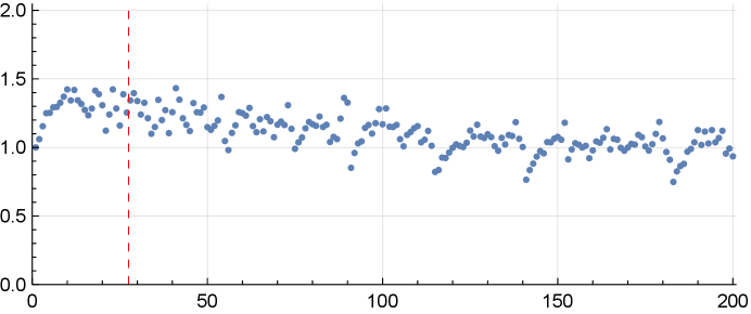
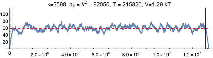
From these images, it seems apparent that one should focus more on than . In Figure 7 we show four plots of , with the average value as a red dashed horizontal line, and , as vertical black lines. The four, which appear to be typical, show that is fairly smooth between and . In fact, about half of arises from and . Figure 8 shows the proportion of that arises from the edge values of .


3 The BFR Gambit
In [BFR], a small variance (which arose by way of an inequality from coding theory, and a rephrasing of the Erdős-Turán argument in terms of degree sequences of hypergraphs) was used to imply a lumpiness in the difference set. This lumpiness was then used to supercharge a proof of Lindström’s, yielding
It is, as the proven value was rounded up to , equivalent to
This work was the first real improvement in the bounds, upper or lower, of since 1941. It was the direct inspiration for the current work.
We play the same gambit, but exploit the phenomenon in a different way. Instead of using the Lindström proof, we re-use Theorem 4 on a subset of . That is, either has a large variance (and so a large diameter), or a large subset has a difference set that does not include many small values, and so the small diffs is large, forcing to have a large diameter.
3.1 A Toy Version of our Argument
In this short subsection, we give a simple argument using the Erdős-Turán Sidon Set Equation to prove that . In the next subsection, we engage in a somewhat harder-to-optimize version of this argument with more parameters that leads to a better bound on than that given in BFR.
Normalize as above, so that , and set (it needs to be an integer, but we will ignore this issue in this subsection, and we shall also be cavalier about inequalities that may only hold for sufficiently large ). For positive , set and , and let , the average value of for . If , then . We begin by considering as a function of ; it is monotone increasing for . Set
If , then
Now suppose that , so that . Set
Clearly
Set and . By the definition of , we see that
We also see that has pairs of elements whose difference is at most . We have
differences, each at most . Set , which is larger than , so that
To get better numbers, we should have more levels than just , and we should allow to vary. We pursue this in the next subsection.
3.2 More Parameters Leads to a Better Bound
We begin by fixing real numbers , , , , . Specific values that work out well are:
| (6) | ||||
| (7) | ||||
| (8) | ||||
| (9) | ||||
| (10) |
The reason for the ridiculous value of is to make two bounds we will encounter exactly equal.
To better wrangle the equations, set , , (all of the variables are chosen in to make some other variable an integer), and , and assume that , so that .
For , we have . For negative subscripts, we set . For example, and . As a function of , we see that is nondecreasing for , and increases by at most 1 as increases by 1.

We partition the interval into 5 parts:111Setting forces , and is thereby substantially simpler, but leads merely .
We set by , and set . For example, and .
Claim 1.
If , then .
Proof of Claim:.
By hypothesis of this claim, , and so . ∎
Claim 2.
If , then
Proof of Claim:.
We now work under the hypothesis that . Note that , so that necessarily is not empty. It can happen that are empty.
Let be the set of positive differences of elements of . In particular, if is a subset of a Sidon set, then . We set
We will find that , but that if are small then is missing a substantial number of small integers, so that is , which forces the diameter of to be large. This, in turn, forces to be large, and this gives a bound on .
Claim 3.
Suppose that . Then .
Proof of Claim:.
As , we know that is nonempty. Let . By the definition of , we know that . Therefore,
∎
We set and . Note that are disjoint, and disjoint from . But they are all subsets of the Sidon set , so any difference in or is necessarily missing from , and so contributes to (provided is large enough).
Claim 4.
Suppose that .
There are at least elements of , each at most .
There are at least elements of , each at most .
There are at least elements of , each at most .
Proof of Claim:.
We note that and the definition of (together with the nonemptiness of , which is implied by ) gives
and so
Similarly,
For a Sidon set , the size of is exactly . For example, has
elements, each at most , which is at most .
Essentially identical computations give the other assertions of this claim. ∎
We set , with chosen to make an integer.
Claim 5.
Suppose that and . Then is at least , where
| (11) | ||||
| (12) |
Proof of Claim:.
By hypothesis, , so all of the differences described in Claim 4 contribute to
For example, the differences in contribute at least
| (13) |
to . Similarly, the
differences in , each at most , contribute at least
| (14) |
to . Finally, and have many differences that haven’t been counted already. They have
elements, but only
each at most , have not been accounted for already. These contribute an additional
| (15) |
to . After some algebra to rearrange terms, this claim is confirmed. ∎
Claim 6.
Suppose that . Then
Proof.
We begin with
where we have used Theorem 4 and Claim 5. The first term contributes to the coefficient, and the last term contributes . The middle term can be converted to a geometric series:
Defining by , we get
Thus,
| (16) |
From Claim 3, we know that is at most . The right side of (16) is a linear expression in and , which we must maximize in the region . The maximum occurs222Ideally, we would set and then this expression has a factor of , which we could replace with . The author didn’t realize this until after the optimization work was complete, and including it would make some intermediate optimization steps more delicate. at the vertex , and is
∎
Claim 2 and Claim 6 complete the proof of Theorem 2. The value of was chosen so as to make the two bounds exactly equal. In general, one sets
to accomplish this.
In reality, the bounds were first worked out symbolically using Mathematica, and then optimized using simulated annealing. Having good estimates of where the optimal value occurs then allowed certain streamlining of the argument.
Acknowledgements
I wish to thank Melvyn B. Nathanson and Yin Choi Cheng, who independently showed great patience while I explained early versions of this work.
The author is supported by a PSC–CUNY Award, jointly funded by The Professional Staff Congress and The City University of New York.