On the role of vorticity stretching and strain self-amplification in the turbulence energy cascade

In this paper, the kinetic energy cascade is quantified via direct numerical simulation (DNS) of forced homogeneous isotropic turbulence (HIT) in a triply periodic domain. The incompressible Navier-Stokes equations,

$$\frac{\partial u_{i}}{\partial t}+u_{j}\frac{\partial u_{i}}{\partial x_{j}}=-\frac{\partial p}{\partial x_{i}}+\nu\nabla^{2}u_{i}+f_{i},\hskip 21.68231pt\frac{\partial u_{j}}{\partial x_{j}}=0,$$

(1)

are solved using a pseudo-spectral method with $1024$ collocation points in each direction. The velocity field, $\mathbf{u}$, is advanced in time with a second-order Adams-Bashforth scheme, and the pressure $p$ simply enforces the divergence-free condition. The $2\sqrt{2}/3$ rule for wave number truncation is used with phase-shift dealiasing (Patterson & Orszag, 1971). The forcing, $\mathbf{f}$, is specifically designed to maintain constant kinetic energy in the first two wave number shells.

The simulation was initialized using a Gaussian random velocity field satisfying a model turbulent energy spectrum. The simulation was first run through a startup period to reach statistical stationarity. Then, statistics are computed over $6$ large-eddy turnover times. The Taylor-scale Reynolds number is approximately $Re_{\lambda}=400$ with grid resolution $k_{\max}\eta=1.4$. The integral length scale is about $20\%$ of the periodic box size of $2\pi$ and $L/\eta=460$. The skewness of the longitudinal velocity gradient is $-0.58$, and the flatness of the longitudinal and transverse velocity gradients are $8.0$ and $12.4$, respectively, in reasonable agreement with previous simulations (Ishihara et al., 2007).

HIT is a very useful canonical flow to efficiently explore the energetics of small- and intermediate-scale turbulence dynamics. The analysis performed in this paper is not limited to HIT in principle, and the inertial range results are expected to be representative of a wide range of turbulent shear flows at sufficiently high Reynolds numbers.

Vorticity stretching and strain self-amplification are dynamical processes defined via the velocity gradient tensor,

$$A_{ij}=\frac{\partial u_{i}}{\partial x_{j}}=S_{ij}+\Omega_{ij},\hskip 21.68231ptS_{ij}=\frac{1}{2}\left(A_{ij}+A_{ji}\right),\hskip 21.68231pt\Omega_{ij}=\frac{1}{2}\left(A_{ij}-A_{ji}\right).$$

(2)

The velocity gradient in three dimensions is a $3\times 3$ tensor describing the variation of the three velocity components in each of the three coordinate directions. It is comprised of the strain-rate tensor, $\mathbf{S}$, which describes the rate at which fluid particles are undergoing deformation, and the rotation-rate tensor, $\boldsymbol{\Omega}$, which describes the rate at which fluid particles are undergoing solid body rotation. Mathematically speaking, the strain-rate and rotation-rate tensors are the symmetric and anti-symmetric parts of the velocity gradient tensor, respectively.

The decomposition of $\mathbf{A}$ into $\mathbf{S}$ and $\boldsymbol{\Omega}$ is foundational to the energetics of turbulent flows because viscosity resists deformation but not rotation. Thus, the rate at which kinetic energy is dissipated into thermal energy depends only on the (Frobenius norm of the) strain-rate tensor,

$$\epsilon=2\nu S_{ij}S_{ij}=2\nu\|\mathbf{S}\|^{2}.$$

(3)

On the other hand, the rotation-rate tensor, which may be written in terms of the vorticity vector $\boldsymbol{\omega}$,

$$\Omega_{ij}=-\frac{1}{2}\epsilon_{ijk}\omega_{k},\hskip 21.68231pt\omega_{i}=-\epsilon_{ijk}\Omega_{jk},$$

(4)

plays no direct role in the viscous dissipation of kinetic energy. However, vorticity is still essential to the dynamics of energy dissipation, as may be seen from the first relation of Betchov (1956) for incompressible homogeneous turbulence,

$$\langle\|\mathbf{S}\|^{2}\rangle=\frac{1}{2}\langle|\boldsymbol{\omega}|^{2}\rangle.$$

(5)

Angle brackets denote ensemble averaging. The Betchov relation shows that the average (or global) amount of vorticity and strain-rate is held in balance for incompressible flows, presumably by the action of the pressure as it enforces $\nabla\cdot\mathbf{u}=0$. Thus, the significantly enhanced dissipation rates in turbulence cannot occur without equally enhanced enstrophy. At sufficiently high Reynolds numbers, this relationship holds to good approximation even for inhomogeneous flows.

For this reason, it is useful to consider (one half of) the norm of the full velocity gradient tensor,

$$\frac{1}{2}\|\mathbf{A}\|^{2}=\frac{1}{4}|\boldsymbol{\omega}|^{2}+\frac{1}{2}\|\mathbf{S}\|^{2}$$

(6)

when considering the mean rate of dissipation. Statistically, the velocity gradient magnitude is equi-partitioned between enstrophy and dissipation. Thus, the second invariant of the velocity gradient tensor,

$$Q=-\frac{1}{2}A_{ij}A_{ji}=\frac{1}{4}|\boldsymbol{\omega}|^{2}-\frac{1}{2}\|\mathbf{S}\|^{2},$$

(7)

has an average of zero.

The strain-rate tensor, being symmetric, has 3 real eigenvalues, $\lambda_{1}>\lambda_{2}>\lambda_{3}$, associated with a set of orthogonal eigenvectors. The eigenvalues sum to zero for incompressible flows, $\lambda_{1}+\lambda_{2}+\lambda_{3}=0$. Therefore, the largest eigenvalue is always extensional along its eigenvector, $\lambda_{1}\geq 0$, and the smallest one is always compressive, $\lambda_{3}\leq 0$. The intermediate eigenvalue, $\lambda_{2}$, may be positive or negative. The sign of $\lambda_{2}$ indicates the topology of fluid particle deformations, Figure 3, and has more important dynamical effects as discussed below.

Consider a Lagrangian view of turbulence as a collection of fluid particles characterized by their deformational and rotational behavior, i.e., their velocity gradient tensor. The Lagrangian evolution equation for the velocity gradient tensor is derived as the gradient of Eq. (1),

$$\frac{DA_{ij}}{Dt}\equiv\frac{\partial A_{ij}}{\partial t}+u_{k}\frac{\partial A_{ij}}{\partial x_{k}}=-A_{ik}A_{kj}-\frac{\partial^{2}p}{\partial x_{i}\partial x_{j}}+\nu\nabla^{2}A_{ij}+\frac{\partial f_{i}}{\partial x_{j}}.$$

(8)

For HIT simulations with large-scale forcing, the gradient of the force is typically negligible compared to other terms in Eq. (8) at high Reynolds numbers. The first term on the right side of Eq. (8), $A_{ik}A_{kj}$, contains the dynamical mechanisms of interest: vorticity stretching/tilting/compressing and strain self-amplification/attenuation. The second term on the right side of Eq. (8) is the pressure Hessian tensor. It may be split into local and nonlocal parts, i.e., the isotropic and deviatoric parts, respectively (Ohkitani & Kishiba, 1995),

$$\frac{\partial^{2}p}{\partial x_{i}\partial x_{j}}(\mathbf{x})=\underbrace{\frac{2}{3}Q(\mathbf{x})\delta_{ij}}_{\text{isotropic, local}}+\underbrace{\iiint_{P.V.}d\mathbf{r}~{}\frac{Q(\mathbf{x}+\mathbf{r})}{2\pi|\mathbf{r}|^{3}}\left(\delta_{ij}-3\frac{r_{i}r_{j}}{|\mathbf{r}|^{2}}\right)}_{\text{deviatoric, nonlocal}}.$$

(9)

The isotropic part of this tensor is given by the pressure Poisson equation (from the divergence of Eq. (1)),

$$\nabla^{2}p=2Q,$$

(10)

which is the equation locally enforcing the divergence free condition along the Lagrangian trajectory. The deviatoric part of the pressure Hessian, given by the nonlocal integral in Eq. (9), represents the action of the pressure to enforce $\nabla\cdot\mathbf{u}=0$ at nearby points in the flow. Splitting the pressure Hessian in this way enables a decomposition of the Lagrangian velocity gradient evolution, Eq. (8), into the autonomous dynamics of a fluid particle and the influence of other nearby fluid particles,

$$\frac{DA_{ij}}{Dt}=-\underbrace{\left(A_{ik}A_{kj}-\frac{1}{3}A_{mn}A_{nm}\delta_{ij}\right)}_{\text{autonomous dynamics}}-\underbrace{\left(\frac{\partial^{2}p}{\partial x_{i}x_{j}}-\frac{1}{3}\nabla^{2}p\delta_{ij}\right)+\nu\nabla^{2}A_{ij}}_{\text{nearby particle interactions}}.$$

(11)

Significant insight may be gained into velocity gradient dynamics by focusing on its autonomous dynamics using the restricted Euler equation,

$$\frac{DA_{ij}}{Dt}=-A_{ik}A_{kj}-\frac{1}{3}A_{mn}A_{nm}\delta_{ij}.$$

(12)

By neglecting the interaction with the velocity gradients of other surrounding fluid particles, the restricted Euler equation represents a dramatic mathematical simplification of turbulent flows while retaining some key dynamical processes. In fact, rigorous mathematical results are possible (Vieillefosse, 1982, 1984; Cantwell, 1992).

The most salient feature of solutions to the restricted Euler equation is a finite-time singularity for (almost) all initial conditions. The cause of this singularity may be readily seen by considering the equation for the velocity gradient norm in restricted Euler dynamics,

$$\frac{D}{Dt}\left(\frac{1}{2}\|\mathbf{A}\|^{2}\right)=\frac{1}{4}\omega_{i}S_{ij}\omega_{j}-S_{ij}S_{jk}S_{ki}.$$

(13)

The two terms on the right side of Eq. (13) represent production of velocity gradient magnitude by vorticity stretching and strain self-amplification, respectively.

The local rate of velocity gradient production by vorticity stretching/compression,

$$P_{\omega}=\frac{1}{4}\omega_{i}S_{ij}\omega_{j}=\frac{1}{4}|\boldsymbol{\omega}|^{2}\sum_{i=1}^{3}\lambda_{i}\cos^{2}(\theta_{\omega,i}),$$

(14)

depends strongly on how the vorticity vector aligns in the strain-rate eigenframe, Figure 3. Here, $\theta_{\omega,i}$ is the angle between the vorticity and the i^th eigenvector of the strain-rate tensor. The local enstrophy, and hence the velocity gradient magnitude, is increased when the vorticity vector aligns more with eigenvectors having positive (extensional) eigenvalues. Velocity gradient production rate via strain self-amplification is,

$$P_{s}=-S_{ij}S_{jk}S_{ki}=-3\lambda_{1}\lambda_{2}\lambda_{3}.$$

(15)

The strain-rate amplifies itself when $\lambda_{2}>0$ but self-attenuates when $\lambda_{2}<0$. It is no surprise, then, that restricted Euler solutions tend toward a state with two positive strain-rate eigenvalues, $\lambda_{1}=\lambda_{2}=-\frac{1}{2}\lambda_{3}$, as they approach the finite-time singularity. Furthermore, the vorticity aligns with the eigenvector associated with the intermediate eigenvalue, $\lambda_{2}$, in this approach to singularity. Thus, both strain self-amplification and vorticity stretching together drive the finite-time singularity in restricted Euler.

However, strain self-amplification dominates vorticity stretching in the restricted Euler singularity, as can be demonstrated by considering the dynamics in terms of the second and third invariants. The second invariant, $Q$, is defined in Eq. (7) as the difference between the square magnitudes of vorticity and strain-rate. The third invariant,

$$R=-\frac{1}{3}A_{ij}A_{jk}A_{ki}=-\frac{1}{3}S_{ij}S_{jk}S_{ki}-\frac{1}{4}\omega_{i}S_{ij}\omega_{j}=\frac{1}{3}P_{s}-P_{\omega}$$

(16)

is the difference between (one third of) the strain self-amplification rate and the vorticity stretching rate. The restricted Euler equation may be written in terms of $Q$ and $R$ as

$$\frac{DQ}{Dt}=-3R,\hskip 21.68231pt\frac{DR}{Dt}=\frac{2}{3}Q^{2}.$$

(17)

Thus, $DR/Dt\geq 0$ always. Restricted Euler solutions evolve toward positive $R$ which is characterized by more strain self-amplification than vorticity stretching. Vela-Martín & Jiménez (2020) illuminates a subset of this behavior by looking at the dynamics of $\lambda_{2}$. Further, as $R$ becomes positive, $DQ/Dt<0$ and the second invariant decreases. The result is that the finite-time singularities in restricted Euler solutions are characterized by $R\gg 0$ and $Q\ll 0$. That is, the strain-rate blows up faster than the vorticity.

Incompressible Navier-Stokes dynamics, with the nonlocal pressure Hessian and viscous term reintroduced, do not exhibit the finite-time singularity seen for the restricted Euler equation. Instead, there is a balance between vorticity and strain-rate as already discussed with Eq. (5). Betchov (1956) provided another relation for incompressible homogeneous turbulence, namely,

$$-\langle S_{ij}S_{jk}S_{ki}\rangle=\frac{3}{4}\langle\omega_{i}S_{ij}\omega_{j}\rangle,\hskip 21.68231pt\text{or}\hskip 21.68231pt\langle P_{s}\rangle=3\langle P_{\omega}\rangle,$$

(18)

which means that the average value of $R$ is also zero, as enforced by the pressure via the constraint $\nabla\cdot\mathbf{u}=0$. As with Eq. (5), Eq. (18) is approximately true for high Reynolds number inhomogeneous flows. What this means is that, while the pressure enforces an equal partition between dissipation and enstrophy, it also enforces that the strain-rate self-amplification produces stronger velocity gradients at three times the rate of vorticity stretching.

The significance of the restricted Euler equation is that its signature features are unmistakably observed in the statistics of experiments and direct numerical simulations of the Navier-Stokes equations. Indeed, turbulent flows show a tendency of the vorticity to align with the strain-rate eigenvector associated with the intermediate eigenvalue, $\lambda_{2}$, which tends to be positive much more often than it is negative (Kerr, 1987; Ashurst et al., 1987; Tsinober et al., 1992; Lund & Rogers, 1994; Mullin & Dahm, 2006; Gulitski et al., 2007). Note that the alignment of vorticity is similar to, but slightly different from, the alignment of material lines in a turbulent flow (Luthi et al., 2005; Holzner et al., 2010; Johnson & Meneveau, 2016; Johnson et al., 2017), a subtle point to remember in the context of Taylor (1938). An important difference between vorticity and material lines is that the vorticity is an active feedback on the strain-rate and evolves on the same time scale, so that while the vorticity typically tilts toward the strain-rates most stretching eigenvalue, it is more successful in aligning with direction in which that eigenvector previously pointed (Xu et al., 2011). In addition, turbulence is characterized by enhanced probabilities of strong velocity gradients along the Vieillefosse manifold, $4Q^{3}+27R^{2}=0$ in the fourth quadrant, which is an attracting manifold along which the finite-time singularity occurs for restricted Euler (Cantwell, 1993; Soria et al., 1994; Chong et al., 1998; Nomura & Post, 1998; Ooi et al., 1999; Gulitski et al., 2007; Elsinga & Marusic, 2010). While the nonlocal part of the pressure Hessian tensor, along with viscous effects, are important for describing turbulence quantitatively, many of the unique qualitative features of turbulent velocity gradients can be connected to restricted Euler dynamics.

In summary, velocity gradients in a fluid undergoing nonlinear self-advection ($\mathbf{u}\cdot\nabla\mathbf{u}$) naturally strengthen via vorticity stretching and strain self-amplification. Of these two dynamical processes, strain self-amplification is three times as strong on average, as enforced by the non-local action of the pressure. For more discussion about velocity gradient dynamics, as well as measurement and modelling, the reader is referred to (Wallace, 2009; Tsinober, 2009; Meneveau, 2011). Next, the energy cascade is introduced using a spatial filtering formulation. As will be shown, this framework allows for directly relating velocity gradient dynamics to the energy cascade.

A spatial low-pass filter,

$$\overline{a}^{\ell}(\mathbf{x})=\iiint d\mathbf{r}~{}G_{\ell}(\mathbf{r})a(\mathbf{x}+\mathbf{r}),\hskip 21.68231pt\widehat{\overline{a}^{\ell}}(\mathbf{k})=\widehat{G_{\ell}}(\mathbf{k})\widehat{a}(\mathbf{k})$$

(19)

retains features of a field $a(\mathbf{x})$ that are larger than $\ell$ while removing features smaller than $\ell$ (Leonard, 1975; Germano, 1992). An example velocity field from the DNS of HIT is shown in Figure 4, before and after the application of a spatial filter. The spatial filter may be interpreted as a form of local averaging, weighted by the filter kernal $G_{\ell}(\mathbf{r})$. Following Germano (1992), the generalized second moment is the difference of the filtered product and the product of two filtered fields,

$$\tau_{\ell}(a,b)=\overline{ab}^{\ell}-\overline{a}^{\ell}\overline{b}^{\ell}.$$

(20)

It is a generalized covariance of small-scale activity (smaller than $\ell$).

The kinetic energy can be thus defined as the sum of large-scale and small-scale energies,

$$\tfrac{1}{2}\overline{u_{i}u_{i}}^{\ell}=\tfrac{1}{2}\overline{u}_{i}^{\ell}\overline{u}_{i}^{\ell}+\tfrac{1}{2}\tau_{\ell}(u_{i},u_{i}).$$

(21)

If the filter kernel is positive semi-definite, i.e., $G_{\ell}(\mathbf{r})\geq 0$ for all $\mathbf{r}$, then the subfilter-scale energy is positive everywhere, $\tau(u_{i},u_{i})(\mathbf{x})\geq 0$ for all $\mathbf{x}$ (Vreman et al., 1994).

Applying a low-pass filter to the incompressible Navier-Stokes equations, Eq. (1), results in an evolution equation for the filtered velocity field,

$$\frac{\partial\overline{u}_{i}^{\ell}}{\partial t}+\overline{u}_{j}^{\ell}\frac{\partial\overline{u}_{i}^{\ell}}{\partial x_{j}}=-\frac{\partial\overline{p}^{\ell}}{\partial x_{i}}+\nu\nabla^{2}\overline{u}_{i}^{\ell}-\frac{\partial\tau_{\ell}(u_{i},u_{j})}{\partial x_{j}}+\overline{f}_{i}^{\ell}.$$

(22)

The main difference with the unfiltered Navier-Stokes equation, Eq. (1), is the introduction of the subfilter stress tensor’s divergence on the right side. The dynamical equation for the large-scale kinetic energy directly follows from multiplication of Eq. (22) by $\overline{u}_{i}^{\ell}$,

$$\frac{\partial\left(\tfrac{1}{2}\overline{u}_{i}^{\ell}\overline{u}_{i}^{\ell}\right)}{\partial t}+\frac{\partial\Phi_{j}^{\ell}}{\partial x_{j}}=\overline{u}_{i}^{\ell}\overline{f}_{i}^{\ell}+\tau_{\ell}(u_{i},u_{j})\overline{S}_{ij}^{\ell}-2\nu\overline{S}_{ij}^{\ell}\overline{S}_{ij}^{\ell},$$

(23)

$$\text{where}\hskip 21.68231pt\Phi_{j}^{\ell}=\tfrac{1}{2}\overline{u}_{i}^{\ell}\overline{u}_{i}^{\ell}\overline{u}_{j}^{\ell}+\overline{p}^{\ell}\overline{u}_{j}^{\ell}-2\nu\overline{u}_{i}^{\ell}\overline{S}_{ij}^{\ell}+\overline{u}_{i}^{\ell}\tau_{\ell}(u_{i},u_{j}).$$

The spatial transport of large-scale kinetic energy, $\boldsymbol{\Phi}^{\ell}$, occurs due to (i) advection by large-scale motions, $\tfrac{1}{2}\overline{u}_{i}^{\ell}\overline{u}_{i}^{\ell}\overline{u}_{j}^{\ell}$, (ii) large-scale pressure transport, $\overline{p}^{\ell}\overline{u}_{j}^{\ell}$, (iii) viscous diffusion, $-2\nu\overline{u}_{i}^{\ell}\overline{S}_{ij}^{\ell}$, and (iv) mixing by subfilter-scale motions $\overline{u}_{i}^{\ell}\tau_{\ell}(u_{i},u_{j})$.

More importantly for the present topic, there are three source/sink terms. First, large-scale kinetic energy is produced though work done by the applied forcing function, $\overline{u}_{i}^{\ell}\overline{f}_{i}^{\ell}$. Second, the subfilter stress may add or remove energy depending on its alignment with the filtered strain-rate tensor, $\tau_{\ell}(u_{i},u_{j})\overline{S}_{ij}^{\ell}$. Finally, the direct dissipation of large-scale kinetic energy by viscosity, $-2\nu\overline{S}_{ij}^{\ell}\overline{S}_{ij}^{\ell}$, is typically negligible if $\ell\gg\eta$.

An equation for total kinetic energy, $\tfrac{1}{2}\overline{u_{i}u_{i}}^{\ell}$, is constructed by multiplying Eq. (1) by $u_{i}$ and then filtering. Equation (23) is subtracted from the resulting equation to form the transport equation for the small-scale energy,

$$\frac{\partial\left(\tfrac{1}{2}\tau_{\ell}(u_{i},u_{j})\right)}{\partial t}+\frac{\partial\phi_{j}^{\ell}}{\partial x_{j}}=\tau_{\ell}\left(u_{i},f_{i}\right)-\tau_{\ell}\left(u_{i},u_{j}\right)\overline{S}_{ij}^{\ell}-2\nu~{}\tau_{\ell}\left(S_{ij},S_{ij}\right),$$

(24)

$$\text{where}\hskip 21.68231pt\phi_{j}^{\ell}=\tfrac{1}{2}\tau_{\ell}\left(u_{i},u_{i}\right)\overline{u}_{j}^{\ell}+\tfrac{1}{2}\tau_{\ell}\left(u_{i},u_{i},u_{j}\right)+\tau_{\ell}\left(p,u_{j}\right)-2\nu~{}\tau_{\ell}\left(u_{i},S_{ij}\right).$$

Spatial transport of small-scale kinetic energy, $\boldsymbol{\phi}^{\ell}$, is done by (i) large-scale advection, $\tfrac{1}{2}\tau_{\ell}\left(u_{i},u_{i}\right)\overline{u}_{j}$, (ii) small-scale mixing, $\tfrac{1}{2}\tau_{\ell}\left(u_{i},u_{i},u_{j}\right)$, (iii) small-scale pressure transport, $\tau_{\ell}\left(p,u_{j}\right)$, and (iv) viscous diffusion, $2\nu~{}\tau_{\ell}\left(u_{i},S_{ij}\right)$. The second transport term is a generalized third moment (Germano, 1992),

$$\tau_{\ell}(a,b,c)=\overline{abc}^{\ell}-\overline{a}^{\ell}\tau_{\ell}(b,c)-\overline{b}^{\ell}\tau_{\ell}(a,c)-\overline{c}^{\ell}\tau_{\ell}(a,b)-\overline{a}^{\ell}\overline{b}^{\ell}\overline{c}^{\ell}.$$

(25)

There are three sources/sinks in Eq. (24), which have the following significance. The first source is direct forcing of the small scales, $\tau_{\ell}\left(u_{i},f_{i}\right)$, which is typically negligible for $\ell\ll L$. The second is the same term, $-\tau_{\ell}\left(u_{i},u_{j}\right)\overline{S}_{ij}^{\ell}$, as appears with opposite sign in the large-scale energy equation, Eq. (23). This term represents the rate at which energy is transferred from motions of size larger than $\ell$ to motions of size smaller than $\ell$. Thus, the energy cascade rate is defined as (Leonard, 1975; Germano, 1992; Meneveau & Katz, 2000),

$$\Pi^{\ell}=-\mathring{\tau}_{\ell}\left(u_{i},u_{j}\right)\overline{S}_{ij}^{\ell},$$

(26)

where the overset circle indicates the deviatoric component of the tensor,

$$\mathring{\tau}_{\ell}(u_{i},u_{j})=\tau_{\ell}(u_{i},u_{j})-\tfrac{1}{3}\tau_{\ell}(u_{k},u_{k})\delta_{ij}.$$

(27)

The isotropic part of the subfilter stress tensor does not contribute to the energy cascade rate, $\Pi^{\ell}$, because the trace of $\overline{\mathbf{S}}^{\ell}$ is zero due to incompressibility. Positive cascade rate indicates energy transfer from large to small scales and negative rate indicates backscatter or inverse cascade. It may be interpreted as the rate at which large-scale motions do work on small-scale motions (Ballouz & Ouellette, 2018).

The sign of $\Pi^{\ell}$ depends on how the eigenvectors of the subfilter stress tensor aligns with those of the filtered strain-rate tensor (Ballouz & Ouellette, 2020). This may be made explicit by writing the cascade rate in terms of eigenvalues of the filtered strain-rate, $\lambda_{i}$, and deviatoric subfilter stress tensor, $\mu_{j}$,

$$\Pi^{\ell}=\sum_{i=1}^{3}\sum_{j=1}^{3}\lambda_{i}^{\ell}\mu_{j}^{\ell}\cos^{2}(\theta_{ij}^{\ell}).$$

(28)

Here, $\theta_{ij}$ is the angle between the i^th eigenvector of the filtered strain-rate and j^th eigenvector of the subfilter stress tensor.

Averaging Eqs. (23) and (24) for a stationary, homogeneous flow yields, respectively,

$$0=\left\langle\overline{u}_{i}^{\ell}\overline{f}_{i}^{\ell}\right\rangle+\left\langle\tau_{\ell}(u_{i},u_{j})\overline{S}_{ij}^{\ell}\right\rangle-2\nu\left\langle\overline{S}_{ij}^{\ell}\overline{S}_{ij}^{\ell}\right\rangle,$$

(29)

$$0=\left\langle\tau_{\ell}\left(u_{i},f_{i}\right)\right\rangle-\left\langle\tau_{\ell}\left(u_{i},u_{j}\right)\overline{S}_{ij}^{\ell}\right\rangle-2\nu\left\langle\tau_{\ell}\left(S_{ij},S_{ij}\right)\right\rangle.$$

(30)

In the inertial range of turbulence, $\eta\ll\ell\ll L$, the viscous dissipation of the large scales and forcing of the small scales may be neglected,

$$\left\langle u_{i}f_{i}\right\rangle\approx\left\langle\overline{u}_{i}^{\ell}\overline{f}_{i}^{\ell}\right\rangle\approx-\left\langle\tau_{\ell}(u_{i},u_{j})\overline{S}_{ij}^{\ell}\right\rangle\approx 2\nu\left\langle\tau_{\ell}\left(S_{ij},S_{ij}\right)\right\rangle\approx 2\nu\left\langle S_{ij}S_{ij}\right\rangle.$$

(31)

More simply, the inertial range is the range length scales, $\ell$, for which $\left\langle\Pi\right\rangle\approx\left\langle\epsilon\right\rangle$. Figure 5a tests for scales where this relation approximately holds.

Velocity increments,

$$\delta u_{i}(\mathbf{r};\mathbf{x})=u_{i}(\mathbf{x}+\mathbf{r})-u_{i}(\mathbf{x})$$

(32)

and structure functions are one of the prominent tools of classical turbulence theory. Filtered velocity gradients are intimately related to velocity increments (Eyink, 1995),

$$\overline{A}_{ij}^{\ell}(\mathbf{x})\equiv\frac{\partial\overline{u}_{i}}{\partial x_{j}}(\mathbf{x})=\iiint d\mathbf{r}~{}\left.\frac{\partial G}{\partial r_{j}}\right|_{\mathbf{r}}\delta u_{i}(\mathbf{r},\mathbf{x})=\int_{0}^{\infty}d\rho~{}\frac{dG}{d\rho}\left[\oiint dS~{}\frac{r_{j}}{|\mathbf{r}|}\delta u_{i}(\mathbf{r};\mathbf{x})\right]$$

(33)

where the filter kernel is assumed to be spherically symmetric. That is, the filtered velocity gradient is an averaging of velocity increments weighted by the gradient of the filter kernel. For a top-hat filter kernel, the gradient of the filter kernel is a Dirac delta function, so the filtered velocity gradient components are directionally-weighted averages of velocity increments on a spherical shell at $|\mathbf{r}|=\ell$. Velocity gradients for other filter kernel shapes also average across increments $|\mathbf{r}|$ near $\ell$. Thus, the scaling of filtered velocity gradients in the inertial range can be deduced from the scaling of velocity increments,

$$\|\overline{\mathbf{A}}^{\ell}\|\sim\frac{\delta u}{\ell}\sim\ell^{-2/3},$$

(34)

modulo intermittency corrections. Filtered velocity gradients contain information about velocity increments in the flow, arranged so as to illuminate the local topology of the flow at scale $\ell$. That is, filtered velocity gradients can be decomposed into rotation and deformation by considering the filtered vorticity vector and filtered strain-rate tensor,

$$\overline{A}_{ij}^{\ell}=\overline{S}_{ij}^{\ell}+\overline{\Omega}_{ij}^{\ell},\hskip 21.68231pt\overline{S}_{ij}^{\ell}=\frac{1}{2}\left(\overline{A}_{ij}^{\ell}+\overline{A}_{ji}^{\ell}\right),\hskip 21.68231pt\overline{\Omega}_{ij}^{\ell}=\frac{1}{2}\left(\overline{A}_{ij}^{\ell}-\overline{A}_{ji}^{\ell}\right),$$

(35)

$$\overline{\Omega}_{ij}^{\ell}=-\frac{1}{2}\epsilon_{ijk}\overline{\omega}_{k}^{\ell},\hskip 21.68231pt\overline{\omega}_{i}^{\ell}=-\epsilon_{ijk}\overline{\Omega}_{jk}^{\ell},$$

(36)

$$\frac{1}{2}\|\overline{\mathbf{A}}^{\ell}\|^{2}=\frac{1}{4}|\overline{\boldsymbol{\omega}}^{\ell}|^{2}+\frac{1}{2}\|\overline{\mathbf{S}}^{\ell}\|^{2},\hskip 21.68231pt\left\langle\|\overline{\mathbf{S}}^{\ell}\|^{2}\right\rangle=\frac{1}{2}\left\langle|\overline{\boldsymbol{\omega}}^{\ell}|^{2}\right\rangle$$

(37)

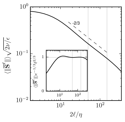
The power-law scaling of the filtered strain-rate norm is shown in Figure 5b as another indication of what filter widths may be considered to be in the inertial range.

Figure 6 shows vorticity and filtered vorticity fields from the same snapshot used for Figure 4. It is evident that the vorticity is predominantly organized at the smallest scales of motion, near $\eta$. This is true of the velocity gradient tensor in general. However, the filtered velocity gradient, as demonstrated for the filtered vorticity, is primarily organized at a scale near the filter width. Thus, the filtered velocity gradient provides a good definition of fluid motions at scale $\ell$.

Like the filtered velocity gradient, the subfilter stress tensor may also be written as a local averaging of velocity increments (Constantin et al., 1994; Eyink, 1995),

$$\tau_{\ell}(u_{i},u_{j})=\left[\iiint d\mathbf{r}~{}G_{\ell}(\mathbf{r})\delta u_{i}(\mathbf{r};\mathbf{x})\delta u_{j}(\mathbf{r};\mathbf{x})\right]\\ -\left[\iiint d\mathbf{r}~{}G_{\ell}(\mathbf{r})\delta u_{i}(\mathbf{r};\mathbf{x})\right]\left[\iiint d\mathbf{r}~{}G_{\ell}(\mathbf{r})\delta u_{j}(\mathbf{r};\mathbf{x})\right].$$

(38)

In this way, it can be directly shown that

$$\tau_{\ell}(u_{i},u_{j})\sim\delta u^{2},\hskip 13.00806pt\text{and}\hskip 13.00806pt\overline{S}_{ij}^{\ell}\sim\delta u/\ell,\hskip 13.00806pt\text{therefore}\hskip 13.00806pt\Pi^{\ell}\sim\delta u^{3}/\ell$$

(39)

so that the inertial range equation, from Eq. (31), in the form $\langle\Pi^{\ell}\rangle=\langle\epsilon\rangle$ is in some ways analogous to the celebrated four-fifths law of Kolmogorov (1941a), i.e., $\langle\delta u_{L}^{3}(r)\rangle=-\tfrac{4}{5}\langle\epsilon\rangle r$. The similarity between these two is highlighted in Figure 5a, which includes the pre-multiplied third-order longitudinal structure function alongside $\langle\Pi\rangle/\langle\epsilon\rangle$. These two are similar diagnostics of inertial range scales.

Definitively linking the energy cascade rate with vorticity stretching and strain self-amplification is naturally done by considering the dynamics of filtered velocity gradients. The gradient of filtered Navier-Stokes, Eq. (22),

$$\frac{\overline{D}~{}\overline{A}_{ij}^{\ell}}{\overline{Dt}}=-\underbrace{\left(\overline{A}_{ik}^{\ell}\overline{A}_{kj}^{\ell}-\frac{1}{3}\overline{A}_{mn}^{\ell}\overline{A}_{nm}^{\ell}\delta_{ij}\right)}_{\text{autonomous dynamics}}-\left(\frac{\partial^{2}\overline{p}^{\ell}}{\partial x_{i}x_{j}}-\frac{1}{3}\nabla^{2}\overline{p}^{\ell}\delta_{ij}\right)+\nu\nabla^{2}\overline{A}_{ij}^{\ell}-\frac{\partial\tau_{\ell}(u_{i},u_{k})}{\partial x_{j}\partial x_{k}}$$

(40)

gives the dynamical evolution of filtered velocity gradients along filtered Lagrangian trajectories, $\overline{D}/\overline{Dt}=\partial/\partial t+\overline{\mathbf{u}}^{\ell}\cdot\nabla$. The difference from unfiltered velocity gradients, Eq. (11), is the gradient of the subfilter scale force. The dynamical consequence of the subfilter scale force is subtle, and the restricted Euler-like features observed for unfiltered velocity gradients are also seen for filtered ones (Danish & Meneveau, 2018). In other words, the autonomous dynamics of filtered velocity gradients are very influential in setting statistical trends in turbulent flows, as previously seen for unfiltered gradients.

The restricted Euler equation for filtered velocity gradient dynamics, in terms of the filtered velocity gradient norm,

$$\frac{D}{Dt}\left(\frac{1}{2}\|\overline{\mathbf{A}}^{\ell}\|^{2}\right)=P_{\overline{\omega}}+P_{\overline{s}}=\frac{1}{4}\overline{\omega}_{i}^{\ell}\overline{S}_{ij}^{\ell}\overline{\omega}_{j}^{\ell}-\overline{S}_{ij}^{\ell}\overline{S}_{jk}^{\ell}\overline{S}_{ki}^{\ell},$$

(41)

highlights the role of vorticity stretching and strain self-amplification in increasing the magnitude of filtered velocity gradients. Recall from Eq. (37) that the filtered vorticity and strain-rate are also held in statistical equi-partition by the zero divergence condition, $\nabla\cdot\overline{\mathbf{u}}^{\ell}=0$, owing to the filtered pressure. In addition, the average amount of strain self-amplification is also held at three times the vorticity stretching for filtered fields,

$$-\langle\overline{S}_{ij}^{\ell}\overline{S}_{jk}^{\ell}\overline{S}_{ki}^{\ell}\rangle=\frac{3}{4}\langle\overline{\omega}_{i}^{\ell}\overline{S}_{ij}^{\ell}\overline{\omega}_{j}^{\ell}\rangle,\hskip 21.68231pt\text{or}\hskip 21.68231pt\langle P_{\overline{s}}\rangle=3\langle P_{\overline{\omega}}\rangle.$$

(42)

The local energy cascade rate, $\Pi(\mathbf{x},t)$, is determined by the filtered strain-rate tensor, the subfilter stress tensor, and how those two align. Johnson (2020a) demonstrated how the subfilter stress tensor may be phrased in terms of filtered velocity gradients across all scales $\leq\ell$, so that the energy cascade rate may be written solely in terms of filtered velocity gradients. This result directly connects the restricted Euler singularity with the fact that turbulence generates a net cascade from large to small scales. The derivation proceeds as follows.

A Gaussian filter kernel,

$$G_{\ell}(\mathbf{r})=\mathcal{N}\exp\left(-\frac{|\mathbf{r}|^{2}}{2\ell^{2}}\right),~{}~{}~{}~{}~{}~{}~{}\mathcal{F}\{G_{\ell}\}(\mathbf{k})=\exp\left(-\frac{1}{2}|\mathbf{k}|^{2}\ell^{2}\right),$$

(43)

decays rapidly in both physical space an wavenumber space, and is thus a popular choice for studies involving explicit filters (Borue & Orszag, 1998; Domaradzki & Carati, 2007b; Eyink & Aluie, 2009; Leung et al., 2012; Cardesa et al., 2015; Lozano-Durán et al., 2016; Buzzicotti et al., 2018; Portwood et al., 2020; Vela-Martín & Jiménez, 2020; Dong et al., 2020; Alexakis & Chibbaro, 2020). Here, the definition of the filter width, $\ell$, is chosen such that its gradient, $dG/dr$, is maximum at $r=\ell$. That is, velocity increments at separation $r=\ell$ have are the most heavily weighted when constructing the filtered velocity gradient according to Eq. (33). Note that in Figure 5a, $2\ell$ appears to correspond to the structure function separation $r$. This happens because, in Eq. (33), the velocity increments with equal and opposite separation vectors of length $\ell$ are essentially combined to form velocity increments at $2\ell$, which are integrated on a half-sphere to form the filtered velocity gradient.

The Gaussian filter has already been demonstrated in physical space in Figures 4 and 6. Figure 7 shows average energy spectra with and without a Gaussian filter. Note that the unfiltered spectrum decays as a (stretched) exponential in the dissipation range (Khurshid et al., 2018; Buaria & Sreenivasan, 2020), and the effect of the Gaussian filter moves this exponential-like decay to lower wavenumbers. The unfiltered spectrum shows agreement with the standard Kolmogorov spectrum, $E(k)=1.6\epsilon^{2/3}k^{-5/3}$ over a limited range of wavenumbers $k\eta\ll 1$. A ‘spectral bump’, as typically observed, is evident near $0.1<k\eta<0.2$ (Mininni et al., 2008; Donzis & Sreenivasan, 2010). This is usually associated with a ‘bottleneck effect’ at the end of the cascade in which viscosity is slightly too slow in dissipating energy as it arrives from larger scales, resulting in a slight pile-up of energy. While the filtering approach does smooth out this effect to some degree, it is visible for the filtered strain-rate norm in the inset of Figure 5(b) in the range $5<\ell/\eta<10$.

Because the Gaussian kernel serves as the Green’s function for the diffusion equation, a filtered quantity is the solution to

$$\frac{\partial\overline{a}^{\ell}}{\partial(\ell^{2})}=\frac{1}{2}\nabla^{2}\overline{a}^{\ell},\hskip 21.68231pt\text{with initial condition}\hskip 21.68231pt\overline{a}^{\ell=0}(\mathbf{x})=a(\mathbf{x})$$

(44)

where the square of the filter width, $\ell^{2}$, serves as a time-like variable. The initial condition at $\ell=0$ is the unfiltered field. From this observation, it is straightforward to show that any generalized second moment may be written as

$$\frac{\partial\tau_{\ell}(a,b)}{\partial(\ell^{2})}=\frac{1}{2}\nabla^{2}\tau_{\ell}(a,b)+\frac{\partial\overline{a}^{\ell}}{\partial x_{k}}\frac{\partial\overline{b}^{\ell}}{\partial x_{k}},\hskip 8.67424pt\text{with initial condition}\hskip 8.67424pt\tau_{\ell=0}(a,b)=0.$$

(45)

Thus, the generalized second moment is the solution to a forced diffusion equation with zero initial condition. The forcing is the product of filtered gradients as a function of scale (the time-like variable). The formal solution for this forced diffusion equation is

$$\tau_{\ell}(a,b)=\int_{0}^{\ell^{2}}d\alpha~{}\overline{\overline{\frac{\partial a}{\partial x_{k}}}^{\sqrt{\alpha}}\overline{\frac{\partial b}{\partial x_{k}}}^{\sqrt{\alpha}}}^{\beta},$$

(46)

where $\beta\equiv\sqrt{\ell^{2}-\alpha}$ is the conjugate filter such that successively filtering at $\sqrt{\alpha}$ and $\beta$ is equivalent to applying a single filter at scale $\ell$,

$$\overline{\overline{a}^{\sqrt{\alpha}}}^{\beta}=\overline{a}^{\ell}.$$

(47)

The formal solution in Eq. (45) contains two components,

$$\tau_{\ell}(a,b)=\ell^{2}\overline{\frac{\partial a}{\partial x_{i}}}^{\ell}\overline{\frac{\partial b}{\partial x_{i}}}^{\ell}+\int_{0}^{\ell^{2}}d\alpha~{}\tau_{\beta}\left(\overline{\frac{\partial a}{\partial x_{k}}}^{\sqrt{\alpha}},\overline{\frac{\partial b}{\partial x_{k}}}^{\sqrt{\alpha}}\right).$$

(48)

The first component is the product of gradients at the filter scale $\ell$ and the second component involves subfilter scale generalized second moments of gradients filtered at scales smaller than $\ell$. Equation (48) is applied to the subfilter stress, $\tau_{\ell}(u_{i},u_{j})$, by setting $a=u_{i}$ and $b=u_{j}$. Contracting with $\overline{S}_{ij}^{\ell}$ to compute the energy cascade rate, $\Pi^{\ell}$, results in

$$\Pi^{\ell}=\Pi_{s1}^{\ell}+\Pi_{\omega 1}^{\ell}+\Pi_{s2}^{\ell}+\Pi_{\omega 2}^{\ell}+\Pi_{c}^{\ell}.$$

(49)

The five components of Eq. (49) are defined and interpreted as follows.

The first two terms involve velocity gradients filtered at scale $\ell$ only. First, the self-amplification of the strain-rate at scale $\ell$ transfer energy across scale $\ell$ at a rate,

$$\Pi_{s1}^{\ell}=\ell^{2}P_{\overline{s}}=-\ell^{2}\overline{S}_{ij}^{\ell}\overline{S}_{jk}^{\ell}\overline{S}_{ki}^{\ell}=-3\ell^{2}\lambda_{1}^{\ell}\lambda_{2}^{\ell}\lambda_{3}^{\ell},$$

(50)

where where $\lambda_{i}^{\ell}$ are the $3$ eigenvalues of the strain-rate tensor filtered at scale $\ell$. Similarly, the vorticity at scale $\ell$ is stretched by the strain-rate at the same scale, which transfers energy

$$\Pi_{\omega 1}^{\ell}=\ell^{2}P_{\overline{\omega}}=\frac{1}{4}\ell^{2}\overline{S}_{ij}^{\ell}\overline{\omega}_{i}^{\ell}\overline{\omega}_{j}^{\ell}=\frac{1}{4}\ell^{2}\left|\overline{\boldsymbol{\omega}}^{\ell}\right|^{2}\sum_{i=1}^{3}\lambda_{i}^{\ell}\cos^{2}(\theta_{\omega,i}^{\ell}),$$

(51)

where $\theta_{\omega,i}^{\ell}$ are the angles between each corresponding eigenvector and the vorticity vector filtered at scale $\ell$. A subscript “1” is used to denote that these rates involve quantities at a single filter scale. In fact, these two terms appear both in Eq. (49) and in the velocity gradient evolution, Eq. (41). The same processes responsible for increasing the filtered velocity gradient magnitude also redistribute energy to sub-filter scales, thus connecting the restricted Euler singularity with the energy cascade. It is also possible to obtain these two as leading order terms in an infinite expansion in at least two ways.

First, using spatial filtering with a more general filter shape, the Taylor expansion of the Leonard stress is led by these two terms (Pope, 2000). Truncation of this expansion is sometimes called the Clark model, or tensor diffusivity model (Clark et al., 1979; Borue & Orszag, 1998). This model performs well in a priori tests, but does not remove large scale energy at a sufficient rate when used with large-eddy simulations (Vreman et al., 1996, 1997). Intriguingly, it may be shown that the Lagrangian memory effects in the evolution of the subfilter stress tensor are correctly mimicked by the tensor diffusivity model (Johnson, 2020b). In practice, the tensor diffusivity model is often supplemented with an eddy viscosity model (Clark et al., 1979; Vreman et al., 1996, 1997). Eyink (2006) extended this result to a multi-scale gradient expansion for the full subfilter stress tensor, but still relied on truncating infinite series.

Carbone & Bragg (2020) provided an alternative derivation of single-scale vorticity stretching and strain self-amplification as leading order terms in an infinite series. In that case, the Kármán-Howarth-Monin equation (de Karman & Howarth, 1938; Monin & Yaglom, 1975; Hill, 2001) is used with filtered velocity gradients substituted as the leading order term in the evaluation of velocity increments. Importantly, the result highlights agreement between velocity increment and filtering approaches to the energy cascade, indicating a degree of objectivity to this result (see, e.g., objections in Tsinober (2009)).

The true advantage of the result from Johnson (2020a), Eq. (49), lies in the remaining three terms. These cascade rates involve interactions between the strain-rate filtered at scale $\ell$ and velocity gradients at scales smaller than $\ell$. They are given a subscript ‘2’ to denote their multiscale nature (specifically, the sum of interactions involving two different scales). First, the cascade rate due to the amplification of small-scale strain by larger-scale strain is

$$\Pi_{s2}^{\ell}=-\overline{S}_{ij}^{\ell}\int_{0}^{\ell^{2}}d\alpha~{}\tau_{\beta}\left(\overline{S}_{jk}^{\sqrt{\alpha}},\overline{S}_{ki}^{\sqrt{\alpha}}\right)=-\int_{0}^{\ell^{2}}d\alpha~{}\overline{S}_{ij}^{\ell}\tau_{\beta}\left(\overline{S}_{jk}^{\sqrt{\alpha}},\overline{S}_{ki}^{\sqrt{\alpha}}\right).$$

(52)

Similarly, the stretching of small-scale vorticity by larger-scale strain is

$$\Pi_{\omega 2}^{\ell}=\overline{S}_{ij}^{\ell}\int_{0}^{\ell^{2}}d\alpha~{}\tau_{\beta}\left(\overline{\omega}_{i}^{\sqrt{\alpha}},\overline{\omega}_{j}^{\sqrt{\alpha}}\right)=\int_{0}^{\ell^{2}}d\alpha~{}\overline{S}_{ij}^{\ell}\tau_{\beta}\left(\overline{\omega}_{i}^{\sqrt{\alpha}},\overline{\omega}_{j}^{\sqrt{\alpha}}\right).$$

(53)

These two multiscale terms are analogous in physical interpretation to the single-scale terms discussed earlier. They underscore the importance of multiscale interactions in the cascade and, as will be seen, provide a view into the relative scale-locality of the energy cascade.

Finally, the last term in Eq. (49) represents the contribution to the energy cascade rate from larger-scale strain-rates acting on smaller-scale strain-vorticity covariance,

$$\Pi_{c}^{\ell}=\Pi_{c2}^{\ell}=\overline{S}_{ij}^{\ell}\int_{0}^{\ell^{2}}d\alpha~{}\left[\tau_{\beta}\left(\overline{S}_{jk}^{\sqrt{\alpha}},\overline{\Omega}_{ki}^{\sqrt{\alpha}}\right)-\tau_{\beta}\left(\overline{\Omega}_{jk}^{\sqrt{\alpha}},\overline{S}_{ki}^{\sqrt{\alpha}}\right)\right]$$

(54)

This term is given the subscript ‘c’, denoting a cross term between both strain-rate and vorticity. It is the only of the five terms not interpretable as vorticity stretching of strain self-amplification. Its meaning is less obvious, but one potential interpretation is given in §2.8 while considering the inverse energy cascade in two dimensions.

Figure 8(a) shows the net contribution of each dynamical mechanism to the cascade rate, as a fraction of the total cascade rate, which is shown Figure 5a. First, the sum of all five contributions is equal to unity, confirming the correctness of Eq. (49). The point-wise accuracy of Eq. (49) is also confirmed in Appendix A, which also includes a brief study of its accuracy when some terms are neglected.

In the dissipative range, $\ell\sim\eta$, the three multiscale terms are small and the two single-scale terms comprise the cascade at the specified ratio of $3$:$1$. In the range of filter widths previously identified as the inertial range, $25<\ell/\eta<75$ for this simulation, the fractional contribution of each cascade rate is relative constant, indicating some degree of self-similarity. Each plateau is fitted to two decimal places as reported in the figure. Note that $\langle\Pi_{c}\rangle\approx 0$ so that the other four terms are responsible for establishing the cascade rate. The sum of the two single-scale rates account for approximately half of the full cascade rate, with their multiscale analogs accounting for the other half. The amplification of strain-rates, both single-scale and multi-scale, account for roughly $5/8$ of the energy cascade rate, with the remaining $3/8$ due to vorticity stretching. Interestingly, the strain-vorticity covariance term supplies a negative cascade rate at filter widths corresponding to the spectral bump, offering a potential clue to the dynamical causes of the bottleneck effect.

The probability density functions (PDF) of each contribution to the energy cascade rate from Eq. (49) are shown in Figure 8(b) with filter width in the middle of the inertial range. The total cascade rate PDF is strongly skewed with relatively rare backscatter events. The net backscatter is less than $2\%$ of the total average cascade rate. The single-scale strain self-amplification, $\Pi_{s1}$, is also strongly skewed and has the most probable extreme positive events of any of the five components. The single-scale vorticity stretching, $\Pi_{\omega 1}$ is much less skewed toward downscale energy cascade. The multiscale and strain amplification and vorticity stretching, $\Pi_{s2}$ and $\Pi_{\omega 2}$, are extremely skewed and almost never negative. Finally, the amplification of subfilter strain-vorticity covariance, $\Pi_{c}$, is relatively symmetric and has the most probable extreme negative events.

The main topic of this paper is the energy cascade in three-dimensional flows. However, it is worthwhile to comment on implications for the inverse cascade of energy in two dimensions. Of the five terms on the right side of Eq. (49), only the fifth term is non-zero. All vorticity stretching and strain amplification terms vanish exactly in 2D incompressible flows. Thus,

$$\Pi^{\ell}=\Pi_{c2}^{\ell}=\overline{S}_{ij}^{\ell}\int_{0}^{\ell^{2}}d\alpha~{}\left[\tau_{\beta}\left(\overline{S}_{jk}^{\sqrt{\alpha}},\overline{\Omega}_{ki}^{\sqrt{\alpha}}\right)-\tau_{\beta}\left(\overline{\Omega}_{jk}^{\sqrt{\alpha}},\overline{S}_{ki}^{\sqrt{\alpha}}\right)\right].$$

(55)

Taking the eigenframe of the strain-rate at scale $\ell$,

$$\Pi^{\ell}(\mathbf{x})=2\int_{0}^{\ell^{2}}d\alpha\iiint d\mathbf{r}~{}G_{\beta}(\mathbf{r})~{}\lambda^{\ell}(\mathbf{x})~{}\lambda^{\sqrt{\alpha}}(\mathbf{x}+\mathbf{r})~{}\overline{\omega}^{\sqrt{\alpha}}(\mathbf{x}+\mathbf{r})~{}\sin 2\phi(\mathbf{x},\mathbf{r}),$$

(56)

where $\phi(\mathbf{x},\mathbf{r})$ is the angle of the eigenvectors of $\overline{\mathbf{S}}^{\sqrt{\alpha}}(\mathbf{x}+\mathbf{r})$ with respect to the eigenvectors of $\overline{\mathbf{S}}^{\ell}(\mathbf{x})$. Here, the eigenvalues of the strain rate are $\lambda$ and $-\lambda$. If the strain-rate eigenvectors at $\ell$ and $\sqrt{\alpha}$ align parallel or perpendicular, then there is no transfer of energy. Maximum transfer of energy across scale $\ell$ occurs for $\pm 45^{\text{o}}$, with the direction of the transfer also depending on the sign of vorticity. An inverse cascade is supported when smaller-scale strain-rate is misaligned with larger-scale strain-rate in the opposite rotational direction as the vorticity.

One such (cartoon-ish) scenario is sketched in Figure 9. As a clockwise vortex ($\omega<0$) is subjected to a larger-scale strain-rate, it is flattened or thinned into a shear layer with strain-rate eigenvalues at $45^{\text{o}}$ from the larger-scale strain. The resulting alignment produces a maximum inverse cascade rate. This is the vortex thinning mechanism of the 2D inverse cascade (Kraichnan, 1976; Chen et al., 2006; Xiao et al., 2009).

Therefore, Equation (49) represents a comprehensive view of inter-scale energy transfer in two- and three-dimensional turbulence. It is interesting to note (G. L. Eyink, private communication) that this approach may be thought of as a sort of differential renormalization group analysis (Eyink, 2018). While vorticity stretching and (to some degree) strain self-amplification are commonly discussed as cascade mechanisms in three-dimensional turbulence, it should not be a surprise that the vortex thinning mechanism posited for the 2D inverse cascade is at least a possible mechanism for energy transfer in 3D as well. Thus, while Eq. (49) from Johnson (2020a) clearly identifies the roles of vorticity stretching and strain self-amplification, it also demonstrates how vortex thinning could be active, even if that activity may be negligible outside a particular range of scales in practice.

In two dimensions $\Pi_{c2}$ represents the inverse cascade. In the inertial range for three-dimensional turbulence, this vortex thinning term is evidently small compared to vorticity stretching and strain self-amplification, both of which drive a forward cascade to small scales. However, Figure 8a also reveals that the vortex thinning term does provide a backscatter contribution for scales in between the viscous and inertial ranges, suggesting that the vortex thinning mechanism as a potential dynamical cause of the bottleneck effect.

References

- Alexakis & Chibbaro (2020) Alexakis, A. & Chibbaro, S. 2020 Local energy flux of turbulent flows. Phys. Rev. Fluids 5, 094604.
- Aluie & Eyink (2009) Aluie, H. & Eyink, G. L. 2009 Localness of energy cascade in hydrodynamic turbulence. II. Sharp spectral filter. Physics of Fluids 21 (11), 115108, arXiv: https://doi.org/10.1063/1.3266948.
- Aoyama et al. (2005) Aoyama, T., Ishihara, T., Kaneda, Y., Yokokawa, M., Itakura, K. & Uno, A. 2005 Statistics of energy transfer in high-resolution direct numerical simulation of turbulence in a periodic box. Journal of the Physical Society of Japan 74 (12), 3202–3212, arXiv: https://doi.org/10.1143/JPSJ.74.3202.
- Ashurst et al. (1987) Ashurst, Wm. T., Kerstein, A. R., Kerr, R. M. & Gibson, C. H. 1987 Alignment of vorticity and scalar gradient with strain rate in simulated Navier-Stokes turbulence. Physics of Fluids 30 (8), 2343–2353, arXiv: https://aip.scitation.org/doi/pdf/10.1063/1.866513.
- Ballouz et al. (2020) Ballouz, J. G., Johnson, P. L. & Ouellette, N. T. 2020 Temporal dynamics of the alignment of the turbulent stress and strain rate. Phys. Rev. Fluids 5, 114606.
- Ballouz & Ouellette (2018) Ballouz, J. G. & Ouellette, N. T. 2018 Tensor geometry in the turbulent cascade. Journal of Fluid Mechanics 835, 1048–1064.
- Ballouz & Ouellette (2020) Ballouz, J. G. & Ouellette, N. T. 2020 Geometric constraints on energy transfer in the turbulent cascade. Physical Review Fluids 5, 034603.
- Betchov (1956) Betchov, R. 1956 An inequality concerning the production of vorticity in isotropic turbulence. Journal of Fluid Mechanics 1 (05), 497–504.
- Borue & Orszag (1998) Borue, V. & Orszag, S. A. 1998 Local energy flux and subgrid-scale statistics in three-dimensional turbulence. Journal of Fluid Mechanics 366, 1–31.
- Buaria et al. (2019) Buaria, D., Pumir, A., Bodenschatz, E. & Yeung, P.-K. 2019 Extreme velocity gradients in turbulent flows. New Journal of Physics 21 (4), 043004.
- Buaria & Sreenivasan (2020) Buaria, D. & Sreenivasan, K. R. 2020 Dissipation range of the energy spectrum in high Reynolds number turbulence. Physical Review Fluids 5 (9).
- Buzzicotti et al. (2018) Buzzicotti, M., Linkmann, M., Aluie, H., Biferale, L., Brasseur, J. & Meneveau, C. 2018 Effect of filter type on the statistics of energy transfer between resolved and subfilter scales from a-priori analysis of direct numerical simulations of isotropic turbulence. Journal of Turbulence 19 (2), 167–197, arXiv: https://doi.org/10.1080/14685248.2017.1417597.
- Cantwell (1992) Cantwell, B. J. 1992 Exact solution of a restricted Euler equation for the velocity gradient tensor. Physics of Fluids 4 (4), 782–793, arXiv: https://doi.org/10.1063/1.858295.
- Cantwell (1993) Cantwell, B. J. 1993 On the behavior of velocity gradient tensor invariants in direct numerical simulations of turbulence. Physics of Fluids 5 (8), 2008–2013, arXiv: https://doi.org/10.1063/1.858828.
- Carbone & Bragg (2020) Carbone, M. & Bragg, A. D. 2020 Is vortex stretching the main cause of the turbulent energy cascade? Journal of Fluid Mechanics 883, R2.
- Cardesa et al. (2015) Cardesa, J. I., Vela-Martín, A., Dong, S. & Jiménez, J. 2015 The temporal evolution of the energy flux across scales in homogeneous turbulence. Physics of Fluids 27 (11), 111702.
- Chan et al. (2020a) Chan, W. H. R, Johnson, P. L. & Moin, P. 2020a The turbulent bubble break-up cascade. Part 1. Theoretical developments. Journal of Fluid Mechanics (in press) .
- Chan et al. (2020b) Chan, W. H. R., Johnson, P. L., Moin, P. & Urzay, J. 2020b The turbulent bubble break-up cascade. Part 2. Numerical simulations of breaking waves. Journal of Fluid Mechanics (in press) .
- Chen et al. (2006) Chen, S., Ecke, R. E., Eyink, G. L., Rivera, M., Wan, M. & Xiao, Z. 2006 Physical mechanism of the two-dimensional inverse energy cascade. Physical Review Letters 96, 084502.
- Chong et al. (1998) Chong, M. S., Soria, J., Perry, A. E., Chacin, J., Cantwell, B. J. & Na, Y. 1998 Turbulence structures of wall-bounded shear flows found using DNS data. Journal of Fluid Mechanics 357, 225–247.
- Chorin (1988) Chorin, A. J. 1988 Scaling laws in the vortex lattice model of turbulence. Communications in Mathematical Physics 114 (1), 167–176.
- Clark et al. (1979) Clark, R. A., Ferziger, J. H. & Reynolds, W. C. 1979 Evaluation of subgrid-scale models using an accurately simulated turbulent flow. J. Fluid Mech. 91 (part 1), 1–16.
- Constantin et al. (1994) Constantin, P., E, W. & Titi, E. S. 1994 Onsager’s conjecture on the energy conservation for solutions of euler’s equation. Communications in Mathematical Physics 165 (1), 207.
- Danish & Meneveau (2018) Danish, M. & Meneveau, C. 2018 Multiscale analysis of the invariants of the velocity gradient tensor in isotropic turbulence. Phys. Rev. Fluids 3, 044604.
- Doan et al. (2018) Doan, N. A. K., Swaminathan, N., Davidson, P. A. & Tanahashi, M. 2018 Scale locality of the energy cascade using real space quantities. Phys. Rev. Fluids 3, 084601.
- Domaradzki & Carati (2007a) Domaradzki, J. A. & Carati, D. 2007a An analysis of the energy transfer and the locality of nonlinear interactions in turbulence. Physics of Fluids 19 (8), 085112, arXiv: https://doi.org/10.1063/1.2772248.
- Domaradzki & Carati (2007b) Domaradzki, J. A. & Carati, D. 2007b A comparison of spectral sharp and smooth filters in the analysis of nonlinear interactions and energy transfer in turbulence. Physics of Fluids 19 (8), 085111, arXiv: https://doi.org/10.1063/1.2760281.
- Domaradzki et al. (2009) Domaradzki, J. A., Teaca, B. & Carati, D. 2009 Locality properties of the energy flux in turbulence. Physics of Fluids 21 (2), 025106, arXiv: https://doi.org/10.1063/1.3081558.
- Dong et al. (2020) Dong, S., Huang, Y., Yuan, X. & Lozano-Durán, A. 2020 The coherent structure of the kinetic energy transfer in shear turbulence. Journal of Fluid Mechanics 892, A22.
- Donzis & Sreenivasan (2010) Donzis, D. A. & Sreenivasan, K. R. 2010 The bottleneck effect and the kolmogorov constant in isotropic turbulence. Journal of Fluid Mechanics 657, 171–188.
- Elsinga & Marusic (2010) Elsinga, G. E. & Marusic, I. 2010 Evolution and lifetimes of flow topology in a turbulent boundary layer. Physics of Fluids 22 (1), 015102, arXiv: https://doi.org/10.1063/1.3291070.
- Eyink (1995) Eyink, G. L. 1995 Local energy flux and the refined similarity hypothesis. Journal of Statistical Physics 78 (1-2), 335–351.
- Eyink (2005) Eyink, G. L. 2005 Locality of turbulent cascades. Physica D: Nonlinear Phenomena 207 (1), 91 – 116.
- Eyink (2006) Eyink, G. L. 2006 Multi-scale gradient expansion of the turbulent stress tensor. Journal of Fluid Mechanics 549, 159–190.
- Eyink (2018) Eyink, G. L. 2018 Review of the Onsager ”Ideal Turbulence” theory, arXiv: 1803.02223.
- Eyink & Aluie (2009) Eyink, G. L. & Aluie, H. 2009 Localness of energy cascade in hydrodynamic turbulence. I. Smooth coarse graining. Physics of Fluids 21 (11), 115107, arXiv: https://doi.org/10.1063/1.3266883.
- Fiscaletti et al. (2016) Fiscaletti, D., Elsinga, G. E., Attili, A., Bisetti, F. & Buxton, O. R. H. 2016 Scale dependence of the alignment between strain rate and rotation in turbulent shear flow. Phys. Rev. Fluids 1, 064405.
- Frisch (1995) Frisch, U. 1995 Turbulence: the legacy of A. N. Kolmogorov. Cambridge University Press.
- Germano (1992) Germano, M. 1992 Turbulence: the filtering approach. Journal of Fluid Mechanics 238.
- Gulitski et al. (2007) Gulitski, G., Kholmyansky, M., Kinzelbach, W., Luthi, B., Tsinober, A. & Yorish, S. 2007 Velocity and temperature derivatives in high-Reynolds-number turbulent flows in the atmospheric surface layer. Part 1. Facilities, methods and some general results. Journal of Fluid Mechanics 589, 57–81.
- Hill (2001) Hill, R. J. 2001 Equations relating structure functions of all orders. J. Fluid Mech. 434, 379–388.
- Holzner et al. (2010) Holzner, M., Guala, M., Lüthi, B., Liberzon, A., Nikitin, N., Kinzelbach, W. & Tsinober, A. 2010 Viscous tilting and production of vorticity in homogeneous turbulence. Physics of Fluids 22 (6), 061701.
- Ishihara et al. (2007) Ishihara, T., Kaneda, Y., Yokokawa, M., Itakura, K. & Uno, A. 2007 Small-scale statistics in high-resolution direct numerical simulation of turbulence: Reynolds number dependence of one-point velocity gradient statistics. Journal of Fluid Mechanics 592, 335–366.
- Jiménez & Wray (1998) Jiménez, J. & Wray, A. A. 1998 On the characteristics of vortex filaments in isotropic turbulence. Journal of Fluid Mechanics 373, 255–285.
- Johnson (2020a) Johnson, P. L. 2020a Energy transfer from large to small scales in turbulence by multi-scale nonlinear strain and vorticity interactions. Physical Review Letters 124, 104501, arXiv: 1912.00293.
- Johnson (2020b) Johnson, P. L. 2020b Lagrangian dynamics of the tensor diffusivity model for turbulent subfilter stresses. Center for Turbulence Research Annual Research Briefs pp. 167–173.
- Johnson et al. (2017) Johnson, P. L., Hamilton, S. S., Burns, R. & Meneveau, C. 2017 Analysis of geometrical and statistical features of lagrangian stretching in turbulent channel flow using a database task-parallel particle tracking algorithm. Phys. Rev. Fluids 2, 014605.
- Johnson & Meneveau (2016) Johnson, P. L. & Meneveau, C. 2016 Large-deviation statistics of vorticity stretching in isotropic turbulence. Phys. Rev. E 93, 033118.
- de Karman & Howarth (1938) de Karman, T. & Howarth, L. 1938 On the statistical theory of isotropic turbulence. Proceedings of the Royal Society of London. Series A-Mathematical and Physical Sciences 164 (917), 192–215.
- Kerr (1987) Kerr, R. M. 1987 Histograms of helicity and strain in numerical turbulence. Phys. Rev. Lett. 59, 783–786.
- Khurshid et al. (2018) Khurshid, S., Donzis, D. A. & Sreenivasan, K. R. 2018 Energy spectrum in the dissipation range. Phys. Rev. Fluids 3, 082601.
- Kolmogorov (1941a) Kolmogorov, A. N. 1941a Dissipation of energy in locally isotropic turbulence. Dokl. Akad. Nauk SSSR 32, 16–18.
- Kolmogorov (1941b) Kolmogorov, A. N. 1941b The local structure of turbulence in incompressible viscous fluid for very large reynolds numbers. Dokl. Akad. Nauk SSSR 30, 299–303.
- Kraichnan (1966) Kraichnan, R. H. 1966 Isotropic turbulence and inertial‐range structure. The Physics of Fluids 9 (9), 1728–1752, arXiv: https://aip.scitation.org/doi/pdf/10.1063/1.1761928.
- Kraichnan (1971) Kraichnan, R. H. 1971 Inertial-range transfer in two- and three-dimensional turbulence. Journal of Fluid Mechanics 47 (3), 525–535.
- Kraichnan (1976) Kraichnan, R. H. 1976 Eddy viscosity in two and three dimensions. Journal of the Atmospheric Sciences 33 (8), 1521–1536, arXiv: https://journals.ametsoc.org/jas/article-pdf/33/8/1521/3419629/1520-0469(1976)033_1521_evitat_2_0_co_2.pdf.
- Leonard (1975) Leonard, A. 1975 Energy cascade in large-eddy simulations of turbulent fluid flows. In Turbulent Diffusion in Environmental Pollution (ed. F.N. Frenkiel & R.E. Munn), Advances in Geophysics, vol. 18, pp. 237 – 248. Elsevier.
- Leung et al. (2012) Leung, T., Swaminathan, N. & Davidson, P. A. 2012 Geometry and interaction of structures in homogeneous isotropic turbulence. Journal of Fluid Mechanics 710, 453–481.
- Lozano-Durán et al. (2016) Lozano-Durán, A., Holzner, M. & Jiménez, J. 2016 Multiscale analysis of the topological invariants in the logarithmic region of turbulent channels at a friction Reynolds number of 932. Journal of Fluid Mechanics 803, 356–394.
- Lumley (1992) Lumley, J. L. 1992 Some comments on turbulence. Physics of Fluids 4 (2), 203–211.
- Lund & Rogers (1994) Lund, T. S. & Rogers, M. M. 1994 An improved measure of strain state probability in turbulent flows An improved measure . of strain state probability in turbulent flows. Physics of Fluids 6, 1838–1847.
- Lundgren (1982) Lundgren, T. S. 1982 Strained spiral vortex model for turbulent fine structure. Physics of Fluids 25 (12), 2193–2203, arXiv: https://aip.scitation.org/doi/pdf/10.1063/1.863957.
- Luthi et al. (2005) Luthi, B., Tsinober, A. & Kinzelbach, W. 2005 Lagrangian measurement of vorticity dynamics in turbulent flow. Journal of Fluid Mechanics 528, 87–118.
- L’vov & Falkovich (1992) L’vov, V. & Falkovich, G. 1992 Counterbalanced interaction locality of developed hydrodynamic turbulence. Phys. Rev. A 46, 4762–4772.
- Meneveau (2011) Meneveau, C. 2011 Lagrangian dynamics and models of the velocity gradient tensor in turbulent flows. Annual Review of Fluid Mechanics 43, 219–245.
- Meneveau & Katz (2000) Meneveau, C. & Katz, J. 2000 Scale-invariance and turbulence models for large-eddy simulation. Annual Review of Fluid Mechanics 32 (1), 1–32, arXiv: https://doi.org/10.1146/annurev.fluid.32.1.1.
- Mininni et al. (2006) Mininni, P. D., Alexakis, A. & Pouquet, A. 2006 Large-scale flow effects, energy transfer, and self-similarity on turbulence. Phys. Rev. E 74, 016303.
- Mininni et al. (2008) Mininni, P. D., Alexakis, A. & Pouquet, A. 2008 Nonlocal interactions in hydrodynamic turbulence at high reynolds numbers: The slow emergence of scaling laws. Phys. Rev. E 77, 036306.
- Misra & Pullin (1997) Misra, A. & Pullin, D. I. 1997 A vortex-based subgrid stress model for large-eddy simulation. Physics of Fluids 9 (8), 2443–2454, arXiv: https://doi.org/10.1063/1.869361.
- Monin & Yaglom (1975) Monin, A. S. & Yaglom, A. M. 1975 Statistical Fluid Mechanics: Mechanics of Turbulence, , vol. II. Dover Publications.
- Mullin & Dahm (2006) Mullin, J. A. & Dahm, W. J. A. 2006 Dual-plane stereo particle image velocimetry measurements of velocity gradient tensor fields in turbulent shear flow. ii. experimental results. Physics of Fluids 18 (3), 035102, arXiv: https://doi.org/10.1063/1.2166448.
- Nomura & Post (1998) Nomura, K. K. & Post, G. K. 1998 The structure and dynamics of vorticity and rate of strain in incompressible homogeneous turbulence. Journal of Fluid Mechanics 377, 65–97.
- Ohkitani & Kishiba (1995) Ohkitani, K. & Kishiba, S. 1995 Nonlocal nature of vortex stretching in an inviscid fluid. Physics of Fluids 7 (2), 411–421, arXiv: https://doi.org/10.1063/1.868638.
- Onsager (1949) Onsager, L. 1949 Statistical hydrodynamics. Il Nuovo Cimento (1943-1954) 6 (2), 279–287.
- Ooi et al. (1999) Ooi, A., Martin, J., Soria, J. & Chong, M. S. 1999 A study of the evolution and characteristics of the invariants of the velocity-gradient tensor in isotropic turbulence. Journal of Fluid Mechanics 381, 141–174.
- Patterson & Orszag (1971) Patterson, G. S. & Orszag, S. A. 1971 Spectral calculations of isotropic turbulence: Efficient removal of aliasing interactions. The Physics of Fluids 14 (11), 2538–2541, arXiv: https://aip.scitation.org/doi/pdf/10.1063/1.1693365.
- Paul et al. (2017) Paul, I., Papadakis, G. & Vassilicos, J. C. 2017 Genesis and evolution of velocity gradients in near-field spatially developing turbulence. Journal of Fluid Mechanics 815, 295–332.
- Pope (2000) Pope, S. B. 2000 Turbulent flows.
- Portwood et al. (2020) Portwood, Gavin D., Nadiga, Balasubramanya T., Saenz, Juan A. & Livescu, Daniel 2020 Interpreting neural network models of residual scalar flux, arXiv: 2004.07207.
- Pullin & Saffman (1994) Pullin, D. I. & Saffman, P. G. 1994 Reynolds stresses and one‐dimensional spectra for a vortex model of homogeneous anisotropic turbulence. Physics of Fluids 6 (5), 1787–1796, arXiv: https://doi.org/10.1063/1.868240.
- Pullin & Saffman (1998) Pullin, D. I. & Saffman, P. G. 1998 Vortex dynamics in turbulence. Annual Review of Fluid Mechanics 30, 31–51.
- Richardson (1922) Richardson, L. F. 1922 Weather Prediction by Numerical Process. Cambridge University Press.
- Silvis & Verstappen (2019) Silvis, M. H. & Verstappen, R. 2019 Nonlinear subgrid-scale models for large-eddy simulation of rotating turbulent flows. In Direct and Large-Eddy Simulation XI (ed. Maria Vittoria Salvetti, Vincenzo Armenio, Jochen Fröhlich, Bernard J. Geurts & Hans Kuerten), pp. 129–134. Cham: Springer International Publishing.
- Soria et al. (1994) Soria, J., Sondergaard, R., Cantwell, B. J., Chong, M. S. & Perry, A. E. 1994 A study of the fine‐scale motions of incompressible time‐developing mixing layers. Physics of Fluids 6 (2), 871–884, arXiv: https://doi.org/10.1063/1.868323.
- Taylor (1938) Taylor, G. I. 1938 Production and Dissipation of Vorticity in a Turbulent Fluid. Proceedings of the Royal Society of London. Series A, Mathematical and Physical Sciences 164 (916), 15–23.
- Tennekes & Lumley (1972) Tennekes, H. & Lumley, J. L. 1972 A First Course in Turbulence. Cambridge, MA: MIT Press.
- Tsinober (2009) Tsinober, A. 2009 An Informal Conceptual Introduction to Turbulence, 2nd edn. Springer.
- Tsinober et al. (1992) Tsinober, A., Kit, E. & Dracos, T. 1992 Experimental investigation of the field of velocity gradients in turbulent flows. Journal of Fluid Mechanics 242, 169–192.
- Vela-Martín & Jiménez (2020) Vela-Martín, A. & Jiménez, J. 2020 Entropy, irreversibility and cascades in the inertial range of isotropic turbulence. (under review) .
- Vieillefosse (1982) Vieillefosse, P. 1982 Perfect incompressible fluids. Journal de Physique 43, 837–842.
- Vieillefosse (1984) Vieillefosse, P. 1984 Internal motion of a small element of fluid in an inviscid flow. Physica A: Statistical Mechanics and its Applications 125 (1), 150 – 162.
- Vlaykov & Wilczek (2019) Vlaykov, Dimitar G. & Wilczek, Michael 2019 On the small-scale structure of turbulence and its impact on the pressure field. Journal of Fluid Mechanics 861, 422–446.
- Vreman et al. (1994) Vreman, B., Geurts, B. & Kuerten, H. 1994 Realizability conditions for the turbulent stress tensor in large-eddy simulation. Journal of Fluid Mechanics 278, 351–362.
- Vreman et al. (1996) Vreman, B., Geurts, B. & Kuerten, H. 1996 Large-eddy simulation of the temporal mixing layer using the clark model. Theoretical and computational fluid dynamics 8 (4), 309–324.
- Vreman et al. (1997) Vreman, B., Geurts, B. & Kuerten, H. 1997 Large-eddy simulation of the turbulent mixing layer. J. Fluid Mech. 339, 357–390.
- Wallace (2009) Wallace, J. M. 2009 Twenty years of experimental and direct numerical simulation access to the velocity gradient tensor: What have we learned about turbulence? Physics of Fluids 21 (2), 021301, arXiv: https://doi.org/10.1063/1.3046290.
- Xiao et al. (2009) Xiao, Z., Wan, M., Chen, S. & Eyink, G. L. 2009 Physical mechanism of the inverse energy cascade of two-dimensional turbulence: a numerical investigation. Journal of Fluid Mechanics 619, 1–44.
- Xu et al. (2011) Xu, H., Pumir, A. & Bodenschatz, E. 2011 The pirouette effect in turbulent flows. Nature Physics 7 (9), 709–712.
- Zhou (1993a) Zhou, Y. 1993a Degrees of locality of energy transfer in the inertial range. Physics of Fluids 5 (5), 1092–1094, arXiv: https://doi.org/10.1063/1.858593.
- Zhou (1993b) Zhou, Y. 1993b Interacting scales and energy transfer in isotropic turbulence. Physics of Fluids 5 (10), 2511–2524, arXiv: https://doi.org/10.1063/1.858764.