On the radial growth of ballistic aggregation and other aggregation models

Consider a process of cluster formation on the hypercubic lattice ${\mathbb{Z}}^{d}$, $d\geq 2$, which starts at time one with a single particle placed at the origin. Then at each time step $n=2,3,\ldots$, a particle arrives and is added to the cluster by placing it at a site neighbouring the existing cluster. The position of the new particle is chosen at random independently of all previous choices and according to some distribution which only depends on the existing cluster at that time. We will call such aggregation models incremental aggregation in the sequel. Many such models are known and have been studied intensively in the physics literature. They differ only by the choice of the distributions governing the selection of the locations for the arriving particles.

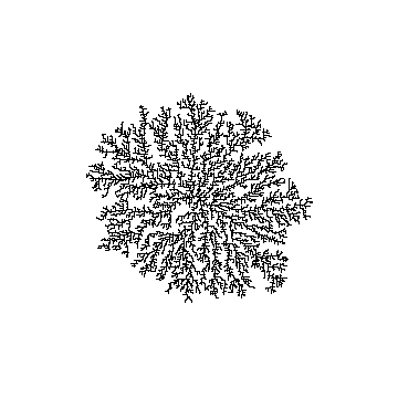
The most popular among these models is certainly diffusion-limited aggregation (DLA), suggested by Witten and Sander [21] in 1981 as a model for metal-particle aggregation. Particles arrive from ‘far away’ and perform symmetric random walks until they hit the cluster for the first time. The distribution specifying the resulting cluster formation mechanism is known as the harmonic measure. The formed clusters have a dendrite-like structure and show a fractal behaviour, see Figure 1. Another even older model is the Eden growth model due to Murray Eden [7], in which the position of the next particle is chosen uniformly out of all sites neighboring the current cluster. The clusters formed in this model tend to be very dense and appear ball like with a rough boundary. Another variation is diffusion-limited annihilation due to Meakin and Deutch [15], nowadays better known as internal DLA. Here the particles start at the origin, i.e. within the cluster, perform symmetric random walks and are attached where they exit the cluster. As in the Eden model, the formed clusters tend to be ball-like with a rough boundary.

Another popular model in the physics literature is the Vold-Sutherland model or ballistic aggregation, in which arriving particles travel along straight lines (ballistic trajectories) and stick where they hit the cluster. It can be traced back to the work of the colloid chemists Marjorie J. Vold and David N. Sutherland, see e.g. [14, 20]. It has been suggested for situations in which molecules move in a low density vapour such that thermal interactions can be disregarded. The clusters formed by this model are denser than the ones formed by DLA, but have a similar dendritic structure, see Figure 1.

All these models and many variants have been studied intensively in physics and have found numerous applications, we refer to the surveys and books [20, 19, 8, 11, 3] for further details and references. Most results have been obtained either from simulations or from intriguing but non-rigorous theoretical considerations. Some of these models have also inspired mathematical research and a number of results have been obtained. However, the progress up to now is far behind what physicists have discovered.

One of the most basic questions (to which we will mainly restrict our attention in this paper) is the speed of growth of the radius (or diameter) of the cluster as the number of particles tends to $\infty$. Regarding DLA, some rigorous almost sure bounds are due to Kesten [9, 10] (with some improvements for dimension 3 in [12] and recently in [4]), which we will recall in Section 3 below. They imply in particular that DLA clusters are not full-dimensional (in a discrete sense) and thus exhibit some fractal behaviour. For internal DLA (and the Eden model), the growth rate is $n^{1/d}$ in ${\mathbb{Z}}^{d}$, as the number of particles tends to $\infty$ and thus the clusters are full-dimensional. For internal DLA even some shape theorems have been established showing that asymptotically the clusters are balls [13]. For the Eden model the existence of a limit shape is also known, due to some relation of this model to first passage percolation, cf. [1] and the references therein. The limit shape is conjectured to deviate from a Euclidean ball. Up to now this has only been established in very high dimensions. We refer to the survey article [17] for an overview of further results regarding DLA und internal DLA. In particular, in this article, attention is also given to results obtained on graphs other than the hypercubic lattices ${\mathbb{Z}}^{d}$ that we restrict ourselves to here. (It is obvious that the models may be transferred to any infinite connected graph.) In contrast to the situation for the other mentioned models, it seems that the ballistic model has not been investigated in the maths literature so far. To the best of our knowledge, the only paper, where it is mentioned (but not analyzed very far) is the article [16], in which also a number of new aggregation models are proposed and simulated.

In this article we make a first attempt to investigate rigorously the growth behaviour of the ballistic model. To this end, we start from a more general viewpoint and set up a natural class of models (incremental aggregation), which includes the models mentioned above (and many more). We revisit the argument of Kesten that he used in [9] to obtain an upper bound on the growth rates of DLA in ${\mathbb{Z}}^{2}$ and observe that the same argument may be applied to any incremental aggregation model. In a nutshell, the ‘method’ reduces the problem of finding a bound for the radial growth to the much easier task to establish an upper bound on the local mass of the distributions determining the model. We do not claim much originality here, as once the class of incremental aggregation models is set up it is fairly easy to see that Kesten’s argument works in general. Then we apply this new method to the ballistic model. First we give a rigorous definition of the ballistic model using some notions from geometric probability. Then we state some bound on the local mass for the ballistic measures (i.e., the distributions defining the ballistic model) and finally we apply Kesten’s method to obtain the desired growth rates. It turns out that the method has power in particular in dimension $d=2$. For the ballistic model in ${\mathbb{Z}}^{2}$ we establish that the growth exponent is $1/2$ (i.e., the fractal dimension is 2), which is the value conjectured in the physics literature. For $d\geq 3$, our results imply that the fractal dimension is bounded from below by 2 (while the conjectured value is $d$).

In order to illustrate our results, we have also simulated aggregation clusters of the ballistic model (as we define it here) and DLA for comparison. The Python code is freely available, cf. [6], together more pictures of large simulated clusters.

The paper is organized as follows. In Section 2, we introduce incremental aggregation and show that this class of models includes DLA and the Eden model. In Section 3 we provide some definitions regarding radial growth and state some trivial facts about growth exponents and fractal dimensions of our models. We also recall the results of Kesten on the radial growth of DLA. In Section 4, we state Kesten’s method (Theorem 4.1) for general incremental aggregation and demonstrate how it can be applied to recover Kesten’s growth bounds for DLA and the known bounds for the Eden model. In Section 5, we define the ballistic model and apply Kesten’s method to obtain the mentioned results on the growth of these models. Finally, in Section 6 we provide a proof of our main tool, Kesten’s method.

We set up a framework in which all the models can be treated in a unified way. Let $\mathcal{P}^{d}_{f}$ denote the family of finite subsets of ${\mathbb{Z}}^{d}$, i.e.

which we equip with the discrete $\sigma$-algebra. We consider the nearest neighbor graph on ${\mathbb{Z}}^{d}$, i.e., the graph $({\mathbb{Z}}^{d},E)$ with vertex set ${\mathbb{Z}}^{d}$ and edge set $E:=\{\{x,y\}\subset{\mathbb{Z}}^{d}:\|x-y\|=1\}$. (Here and throughout $\|\cdot\|$ denotes the Euclidean norm.) A set $A\in\mathcal{P}^{d}_{f}$ is called connected, if the subgraph of $({\mathbb{Z}}^{d},E)$ generated by $A$ is. For $A\in\mathcal{P}^{d}_{f}$, the (outer) boundary of $A$ is the set

Throughout let $(\Omega,\mathcal{A},{\mathbb{P}})$ be some suitable probability space. For $A\in\mathcal{P}^{d}_{f}\setminus\{\emptyset\}$, a random point in $A$ is a measurable mapping $y_{A}:\Omega\to{\mathbb{Z}}^{d}$ with ${\mathbb{P}}(y_{A}\in A)=1$. Denote by $\mathcal{D}(A)$ the family of all probability measures on $A$, i.e., of all possible distributions of a random point in $A$. Moreover, a random finite set is a measurable mapping $F:\Omega\to\mathcal{P}^{d}_{f}$.

$F_{n}$ is called cluster or aggregate at time $n$, and $F_{\infty}:=\bigcup_{n\in{\mathbb{N}}}F_{n}$ the infinite cluster. Observe that

Moreover, for any $n\in{\mathbb{N}}$, almost surely $F_{n}$ is connected and $\#F_{n}=n$. It is easy to see that $(F_{n})_{n}$ is a Markov chain, in particular, $F_{n+1}$ depends on $F_{n}$, but not on the order, in which the points have been added to $F_{n}$. Different aggregation models arise now by choosing different families $\mathcal{M}$ of distributions. We start with the simple example of the Eden growth model.

Our second example of incremental aggregation is diffusion limited aggregation. It has been introduced by Witten and Sander [21] as a model for metal-particle aggregation and became soon very popular in physics as a simple model for many different phenomena, where particles aggregate irreversibly and diffusion (thermal motion) is the means of particle transport.

Below in Section 5 we will discuss another class of models called ballistic aggregation. In these models the particles travel along straight lines instead of random walk paths. In order to introduce them properly, we will need some concepts from geometric probability.

Our aim is to study the speed of growth of aggregation clusters in incremental aggregation models. For any finite set $A\subset{\mathbb{Z}}^{d}$ with $0\in A$, let

denote its radius, where $\|\cdot\|$ denotes the Euclidean norm. Observe that

justifying the terminology. Denote by $\operatorname{diam}(A)$ the diameter of $A$ and note that

Instead of the radius one could similarly work with the diameter in the sequel, which might be more natural in any more general setting. Since we are only interested in incremental aggregation, which is started at $0$, we stick to the radius for historic reasons. The following simple observation bounding the radius of a finite set $A\subset{\mathbb{Z}}^{d}$ in terms of its cardinality $\#A$ turns out to very useful.

Note that the constant $\frac{1}{2}$ in (3.3) could be improved but we do not need it in the sequel. Note also that for the first inequality the assumption that $A$ is connected and contains $0$ is not needed.

Let $(A_{n})_{n\in{\mathbb{N}}}$ be an increasing sequence of finite subsets of ${\mathbb{Z}}^{d}$. We are looking for a suitable exponent $\alpha$ (the ‘growth rate’ of the sequence) and a suitable constant $c>0$ such that

(Here $a_{n}\sim b_{n}$ means that the quotient $a_{n}/b_{n}$ converges to 1 as $n\to\infty$.) Since such exponent $\alpha$ might not exist in general, we define the lower and upper growth rate of the sequence $(A_{n})$ by

Alternatively, the lower and upper fractal dimension are defined by

It is immediately clear from the definitions that fractal dimension and growth rate are directly connected. In general one has $\underline{\delta}_{f}=1/\overline{\alpha}_{f}$ and $\overline{\delta}_{f}=1/\underline{\alpha}_{f}$. This means in particular that an upper bound on the growth rate implies a lower bound on the fractal dimension and vice versa.

$\#A_{n}$ may be interpreted as the volume of the cluster $A_{n}$. (We may identify $\#A_{n}$ with the union $\square A_{n}:=\bigcup_{y\in A_{n}}C_{y}$, where $C_{y}:=y+[-\frac{1}{2},\frac{1}{2}]^{d}$ is the unit cube centered at $y$. Then the volume of $\square A_{n}$ is exactly $\#A_{n}$.) Moreover, ${\rm rad}(A_{n})$ may be interpreted as the diameter, cf. (3.2), which justifies calling the exponents $\underline{\delta}_{f}$ and $\overline{\delta}_{f}$ fractal dimensions.

The trivial bounds on the radius stated in Lemma 3.1 imply immediately some general bounds on the fractal dimensions and growth rates.

In incremental aggregation models, the sequence $(F_{n})_{n\in{\mathbb{N}}}$ consists of random sets and therefore, for each $n\in{\mathbb{N}}$, ${\rm rad}(F_{n})$ is a nonnegative random variable (while $\#F_{n}=n$ is constant almost surely). Hence the fractal dimensions and growth rates are random variables, too. Observe that they satisfy almost surely the bounds stated in Proposition 3.2.

Let now $(F_{n})_{n\in{\mathbb{N}}}$ be DLA in ${\mathbb{Z}}^{d}$, $d\geq 2$ as defined in Example 2.3. The following celebrated result due to Kesten provides an almost sure upper bound on the radii of DLA clusters. For $d=3$, a log-term appears which was improved slightly by Lawler [12] and later again by Benjamini and Yadin [4].

Theorem 3.3 implies the following lower bounds on the fractal dimension.

Simulations of the model suggest that the above bounds are not sharp. In ${\mathbb{Z}}^{2}$ they suggest that the fractal dimension exists and equals $\delta_{f}=\frac{5}{3}\approx 1.66$, which is strictly larger than the rigorous bound stated above. For general $d\geq 2$, it is conjectured, cf. e.g. [20], that for DLA in ${\mathbb{Z}}^{d}$ the dimension is given by

In his paper [9], Kesten used a certain strategy of proof for his bounds for the DLA model in ${\mathbb{Z}}^{2}$, which is also described in Lawler’s book, see [12, § 2.6], and generalized to arbitrary graphs with bounded degree in [4]. It turns out that this method can be adapted to provide some bounds for any incremental aggregation model. The next theorem below describes this general method. Its proof will be discussed later in Section 6. Let $\mathcal{P}^{d}_{\partial}$ be the family of outer boundaries of aggregation clusters in ${\mathbb{Z}}^{d}$, that is, let

Recall that in any incremental aggregation model, at any time step $n$ the next point $y_{n+1}$ to be attached is chosen from the outer boundary $\partial F_{n}$ of the current cluster $F_{n}$. Therefore, it is in fact sufficient to specify the distributions $\mu_{B}$ for all $B\in\mathcal{P}^{d}_{\partial}$ in order to determine an incremental aggregation model completely. As a consequence, it is sufficient to impose conditions on the distribution family only for the distributions of outer boundary sets as in the statement below. Other sets are not relevant for the model.

The method is rather crude. Roughly it says that if for all relevant distributions in the family $\mathcal{M}$ the mass concentrated on single vertices is not too large compared to the radius of the corresponding cluster (implying that the probability mass must be spread out over a significant number of vertices), then some bound on the radial growth follows. This is plausible. The more spread out distributions are, the more options there are for the next particle to be placed. As only few of the possible locations are extremal in the sense that they lead to radial growth of the cluster, this limits the speed of growth.

In [4], the assumption (4.1) is called a $\varphi$-radius Beurling estimate in the context of the DLA model (for the function $\varphi(r)=cr^{-q}$). Our proof of Theorem 4.1 in Section 6 below follows essentially the proof of Lawler [12, § 2.6] but one might also want to compare it with [4, Lemma 2.4 and Theorem 2.6]. The important observation is that the relevant arguments in these proofs do not only apply to DLA but to any incremental aggregation.

To illustrate Kesten’s method, we briefly describe how it is applied to obtain the known bounds in ${\mathbb{Z}}^{2}$ for DLA and the Eden model. In the next section, we will use it to study ballistic aggregation. For the DLA model in ${\mathbb{Z}}^{2}$, one can use the following well known estimate for harmonic measures.

Observe that outer boundaries need not be connected such that the above estimates are not directly applicable. However, since any random walk started outside a set $A$ will first hit $\partial A$ before hitting $A$, we have

Hence the above estimates hold also for any boundary set $B\in\mathcal{P}^{d}_{\partial}$. Applying Theorem 4.1 to DLA in ${\mathbb{Z}}^{2}$, for which, by Proposition 4.2, the hypothesis is satisfied for $q=1/2$, we conclude the existence of a constant $c>0$ such that almost surely ${\rm rad}(F_{n})\leq c\,n^{3/2}$ for $n$ sufficiently large. This is the bound stated in Theorem 3.3 above.

For the Eden growth model in ${\mathbb{Z}}^{d}$ (as defined in Example 2.2 above), we have the following estimate for the defining family of distributions $(\mu_{A})$:

Applying now Kesten’s method to the Eden growth model $(F_{n})_{n}$ in ${\mathbb{Z}}^{d}$ using the estimate provided in Lemma 4.4 (for the exponent $q=1$), we infer that there is a constant $c>0$, such that almost surely

for $n$ sufficiently large. This implies $\underline{\delta}_{f}\geq 2$ for the lower fractal growth dimension of the Eden model in ${\mathbb{Z}}^{d}$. For $d=2$, by Proposition 3.2, we therefore recover

It is also well known that $\delta_{f}=d$ for the Eden model in ${\mathbb{Z}}^{d}$, $d\geq 3$, but Kesten’s method as stated in Theorem 4.1 is not capable of providing such a result, as this would require an estimate of the form (4.1) with $q=d-1$, which is simply not true. Indeed, for any $r\in{\mathbb{N}}$ there is a cluster $A$ such that for $B=\partial A$, ${\rm rad}(B)=r$ and $\mu_{B}(z)\geq(2(d-1))^{-1}r^{-1}$. (Take e.g. $A:=\{(k,0,\ldots,0)\in{\mathbb{Z}}^{d}:k\in\{0,1,\ldots,r-1\}$. Then $\#B=2+2(d-1)r\leq 2(d-1)r$ and so $\mu_{B}(z)\geq(2(d-1))^{-1}r^{-1}$.) This precludes an estimate of the form (4.1) to hold for any $q>1$.

The hypothesis in Kesten’s method is rather restrictive. Requiring some deterministic estimate to be satisfied for all outer boundaries and at all locations $z$ leads to an exponent $q$ that is often too small in order to provide a good bound for the radial growth. Although the methods is able to provide lower bounds on radial growth in any dimension $d$, it seems that the method is strong only in ${\mathbb{Z}}^{2}$.

It seems plausible, that it should be enough to have a bound on $\mu_{\partial A}(z)$ available for outer boundaries of ’typical’ aggregation clusters $A$ (or for ’most of them’). However, this will require further investigation and is not covered by Theorem 4.1 above. Another approach (which leads in fact to the growth bounds for DLA stated above) are estimates in terms of the volume of the clusters rather than its radius, which will be a topic of further investigation.

We now introduce the ballistic model rigorously and discuss its growth properties. Ballistic aggregation in ${\mathbb{Z}}^{d}$ will be defined as incremental aggregation $(F_{n})_{n\in{\mathbb{N}}}$ with a suitable distribution family $\mathcal{M}=(b_{A})_{A\in\mathcal{P}^{d}_{f}}$. In order to determine the model all we have to do is to choose the family $\mathcal{M}$, i.e., to fix a distribution $b_{A}$ on each finite set $A\in\mathcal{P}^{d}_{f}$. Roughly, for each $z\in A$, $b_{A}(z)$ will be determined by the probability that a ‘directed random line through $A$ hits $z$ first’. In order to define this properly, we recall some ideas from stochastic geometry, in particular the concept of an isotropic random line. In what follows, we will view ${\mathbb{Z}}^{d}$ also as a subset of ${\mathbb{R}}^{d}$ embedded in the natural way.

Let $A(d,1)$ be the space of lines in ${\mathbb{R}}^{d}$ (i.e., the affine Grassmannian of $1$-flats). We equip it with the usual hit-or-miss topology and the associated Borel $\sigma$-algebra $\mathcal{A}(d,1)$, see e.g. [18, Chapter 13] for details. For any compact set $K\subset{\mathbb{R}}^{d}$ let

Then $\mathcal{A}(d,1)=\sigma(\{[K]:K\in\mathcal{K}^{d}\})$, where $\mathcal{K}^{d}$ denotes the family of all convex bodies, that is, compact, convex sets in ${\mathbb{R}}^{d}$.

It is well known, cf.  e.g. [18], that there is a unique Euclidean motion-invariant Radon measure $\mu_{1}$ on $A(d,1)$ such that

Here $B_{n}$ is the unit ball in ${\mathbb{R}}^{n}$ and $\kappa_{n}:=\lambda_{n}(B_{n})$ denotes its volume.

Observe that, by the Crofton formula, cf. e.g. [18, Theorem 5.1.1], for any convex body $K\in\mathcal{K}^{d}$,

where the constant is given by $\alpha_{d}:=\frac{2(d-1)!\kappa_{d-1}}{d!\kappa_{d}}=\frac{2\kappa_{d-1}}{d\kappa_{d}}$ and $V_{j}(K)$ is the intrinsic volume of $K$ of degree $j$. If $K$ has nonempty interior, then $V_{d-1}(K)$ is half the surface area of $K$. This means, the measure of lines hitting a given convex body $K$ is up to some universal constant given by the surface area of $K$. Following [18, Definition 8.4.2], for any convex body $K\in\mathcal{K}^{d}$ with $V_{d-1}(K)>0$, an isotropic random line through $K$ is defined to be a random variable $L:\Omega\to A(d,1)$ with distribution given by

This definition extends without any problem to arbitrary compact sets $K\subset{\mathbb{R}}^{d}$, provided that $\mu_{1}([K])>0$. However, the convenient interpretation (5.1) of $\mu_{1}$ in terms of $V_{d-1}$ (or the surface area) is no longer valid if $K$ is not convex. Observe that for any compact $K\subset{\mathbb{R}}^{d}$, one has $\mu_{1}([K])\leq\mu_{1}\left(\left[\operatorname{conv}(K)\right]\right)<\infty$, where $\operatorname{conv}(K)$ denotes the convex hull of $K$. Thus, for any compact set $K\subset{\mathbb{R}}^{d}$ with $\mu_{1}([K])>0$, the distribution ${\mathbb{P}}^{K}$ is well defined and so is an isotropic random line through $K$. In ${\mathbb{R}}^{2}$ one has the following additional property, which turns out to simplify the analysis significantly: for any connected, compact set $C\subset{\mathbb{R}}^{2}$,

Therefore, ${\mathbb{P}}^{C}={\mathbb{P}}^{\operatorname{conv}(C)}$ (provided $V_{1}(\operatorname{conv}(C))>0$, i.e., $C$ not a singleton). Thus in dimension 2 one can work with convex hulls instead of the original sets. Unfortunately, this is not possible in any higher dimension.

For any finite set $A\in\mathcal{P}^{d}_{f}$ denote by $\square A$ the union of grid boxes centered in $A$, that is, let

Then, for any $d\geq 2$ and $A\in\mathcal{P}^{d}_{f}\setminus\{\emptyset\}$, the distribution ${\mathbb{P}}^{\square A}$ of an isotropic random line through $\square A$ is well defined. The idea for the definition of the ballistic measure $b_{A}$ is now as follows: We identify $A$ with $\square A$ and generate an isotropic random line $L$ through $\square A$. We choose randomly a direction on $L$. Then for any $z\in A$, we let $\mu_{A}(z)$ be the probability that, when traveling along $L$ in the chosen direction, the square $C_{z}$ is the first square in $\square A$ visited by $L$. More formally, we fix for each $L\in A(d,1)$ a direction $v_{L}\in\mathbb{S}^{d-1}$. (We choose $v_{L}$ such that the mapping $L\mapsto v_{L}$ is measurable.) For $A\in\mathcal{P}^{d}_{f}$ and $L\in A(d,1)$, let

that is, $L^{A}$ is the set of those points in $A$ whose associated boxes are intersected by $L$. Traversing $L$ in direction $v_{L}$ induces an order in $L^{A}$. (For certain lines the order in which the boxes are visited is not well defined, namely if $L$ hits a box first at an intersection point of two or several boxes not visited before. In such a case the order can be made unique by fixing some order of the boxes $C_{z}$ in $z\in{\mathbb{Z}}^{d}$, such as the one induced by the lexicographic order in ${\mathbb{Z}}^{d}$. However, for $\mu_{1}$-almost all lines $L$ the order in $L^{A}$ is well defined without this.) Denote by $\min(L^{A})$ and $\max(L^{A})$ the first and last point in $L^{A}$ ‘visited’ by $L$.

Observe that $b_{A}(z)=0$ for $z\notin A$ and $\sum_{z\in A}b_{A}(z)=1$. Hence, $b_{A}$ is indeed a probability measure which is concentrated on $A$, that is, $b_{A}\in\mathcal{D}(A)$. Note also that, for any $z\in A$,

This gives a first upper bound of the probability mass of $b_{A}$ at single vertices. Ballistic aggregation (BA) on ${\mathbb{Z}}^{d}$ is now defined to be incremental aggregation with distribution family $(b_{A})_{A\in\mathcal{P}^{d}_{f}}$, where $b_{A}$ is the ballistic measure on $A$.

For the ballistic model in ${\mathbb{Z}}^{d}$, $d\geq 2$, we have the following main result concerning the radial growth of clusters, which parallels the one obtained by Kesten for DLA.

Combining this bound with the trivial lower bound provided by Propositon 3.2, we conclude that in ${\mathbb{Z}}^{2}$ the fractal dimension $\delta_{f}$ of BA clusters exists and equals $2$. This confirms a long standing conjecture in the physics literature, cf. [5, 14, 2, 20].

For $d\geq 3$, the conclusion regarding the fractal dimension of the BA model is not quite as strong as for $d=2$.

As in the case $d=2$, this can be directly deduced from Theorem 5.2. Unfortunately, this lower bound for the fractal dimension is far from the conjectured value $\delta_{f}=d$ in this case.

The proof of Theorem 5.2 will be based on Kesten’s method (Theorem 4.1 above). In order to apply it, a suitable estimate for the local growth of the ballistic measures $b_{A}$ is required, which we state now.

Before we provide a proof of Proposition 5.6, we first clarify that Theorem 5.2 easily follows from this statement.

Observe that any improvement on the exponent $q=1$ in Proposition 5.6 (i.e., any larger $q$) would allow to deduce from Kesten’s method a better bound for the radial growth. Unfortunately, the exponent $q=1$ in Proposition 5.6 turns out to be optimal in any dimension $d\geq 2$, as the following remark clarifies.

References

- [1] A. Auffinger, M. Damron, and J. Hanson. 50 years of first-passage percolation, volume 68 of University Lecture Series. American Mathematical Society, Providence, RI, 2017. doi:10.1090/ulect/068.
- [2] R. C. Ball and T. A. Witten. Causality bound on the density of aggregates. Phys. Rev. A, 29:2966–2967, May 1984. URL: https://link.aps.org/doi/10.1103/PhysRevA.29.2966, doi:10.1103/PhysRevA.29.2966.
- [3] A.-L. Barabási and H. E. Stanley. Fractal Concepts in Surface Growth. Cambridge University Press, 1995. doi:10.1017/CBO9780511599798.
- [4] I. Benjamini and A. Yadin. Upper bounds on the growth rate of diffusion limited aggregation, 2017. arXiv:1705.06095.
- [5] D. Bensimon, E. Domany, and A. Aharony. Crossover of fractal dimension in diffusion-limited aggregates. Phys. Rev. Lett., 51:1394–1394, Oct 1983. URL: https://link.aps.org/doi/10.1103/PhysRevLett.51.1394, doi:10.1103/PhysRevLett.51.1394.
- [6] T. Bosch. Incremental-aggregations. https://github.com/tillmanntristanbosch/incremental-aggregations, 2021. Accessed: 2023-08-23.
- [7] M. Eden. A two-dimensional growth process. In Proc. 4th Berkeley Sympos. Math. Statist. and Prob., Vol. IV, pages 223–239. Univ. California Press, Berkeley, Calif., 1961.
- [8] R. Jullien and R. Botet. Aggregation and fractal aggregates. World Scientific Publishing Co., Inc., Teaneck, NJ, 1987.
- [9] H. Kesten. How long are the arms in DLA? J. Phys. A, 20(1):L29–L33, 1987. doi:10.1088/0305-4470/20/1/007.
- [10] H. Kesten. Upper bounds for the growth rate of DLA. Phys. A, 168(1):529–535, 1990. doi:10.1016/0378-4371(90)90405-H.
- [11] M. Kolb. Structure Formation by Aggregation: Models and Applications, pages 381–389. Springer Berlin Heidelberg, Berlin, Heidelberg, 2001. doi:10.1007/3-540-44946-9_31.
- [12] G. F. Lawler. Intersections of random walks. Probability and its Applications. Birkhäuser Boston, Inc., Boston, MA, 1991.
- [13] G. F. Lawler, M. Bramson, and D. Griffeath. Internal diffusion limited aggregation. Ann. Probab., 20(4):2117–2140, 1992. URL: http://links.jstor.org/sici?sici=0091-1798(199210)20:4<2117:IDLA>2.0.CO;2-K&origin=MSN.
- [14] P. Meakin. The Vold-Sutherland and Eden models of cluster formation. Journal of Colloid and Interface Science, 96(2):415–424, 1983. URL: https://www.sciencedirect.com/science/article/pii/0021979783900449, doi:10.1016/0021-9797(83)90044-9.
- [15] P. Meakin and J. M. Deutch. The formation of surfaces by diffusion limited annihilation. The Journal of Chemical Physics, 85(4):2320–2325, 08 1986. arXiv:https://pubs.aip.org/aip/jcp/article-pdf/85/4/2320/11207514/2320\_1\_online.pdf, doi:10.1063/1.451129.
- [16] I. S. Molchanov. Diffusion-limited aggregation with jumps and flights. J. Statist. Comput. Simulation, 64(4):357–381, 1999. doi:10.1080/00949659908811985.
- [17] E. Sava-Huss. From fractals in external DLA to internal DLA on fractals. In Fractal Geometry and Stochastics VI, volume 76 of Progr. Probab., pages 273–298. Birkhäuser/Springer, 2021. URL: https://doi.org/10.1007/978-3-030-59649-1_12, doi:10.1007/978-3-030-59649-1\_12.
- [18] R. Schneider and W. Weil. Stochastic and integral geometry. Probability and its Applications (New York). Springer-Verlag, Berlin, 2008. doi:10.1007/978-3-540-78859-1.
- [19] H. E. Stanley and N. Ostrowsky, editors. On growth and form, volume 100 of NATO Advanced Science Institutes Series E: Applied Sciences. Martinus Nijhoff Publishers, Dordrecht, 1986. Fractal and nonfractal patterns in physics, Papers from a course given as part of the NATO-ASI series at the Cargèse summer school, Cargèse, June 26–July 6, 1985.
- [20] T. Vicsek. Fractal growth phenomena. World Scientific Publishing Co., Inc., Teaneck, NJ, 1989. With a foreword by Benoit B. Mandelbrot. doi:10.1142/0511.
- [21] T. A. Witten and L. M. Sander. Diffusion-limited aggregation, a kinetic critical phenomenon. Phys. Rev. Lett., 47:1400–1403, Nov 1981. URL: https://link.aps.org/doi/10.1103/PhysRevLett.47.1400, doi:10.1103/PhysRevLett.47.1400.