On the Potential Function of the Colored Jones Polynomial and the AJ conjecture
Abstract.
The -polynomial is conjectured to be obtained from the potential function of the colored Jones polynomial by elimination. The AJ conjecture also implies the relationship between the -polynomial and the colored Jones polynomial. In this paper, we connect these conjectures from the perspective of the parametrized potential function.
Key words and phrases:
potential function, the volume conjecture, the AJ conjecture.2020 Mathematics Subject Classification:
57K14, 57K31, 57K321. Introduction
Quantum invariants closely relate to the -dimensional geometry. One of the crucial conjectures is the volume conjecture.
Conjecture 1.1 (Volume Conjecture [9]).
For any knot , the colored Jones polynomial satisfies
where is the volume of the ideal regular tetrahedron in the three-dimensional hyperbolic space and is the simplicial volume for the complement of .
Yokota [14] considered the potential function of the Kashaev invariant and established a relationship between a saddle point equation and a triangulation of a knot complement. We also considered the potential function of the colored Jones polynomial with parameters corresponding to the colors and found a geometric meaning of derivatives with those parameters in [11]. In the knot case, the upshot is as follows: Let be a hyperbolic knot, and let be a potential function of the colored Jones polynomial for evaluated at the root of unity. Here, corresponds to the half of the color. Then,
| ( 1.1) |
is the condition that the knot complement admits a hyperbolic structure. Here, is the dilation component of the preferred longitude. In this connection, the -polynomial is conjectured to be obtained from such a parametrized potential function by elimination [6, 15].
On the other hand, the AJ conjecture, which states that the -polynomial is obtained by the recurrence of the colored Jones polynomial, is known as a relationship between the colored Jones polynomial and the -polynomial.
Conjecture 3.1 (the AJ conjecture [3]).
For any knot , is equal to up to multiplication by an element in , where is an evaluation map at .
Garoufalidis [3] proposed this conjecture, and Takata [12], for example, observed it with twist knots. Detcherry and Garoufalidis [2] also considered the AJ conjecture from the perspective of a triangulation of the knot complement.
In this paper, we connect these conjectures on the relationship between the colored Jones polynomial and the -polynomial via the potential function. The -polynomial is obtained from the summand of the colored Jones polynomial by creative telescoping (See [3, 4] or Section 3). We will compare this process with the above conjectural method to obtain the -polynomial. For an odd number , let be a summand of the colored Jones polynomial for a knot , where is an integer satisfying . Since is restricted to odd numbers, the following discussion is on the -invariants. Let , and be shift operators, and let be an evaluation map at . Then, we verify the following proposition:
The background of Proposition 4.1 is that the ratio of summands is approximated by a potential function for sufficiently large integers . For example,
See Remark 4.2 for details. From these facts, we would like to propose the conjecture that the factor of the polynomial for a knot corresponding to the inhomogeneous recursive relation yields the factor of the -polynomial for the knot corresponding to nonabelian representaitions.
Conjecture 4.3.
equals up to multiplication by an element in , where
Here, the polynomial is called the nonabelian -polynomial [8].
This paper is organized as follows: In Section 2, we review the potential function, the -polynomial, and their conjectural relationship. In Section 3, we briefly look over the -polynomial and creative telescoping. In Section 4, we compare those themes and verify the above proposition.
Acknowledgments. The author is grateful to Jun Murakami and Seokbeom Yoon for their helpful comments.
2. Potential Functions and -polynomials
2.1. -polynomial
In this subsection, we review the difinition of the -polynomial following [1]. Let be a knot, and let be its complement. The set of all -representations is an affine algebraic variety. Then, we restrict our attention to
where is the meridian, and is the preferred longitude of . We can define the eigenvalue map by , where
For an algebraic component of , the Zariski closure of is an algebraic subset of . If is a curve, there exists a defining polynomial. The -polynomial of a knot is the product of all such defining polynomials.
2.2. Potential functions
On the other hand, we provided the geometric meaning of derivatives of a potential function of the colored Jones polynomial. Let us recall some facts on the potential function briefly. See [11, 16] for details.
Definition 2.1.
Suppose that the asymptotic behavior of a certain quantity for a sufficiently large is
where grows at most polynomially and is a region in . We call this function a potential function of .
The potential function of the colored Jones polynomial evaluated at the root of unity is obtained by approximating -matrices with continuous functions. Let and be odd numbers. The summands of the -matrix of the colored Jones polynomial that is assigned to a crossing are as follows [11]:
| ( 2.1) | ||||
| ( 2.2) | ||||
Here, and are integers satisfying and , is an indeterminate, and . We also note that we assign to a positive crossing, and to a negative crossing. On the other hand, corresponding potential functions are as follows:
Here, is the dilogarithm function, corresponds to , corresponds to , and , with , corresponds to , where is an integer, and is the -th root of unity . These indices or parameters are labeled to regions of a link diagram. A potential function of the colored Jones polynomial for a -component hyperbolic link evaluated at is the summation of . Here, is a -tuple of the parameters corresponding to the colors, and is a signature of the crossing , and runs over all crossings. This potential function essentially coincides with the generalized potential function in [16]111In [16], Yoon defined the generalized potential function and established the relationship between the gluing equation. The author appreciates Yoon’s valuable comment at the 18th East Asian Conference on Geometric Topology.. We will review some facts on the potential function. From the saddle point of the potential function , we can obtain a hyperbolic structure of the complement of the link that is not necessarily complete. This is because
coincides with the gluing equation of an ideal triangulation of . Here, we choose the saddle point so that the imagaginary part of the potential function satisfies
where is the hyperbolic volume of the link . Then, the following equality holds:
where is the dilation component of the action of the preferred longitude of the link component . In other words, if
has a solution, then has a corresponding hyperbolic structure. Since each equation is equivalent to a polynomial equation, we can determine the condition of whether the system of the equations has a solution by elimination. In fact, the -polynomial is conjectured to be obtained by the potential function of the colored Jones polynomial [6, 15].
3. -polynomial and AJ conjecture
3.1. -polynomial
For a knot , its colored Jones polynomial has a nontrivial linear recurrence relation [4]
| ( 3.1) |
where is an polynomial with integer coefficients. For a discrete function , we define operators and by
Then, we can restate the recurrence relation (3.1) as
This polynomial is an element in the non-commutative algebra
To define the -polynomial, we have to localize the algebra . Let be the automorphism of the field given by
The Ore algebra is defined by
where the multiplication of monomials is given by . The -polynomial is a generator of the recursion ideal of
with the following properties:
-
•
has the smallest -degree and lies in .
-
•
is of the form , where are coprime.
Garoufalidis proposed the following conjecture on the -polynomial:
Conjecture 3.1 (the AJ conjecture [3]).
For any knot , is equal to up to multiplication by an element in , where is an evaluation map at .
3.2. Computation of -polynomial
Definition 3.2.
For a discrete function
we define operators , , and by
These operators generate the algebra
with relations
where , and for . Hereafter, we put .
Definition 3.3.
A discrete function is called -hypergeometric if holds for all .
We especially deal with a proper -hypergeometric function.
Definition 3.4.
A -hypergeometric discrete function is called proper if it is of the form
where , are integers, are vectors of integers, are variables, is a quadratic form, is an vector of elements in , and
Proper -hypergeometric functions satisfy the following theorem:
Theorem 3.5 ([13]).
Every proper -hypergeometric function has a -free recurrence
where is a -tuple of integers, and is a finite set.
We put
| ( 3.2) |
where . The expansion of around , with , is
where , and is a polynomial in . Here, . Putting , we have
Summing up this equality, we verify that satisfies
where and are fixed parameters. Since is a proper -hypergeometric function, is a sum of proper -hypergeometric functions. That means is a sum of multisums of proper -hypergeometric functions with one variable less. Repeating this process, we obtain a polynomial such that
3.3. -polynomial and eliminations
The annihilating polynomial (3.2) of the summand is an element in . Moreover, defining the polynomials , and by
it is known that the annihilating ideal of is generated by
Therefore, we would be able to obtain an annihilating poynomial of by eliminating from
From the observation above, we would also be able to obtain by eliminating from
4. Comparison with the saddle point equation
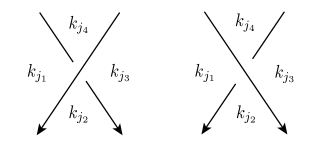
In this section, we compare the saddle point equation of the potential function of the colored Jones polynomial for a knot. First of all, we recall the -matrices of the -colored Jones polynomial associated with a crossing :
Here, is an integer satisfying , are modifications with Reidemeister move I, and the indices , with , are labeled to each region around the crossing as shown in Figure 4.1 [7, 11].
Corresponding potential functions are
Derivatives of are
| ( 4.1) | ||||
and
| ( 4.2) |
On the other hand, we have
| ( 4.3) | ||||
| ( 4.4) | ||||
| ( 4.5) | ||||
| ( 4.6) |
Furthermore, defining an operator by , we have
| ( 4.7) |
Putting we have
| ( 4.8) | ||||
and
| ( 4.9) | ||||
(4.1) and (4.2) coincide with (4.8) and (4.9) under the correspondences and . A similar argument holds for a negative crossing. We define the discrete function by
and polynomials and with , by
The equation under the substitution , which means , is equivalent to
and this corresponds to
under and . Let be an operator such that . By the definition, holds. We also define polynomials and by
Then,
holds. The equation is equivalent to
and this corresponds to
Note that the system of equations
yields an annihilating polynomial of the summand, but we can obtain an annihilating polynomial by . Note also that corresponds to the eigenvalue of the meridian. This explains the substitution of for the -polynomial in the statement of the AJ conjecture. When all indices vanish after finite times of creative telescoping, we obtain an inhomogeneous recurrence relation
| ( 4.10) |
where , and . Since can be canceled by left multiplication of , we obtain homogeneous recurrence relation
This would support the AJ conjecture. The crucial point of the above argument is as follows:
Proposition 4.1.
The system of equations
coincides with
under the correspondence .
Remark 4.2.
We can view Proposition 4.1 as follows: The potential function is obtained from the summand of the colored Jones polynomial by approximating it with continuous functions. Therefore, for a sufficiently large integer ,
Then,
By Proposition 4.1, we would be able to obtain the factor of the -polynomial for corresponding to nonabelian representations from .
Conjecture 4.3.
equals up to multiplication by an element in , where
Remark 4.4.
The polynomial is called the nonabelian -polynomial [8].
Then, the factor that annihilates in (4.10) would correspond to the factor of corresponding to abelian representations. These conjectural correspondences are illustrated in Figure 4.2.

Appendix A Example calculation for the figure-eight knot
Let us observe the process above with the figure-eight knot. The colored Jones polynomial for the figure-eight knot is [5]
where
Note that this formula is not the form itself obtained from the -matrix. The argument above, however, is still valid.
A.1. Potential function and the -polynomial
The potential function of is (see [11])
The derivatives of with and are
Noting that if is of the form
the action of is , especially its dilation component is equal to , we put
From
we obtain the factor of the A-polynomial of the figure-eight knot
| ( A.1) |
by elimination of .
A.2. Annihilating polynomials of
The annihilating polynomial of is [3]
We can factorize this polynomial as , where is
and are
| ( A.2) | ||||
Substituting and into (A.2), we have
| ( A.3) | |||
| ( A.4) |
From (A.3), we have
| ( A.5) |
Multiplying (A.4) by from the left, we obtain
| ( A.6) |
Then, we multiply (A.6) by
from the left. This polynomial is factorized in two ways.
Then, using (A.3) and (A.5), we obtain the annihilating polynomial of
The expansion of at is
where
| ( A.7) |
and
Therefore, is of the form
where , with . Summing up this equality with running from to , we have
Note that when . Putting , on the other hand, we have
Therefore, we have the second order inhomogeneous recurrence relation [3]
Since is annihilated by
we have the third order homogeneous recurrence relation .
A.3. Comparison of the derivatives and the -differences
Substituting into (A.3) and (A.4), we have
| ( A.8) | |||
| ( A.9) |
Here, the factor in (A.8) is canceled and we have
| ( A.10) |
Eliminating from (A.9) and (A.10), we obtain
| ( A.11) |
which is equal to the polynomial (A.1) under the substitutions and . The polynomial (A.11) is also equal to the one (A.7) with evaluated at
up to multiplication by an element in .
References
- [1] D. Cooper, D.D. Long, Remarks on the -polynomial of a knot. J. Knot Theory Ramifications 5, (1996), 609-628.
- [2] R. Detcherry, S. Garoufalidis, A diagrammatic approach to the AJ conjecture. Math. Ann. 378, (2020), 447-484.
- [3] S. Garoufalidis, On the characteristic and deformation varieties of a knot. Geom. Topol. Monogr. 7, (2004), 291-309.
- [4] S. Garoufalidis, T.T.Q. Lê, The colored Jones function is -holonomic. Geom. Topol. 9, (2005), 1253-1293.
- [5] K. Habiro, On the colored Jones polynomials of some simple links. Sūrikaisekikenkyūsho Kōkyūroku 1172 (2000), 34-43.
- [6] K. Hikami, Asymptotics of the colored Jones polynomial and the A-polynomial. Nucl. Phys. B 773 (2007), 184-202.
- [7] R. Kirby, P. Melvin, The 3-manifold invariants of Witten and Reshetikhin-Turaev for . Invent. Math. 105 (1991), 473-545
- [8] T.T.Q. Lê, X. Zhang, Character varieties, -polynomials and the AJ conjecture. Algebr. Geom. Topol. 17, (2017), 157-188.
- [9] H. Murakami, J. Murakami, The colored Jones polynomials and the simplicial volume of a knot. Acta Math. 186, (2001), 85-104.
- [10] J. Murakami, Colored Alexander invariants and cone-manifolds. Osaka J. Math. 45 (2008), 541-564.
- [11] S. Sawabe, On the potential function of the colored Jones polynomial with arbitrary colors. Pacific J. Math. 322, (2023), 171-194.
- [12] T. Takata, The colored Jones polynomial and the A-polynomial for twist knots. arXiv:math/0401068
- [13] H.S. Wilf, D. Zeilberger, An algorithmic proof theory for hypergeometric (ordinary and “”) multisum/integral identites, Invent. Math. 108, (1992), 575-633.
- [14] Y. Yokota, On the volume conjecture for hyperbolic knots. arXiv:math/0009165 (2000).
- [15] Y. Yokota, From the Jones polynomial to the -Polynomial of hyperbolic knots. Interdiscip. Inform. Sci. 9, (2003), 11-21.
- [16] S. Yoon, On the potential functions for a link diagram. J. Knot Theory Ramifications 30(07) (2021) 2150056 (24 pages)