On the possibility of Baryon Acoustic Oscillation measurements at redshift with the Roman Space Telescope
Abstract
The Nancy Grace Roman Space Telescope (RST), with its field of view and high sensitivity will make surveys of cosmological large-scale structure possible at high redshifts. We investigate the possibility of detecting Baryon Acoustic Oscillations (BAO) at redshifts for use as a standard ruler. We use data from the hydrodynamic simulation BlueTides in conjunction with the gigaparsec-scale Outer Rim simulation and a model for patchy reionization to create mock RST High Latitude Survey grism data for Lyman- emission line selected galaxies at redshifts to , covering 2280 square degrees. We measure the monopoles of galaxies in the mock catalogues and fit the BAO features. We find that for a line flux of , the detection limit for the current design, the BAO feature is partially detectable (measured in three out of four survey quadrants analysed independently). The resulting root mean square error on the angular diameter distance to is 7.9. If we improve the detection sensitivity by a factor of two (i.e. ), the distance error reduces to . We caution that many more factors are yet to be modelled, including dust obscuration, the damping wing due to the intergalactic medium, and low redshift interlopers. If these issues do not strongly affect the results, or different observational techniques (such as use of multiple lines) can mitigate them, RST or similar instruments may be able to constrain the angular diameter distance to the high redshift Universe.
keywords:
Cosmology: dark energy - Cosmology: large scale structure of Universe - Galaxies: statistics.1 Introduction
Baryon Acoustic Oscillations (BAO) have become very useful as a standard ruler to constrain cosmological models (see e.g., the review by Weinberg et al. (2013)). Due to the distinctive nature of their signature, the BAO scale constitutes one of the most effective observables in cosmology. The BAO features can be detected as peaks in two point correlation functions or wiggles in power spectra. These signatures of BAO can be used to measure the Hubble constant and the angular diameter distance as function of redshift. As such, it is used as a robust and unique probe to investigate the nature of dark energy.
The sound horizon at the time of recombination leaves its imprint on both the cosmic microwave background (CMB) and three dimensional distribution of matter. Using simulations, in this paper we explore whether it may be possible to measure the BAO scale at redshifts using galaxies detected by the RST satellite (formerly the Wide Field Infrared Survey Telescope, WFIRST111 https://wfirst.gsfc.nasa.gov/ ). These measurements would represent the first BAO detection between and .
The first observations made of BAO (Eisenstein et al., 2005; Cole et al., 2005)) at low redshifts () used luminous red galaxies (LRGs) as tracers of structure, and these have been supplemented by even larger samples at higher redshifts (e.g., Zhai et al. (2017), Bautista et al. (2018)), up to . The density field at redshifts is accessible using the Lyman- forest of absorption in quasar spectra, and its measured clustering has led to the determination of the BAO scale at (Busca et al., 2013; Slosar et al., 2013; du Mas des Bourboux et al., 2017; de Sainte Agathe et al., 2019). The gap between low redshift galaxy determinations and the forest was recently filled by a determination using quasar clustering at (Ata et al., 2018). Emission line galaxies at (Raichoor et al., 2017) and (Comparat et al., 2016) from the Extended Baryon Oscillation Spectroscopic Survey (eBOSS) will also soon be adding constraints in this crucial redshift range, around the time that the Universe started to accelerate. Radio observations of 21cm emission will increase the volume covered (Vanderlinde & Chime Collaboration, 2014). At higher redshifts, galaxies have been discovered as far away as (Oesch et al., 2016), in small Hubble Space Telescope (HST) fields at present. The RST satellite1 will have a much wider field of view than HST, and the planned RST grism survey holds the promise of measuring the large-scale structure of the Universe at early times with galaxy survey techniques which have been hitherto been confined to low redshifts.
Among the reasons for looking at the BAO scale in a different redshift regime are the possibility of early dark energy (Hill & Baxter, 2018), or models where dark matter decays into radiation and affects the expansion rate (Wang et al., 2014). There is also current tension between locally determined measurements (Riess et al., 2018) and those determined from the CMB in the context of cold dark matter (CDM) (Planck Collaboration et al., 2018a). Using multiple redshifts to determine the consistency (or not) of BAO measurements should be useful in finding a solution to this controversy.
Cosmological surveys designed to measure the BAO feature must cover large volumes, as the comoving length scale involved is 150 megaparsecs, and cosmic variance must be suppressed. The number density of sampling objects must be large enough to overcome shot noise. When there is domination by shot-noise, one can still obtain BAO measurements and the error will just scale as , where is the number of objects. For example, eBOSS quasars are shot-noise dominated (Zarrouk et al., 2018). The shot-noise dominated regime carries the implication that one can return to the same volume and sample it further to obtain more precise results. Conversely, when one is cosmic variance limited, one gains more from sampling a new volume instead of sampling the same volume.
The current number density of quasars at in the largest survey (final SDSS-III BOSS DR09; Eftekharzadeh et al., 2015) is (Mpc)3, which is too low. Galaxies at similar redshifts and higher exist in sufficient numbers, but their relatively low luminosity has made gathering samples that cover sufficient volume impossible with current technology. RST and Euclid will enable the Universe at to be studied with a more representative sample of galaxies than have been possible at present (small current fields of view lead to rarer brighter galaxies being missed). So far, galaxies have been found up to redshifts with dropout techniques (Ellis et al., 2013). The largest samples with photometric redshifts at are Chaikin et al. (2018), Yan et al. (2011), Bouwens et al. (2011), Laporte et al. (2017), Eyles et al. (2005) and Mobasher et al. (2005) which contain 72, 20, 1, 1, 2 and 1 galaxies respectively. In a few cases spectral confirmation has been obtained by identifiying the Lyman- line (refs for galaxies (Finkelstein et al., 2013; Song et al., 2016). Between and , the Candels survey (Pentericci et al., 2018) has found 260 spectroscopically confirmed galaxies. Narrow band imaging surveys searching directly for the Lyman- line offer a route to large samples in principle. An early example of such a search includes Tilvi et al. (2010) at which was not able to confirm any objects. More recently, the LAGER survey (Hu et al., 2017) has followed up candidates with further spectroscopy and found a 66% success rate at .
There are number of obstacles to the finding and use of galaxies as a BAO probe. The most important is the actual visibility of lines that would enable spectroscopic identification. The Lyman- line is subject to multiple scatterings and absorption by dust within galaxies. It is also absorbed by neutral hydrogen content of the intergalactic medium (IGM), and Lyman- emitting galaxies at the highest redshifts have proved difficult to find. One the other hand, at , Bagley et al. (2017) have found that Lyman- emitters are detectable and may lie mainly in ionized bubbles, sufficiently large for the Lyman- photons to redshift out of resonance before encountering the neutral IGM gas. At lower redshifts (e.g., ), Lyman- emission appears to have an escape fraction of % (Gronwall et al., 2007; Francis et al., 2012) but at higher redshifts it appears to climb to near 100% (Cassata, P. et al., 2011; Sobacchi & Mesinger, 2015).
Interlopers are another important issue. For example there will be galaxies at redshifts for which Hydrogen Balmer lines will fall in the spectral window for Lyman- at redshifts . Intermediate redshift () galaxies will also contribute [OIII] 5007 emission. How well RST grism spectra could be used to identify galaxies at the highest redshifts and remove interlopers is an open question.
In this paper we carry out the simplest analysis possible, using a combination of a large darkmatter simulation (Outer Rim; Li et al., 2019) and a hydrodynamic simulation (BlueTides; Wilkins et al., 2016a; Wilkins et al., 2016b) to see whether BAO could be detected at redshifts with RST’s spectral coverage. We make many simplifying assumptions, each of which are likely to strongly affect the outcome, but can be tested with future work. We assume that all Lyman- emission can be seen. In other words, we suppose that the Lyman- emitting galaxies lie in ionized bubbles (Kakiichi et al., 2016; Yajima et al., 2018). We ignore galaxy-scale extinction of Lyman- emission. That is, we assume that the raw star formation in our hydrodynamic simulation of galaxy formation, BlueTides (Wilkins et al., 2016a; Wilkins et al., 2016b) can be directly translated into Lyman- luminosity. We also do not directly address interlopers and do not do a complete analysis of spectral overlap in the grism spectra. We restrict ourselves to seeing whether mock observations of a RST grism survey under these conditions can detect the BAO feature. Our analysis therefore acts as a first step - if we find that it is possible, then these restrictions should be relaxed and tested to see whether it is worth pursuing the idea further.
The plan for the paper is as follows. In Section 2 we describe the different cosmological datasets we use. In Section 3 we show how these were used to construct mock catalogues for the RST high latitude survey. We describe details results obtained from mock catalogues in Section 4. We present comprehensive discussion and analysis of our results in Section 5.
| Name | BlueTides | Outer Rim | |
|---|---|---|---|
| 0.7186 | 0.7352 | ||
| 0.2814 | 0.2648 | ||
| 0.0464 | 0.04479 | ||
| h | 0.697 | 0.71 | |
| 0.820 | 0.8 | ||
| 0.971 | 0.963 |
2 Datasets
2.1 The BlueTides simulation
BlueTides is a hydrodynamic simulation which was designed to cover the high redshift Universe (Feng et al., 2015, 2016). The model uses the Smoothed Particle Hydrodynamics code MP-Gadget to evolve a cubical volume with particles. These particles are used to model dark matter, gas, stars and supermassive black holes. This simulation evolved a cMpc3 cube to redshift . The resolution, volume and number of galaxy halos in BlueTides are well matched to depth and area of current observational surveys targeting the high-redshift Universe. Additional details of the BlueTides simulation can be found in (Feng et al., 2015, 2016; Wilkins et al., 2016a; Wilkins et al., 2016b; Wilkins et al., 2017).
A Friends-of-Friends (FoF) algorithm was used to identify galaxy halos. At the high redshifts relevant here these halos are sufficiently accurate representations of the galaxies that would be found in the simulations if observational determinations were used. This was seen directly in Feng et al. (2016) by comparing FoF halos with galaxy halos extracted from BlueTides mock images and identified with the Source Extractor algorithm (Bertin & Arnouts, 1996).
Feng et al. (2016) used results from the BlueTides simulation to find good correspondence between the predicted galaxy luminosity function and observations in the observable range with some dust extinction required to match the abundance of brighter objects. Additionally, Feng et al. (2016) also find good agreement between the star formation rate density in BlueTides and current observations in the redshift range .
Wilkins et al. (2017) use galaxy halos from BlueTides simulation to show that intrinsic and observed luminosity functions at exhibit the fast expected build up of the galaxy population at high-redshifts. The work presented in Wilkins et al. (2017) reveals that the intrinsic luminosity function is broadly similar to the observed luminosity function at faint luminosities (). At brighter luminosities, the luminosity function is shown to have a stronger steepening which indicates the increasing strength of dust attenuation. In their work, Wilkins et al. (2017) also demonstrate that a Schechter function provides a good overall fit to the shape of a the dust attenuated far-UV luminosity function for .
In Waters et al. (2016), it was shown that the number density of galaxies that will be observable by the RST High Latitude Survey should be high enough that BAO measurement at redshift could be possible. The BlueTides volume being too small to make direct mock HLS observations and measurements of the BAO, it was necessary to follow up with different techniques, and this is the role of the current paper.
The BlueTides simulation is used in this paper in two roles: First, to make some example RST grism fields to check the degree of spectral overlap between high redshift galaxies and others at similar redshifts. Second, we use the BlueTides galaxies to populate the dark matter halos in a much larger dark matter only simulation. For the dark matter only simultion, we use the Outer Rim catalogue. Details of the Outer Rim simulation are described in 2.2.
2.2 The Outer Rim simulation


The Outer Rim simulation (Heitmann et al., 2019; Li et al., 2019) is a large-scale dark matter only simulation which we use to measure large-scale clustering and BAO. It was run using the Hardware/Hybrid Accelerated Cosmology Code (HACC; Habib et al., 2013; Habib et al., 2016), on Mira, a BG/Q system at the Argonne Leadership Computing Facility. The cosmology used is a CDM model close to the best-fit model from WMAP-7 (Komatsu et al., 2011), with parameters given in Table 1. The comoving box size of the simulation is Mpc, yielding a volume 400 times that of BlueTides. 1.07 trillion particles were evolved, leading to a particle mass of . The model was run to redshift , but in this paper we use only outputs at and above.
Halos are identified with a Friends-of-Friends (Davis et al., 1985) halo finder with a linking length of .
2.3 Galaxy Lyman- flux

At the redshifts which concern us here, we will simulate the Lyman- line luminosity of galaxies, which will lie within the RST grism spectral range (see section 3.1 below). An example of Lyman- line detection from a galaxy at these redshifts is given in the work of Lehnert et al. (2010). The redshift of the galaxy UDFy-381355395 is , and Lehnert et al. (2010) measured a Lyman- line flux of erg/s/cm2, corresponding to a luminosity of erg/s.
In BlueTides, the star formation rate (SFR) for each galaxy is available to us, and we translate this quantity directly into Lyman- luminosity using the following scaling equation (Cassata, P. et al., 2011).
| (1) |
In equation 1, denotes the Lyman- luminosity. This conversion factor is based on a stellar population with a Salpeter initial mass function (IMF) and is accurate to within a factor of a few for a range of population ages, high mass cutoffs of stars, and metallicities (Leitherer et al., 1999). Most relevant in our case is that there is no correction for effects like dust, escape fraction, and intergalactic or circumgalactic absorption. This means that using the raw star formation rate measurements from the simulation represents a best case for the detectability of galaxies and this should be borne in mind when interpreting the results. We will return to this in Section 5. Due to the paucity of observational data at these redshifts, the magnitude of these obscuring effects is not well known, but they are likely to be significant. In the example of the galaxy mentioned in Lehnert et al. (2010), the continuum SFR was estimated to be . At the same time, Lehnert et al. (2010) evaluated the SFR from the Lyman- line to be , which leads to Lyman- overall escape fraction from .

The BlueTides simulation volume is not sufficiently large to make mock RST survey catalogues that can be used to measure large-scale structure. We use the halo catalogues from the Outer Rim simulation to do this, painting SFRs from BlueTides galaxies onto correspondingly massive Outer Rim halos. Fig. 1 shows the relationship between mass and SFR for BlueTides at redshift , We can see that there is an approximately linear relationship between and . Our SFR assignment scheme is as follows: for each Outer Rim halo, we randomly pick a BlueTides halo with total mass within , and assign the SFR for that halo to the Outer Rim object. In this way, we account for some aspects of the scatter between SFR and halo mass, although not any spatially correlated structure. For large mass galaxies we increase the range to make sure there are enough sample halos in BlueTides.
In one of the RST design documents, the line flux sensitivity for the High Latitude Survey is . 222 https://wfirst.gsfc.nasa.gov/science/sdtpublic/WFIRST-AFTASDTReport150310Final.pdf We discuss RST and the flux limits on our mock surveys further in Section 3.1.1.
Fig. 2 shows the SFR distribution of BlueTides galaxies at with mass from to . We can see that when the line sensitivity is , then the minimum detectable luminosity is at , which corresponds to . Only the most highly star-forming galaxies are therefore likely to be included in any BAO survey.
3 Methodology

3.1 Mock grism images
Working with grism spectroscopy is complex (McCarthy et al., 1999; Fossati et al., 2017; Colbert et al., 2018), with relatively low resolution possible, mixing of spatial and spectral structure in background and stray light, and overlap of sources. We leave full simulation of mock RST grism surveys (including foregrounds and interlopers) to other work (Gehrels et al., 2015; Colbert et al., 2018; Malhotra, 2019). We will however make some extremely simple grism images using BlueTides simulation data, in order to assess the level of spectral overlap from galaxies at similar redshifts.
3.1.1 The RST High Latitude Grism Survey
The RST High Latitude Survey (HLS) is planned to have a nominal sky coverage of 2400 deg2, which will greatly increase the number of galaxies available at redshifts . This survey will be conducted by RST’s Wide Field Instrument (WFI) and is expected to be a dual imaging and grism spectroscopy survey. The imaging survey will obtain direct imaging through four filters (Y106, J129, H158, and F184) and grism spectroscopy will be done at four roll angles. The filters Y106, J129, H158, and F184 are expected to enable imaging in wavelength ranges , , and respectively. The imaging survey will therefore cover the wavelength range (). The grism coverage is the most relevant for our work, and the planned accessible range of wavelengths specified in the WFIRST-AFTA SDT report 2015 ((Spergel et al., 2015)) is . With these specifications, Lyman- emission at will be visible.

3.1.2 Image construction
We take the snapshot of BlueTides and project the positions of galaxies into two dimensions using Euclidean geometry. The simulation box comoving side length of Mpc corresponds to the comoving radial distance between and . As the number density of galaxies decreases rapidly with redshift, our estimate of the overlap between galaxies in our crude image simulation is likely to be conservative. At each galaxy position we plot a dispersed galaxy spectrum using the relationship between angular position and wavelength appropriate for RST () . We include the effect of the redshift distortions on mock grism image by shifting the wavelengths of the spectrum of each galaxy according to the peculiar velocity along the line of sight. The galaxy spectrum data corresponds to models described in Fig. 2d of Wilkins et al. (2013). Fig. 2d of Wilkins et al. (2013) illustrates the spectral energy distribution of a stellar population which has formed stars at a constant rate for 100 Myr for . For our present purposes identical spectra for each galaxy are sufficient and we do this for ease of computation. In future work with more realistic simulations, the spectra for each individual galaxy can be determined using population synthesis models which are available and could be used (Wilkins et al., 2019).
The angular extent of the spectra perpendicular to the dispersion direction is determined by the approximate angular size of each individual galaxy. For the angular size part, we refer to Feng et al. (2016) to get from SFR. After this we use relationship of galaxy half-light radii vs shown in Figure 4 of Feng et al. (2015) to get galaxy half life radius from . Using this information, we find that galaxies of mass have an angular size of 0.11 arcsec in the grism image.
Fig. 3 shows one of the simulated grism images. The brightness shown in the picture is proportional to the flux in the pixels.
3.1.3 Spectral overlap
It is common that there will be overlap between galaxies in the grism image because some galaxies are close to each other and the direction is close to the direction between two galaxies. This will make the process of extracting galaxy spectra harder and lead to a decrease in the number of observed galaxies with reliable position information. It is therefore necessary to consider the overlap in the grism image. Usually we can mitigate this effect by taking grism images with different dispersion direction. RST will take grism images at four angles: , , and . To estimate the upper bound of overlap, we will only consider a grism image with dispersion in one direction. Fig. 4 shows the simplified model that we use to estimate overlap. We use rectangular blocks that have the same length as grism spectrum to replace the galaxies, and find the blocks that overlap with each other and mark the galaxies as overlapping galaxies. We calculate the percentage of overlapping galaxies. Fig. 5 shows the relationship between the percentage of overlapping galaxies and line sensitivity. We can see the percentage increase when line sensitivity decreases, with the percentage around at (we will see later that this is around the level that accurate BAO fitting is possible). We calculate the upper bound of overlap by neglecting multiple dispersion directions and regarding partial overlap as full overlap, so the real overlap should be less than this.
We note of course that here we are only treating overlap from galaxies in the same high redshift range that we are interested in. These will be greatly outnumbered by a much higher density of foreground galaxies from below in an actual survey. We leave the problem of overlap from these galaxies and also non-overlapping interlopers (galaxies with other spectral lines in the same wavelength range as Lyman- at high redshifts) to future work.
3.2 Mock survey data

The data we use from the Outer Rim simulation covers snapshots from to . Our mock RST high-latitude survey (HLS) data, will cover four Mpc3 cuboids drawn from the Mpc3 simulation volume. This corresponds to a sky area of sq. deg, approximately equal to the total sky coverage of the RST HLS. The redshift coverage in the line of sight dimension is to , with the survey volume covering comoving (Gpc/. We use the flat sky approximation for simplicity, and the conversion from distance to angle above refers to the edge of the volume, at . Because the whole of the Outer Rim simulation is necessary to produce a single mock RST HLS, we will analyse the four separate cuboids drawn from Outer Rim separately, as quarter-mocks. The scatter between the results from the different quarter-mocks will give us a crude estimate of cosmic variance.
In order to include redshift evolution in the mock surveys, we choose a cuboid with fixed position in different snapshots, and calculate the comoving radial distance of each redshift. We then extract the corresponding slice in the cuboid from different snapshots according to the relevant comoving radial distance. Stacking all the slices in order of redshift yields the mock survey. The redshift evolution is discrete rather than a true lightcone - we use redshifts at z=7.4, 7.7, 7.9, 8.4, 8.6, 8.8, 8.0, 9.2, 9.4, 9.6, 9.8 and 10.0. We include the effect of redshift distortions in the mock surveys using the peculiar velocities of the simulated galaxies.
As the Outer Rim simulation covers a Mpc3 cube, we are able to create four mock cuboids from the Outer Rim data, using different parts of the volume. Each of these covers of the RST HLS area, so that there are therefore four approximately independent quarter-mock surveys to use for baryon acoustic peak fitting.

As stated above, we assign BlueTides galaxy luminosities to Outer Rim halos according to their mass. We make several sets of mock surveys corresponding to different galaxy detection thresholds (different line sensitivities):
| Line detection | Mock 1 | Mock 2 | Mock 3 | Mock 4 |
|---|---|---|---|---|
| sensitivity | ||||
| Number of halos (before patchy reionization) | ||||
| erg/s/cm2 | 15,484 | 15,344 | 15,280 | 15,144 |
| erg/s/cm2 | 37,091 | 37,091 | 37,154 | 36,896 |
| erg/s/cm2 | 194,684 | 194,522 | 195,157 | 194,107 |
| Number of halos (with patchy reionization) | ||||
| erg/s/cm2 | 13,999 | 14,040 | 13,989 | 13,910 |
| erg/s/cm2 | 32,124 | 32,238 | 32,465 | 32,232 |
| erg/s/cm2 | 147,463 | 148,150 | 148,994 | 147,529 |
| Mean redshifts (before patchy reionization) | ||||
| erg/s/cm2 | 7.6474 | 7.6498 | 7.6530 | 7.6519 |
| erg/s/cm2 | 7.6895 | 7.6912 | 7.6962 | 7.6953 |
| erg/s/cm2 | 7.7852 | 7.7863 | 7.7884 | 7.7867 |
| Mean redshifts (with patchy reionization) | ||||
| erg/s/cm2 | 7.6645 | 7.6650 | 7.6657 | 7.6711 |
| erg/s/cm2 | 7.7156 | 7.7168 | 7.7197 | 7.7228 |
| erg/s/cm2 | 7.8276 | 7.8280 | 7.8294 | 7.8297 |
(a) L7 quarter-mocks. The 2015 WFIRST technical report (Casertano et al., 2015) estimates that with current design parameters, the RST HLS grism survey will have a H line detection sensitivity of for sources with effective radius arcsecs. This is for H spectral line () in the redshift range to . In Spergel et al. (2015), a value of at is quoted, which is in the same range. In our analysis, we use this value, but assume a 5 detection limit, which results in a lower limit to the detectable line flux of . As the RST survey strategies are as yet unfinalized, we assume that there could be some flexibility, both in the selection of the fiducial sensitivity, and also possibilities of deeper integrations over part of the survey area.
We assume that this sensitivity can be applied to the Lyman- line over the same observed range of wavelengths. The line sensitivity for resolved sources is approximately a factor of two worse, but we expect the galaxies to be unresolved. For example, Feng et al. (2015) find half light radii of kpc for the most massive galaxies in BlueTides at redshift , which corresponds to arcsec. For our first mocks, those closest to the RST design sensitivity, the mimimum Lyman- line flux is . We name these the L7 quarter-mocks in what follows.
(b) L3.5 quarter-mocks. Unfortunately, even with the above parameter choices, which are in themselves relatively optimistic regarding the capabilities of RST, we shall see below that the possibility of detecting BAO is marginal. We therefore make another set of quarter-mocks with a 50% less restrictive line detection sensitivity limit, . This sensitivity limit could in principle be reached by increasing the integration time and lowering the sky area covered by the HLS. We name these the L3.5 quarter-mocks.
(c) L1 quarter-mocks. The final set of mocks we use for analysis have a line detection sensitivity of 7 times better than the planned RST design. We create these (L1) quarter-mocks in order to explore BAO measurement when there is extremely good sampling.
In Fig. 2 we show galaxies with SFR more than account for 15.9% of the total galaxy counts. We assume that if a galaxy mass falls between and , the probability of it being able to be detected is 15.9%. We calculate this probability for different mass ranges by using data from BlueTides, and match galaxies from simulated cuboid to decide which galaxies will be detected in the mock survey. Fig. 6 shows the difference after we apply this selection. Only 2% galaxies is kept in the right figure compared with left one. And, Fig. 7 shows the relationship between probability and mass. The maximum mass in redshift 9 and 10 is much smaller than other redshift, but considering the maximum mass of the Outer Rim is in redshift 9.2 and in redshift 10. Fig. 7 is enough to cover the mass range in the Outer Rim. And Fig. 8 shows the distribution of galaxies along the z-axis under different line sensitivity. There are several sudden changes in the distribution, the reason is that we use snapshots from discrete redshift to construct mock data so there is discontinuity between two redshift slices.
3.3 Measuring the correlation function
We use the Landy Szalay estimator (Landy & Szalay, 1993) to compute anisotropic two point correlation functions of galaxies in our datasets. We prefer the Landy Szalay estimator, since its performance has been proved to be better than other comparable two point correlation functions (Davis & Peebles, 1983; Hamilton, 1993) at large scales (Pons-Bordería et al., 1999; Kerscher et al., 2000). Equation 2 gives the formula for the calculation of the Landy Szalay estimator.
| (2) |
In equation 2, (where is the angle between the line of sight and the pair separation vector for any given pair), depicts the pair count of galaxies with pair separation distance and orientation . The symbol represents the cross-pair counts between galaxies and randoms which have pair separation and angle , and is the number of pairs for a random distribution. We have computed the correlation functions as a function of and as an additional check on our calculations, to see that the clustering is behaving as expected. We do not present or use the two dimensional results further because the use of the full two-dimensional two point correlation functions in analyses is computationally expensive. One can use isotropised correlation functions () to circumvent this. To obtain isotropised correlation functions, one uses specific kernels to marginalize out the coordinate in the two point correlation function. In Hamilton (1993) it was shown that one can use Legendre polynomials as a kernel ( to find the isotropic correlation functions . Different values of will lead to isotropic correlation functions of different orders. In our research, we use isotropic correlation functions with Legendre polynomials and to obtain isotropized monopoles: (). For completeness, Equation 3 shows the process by which anisotropic correlationfunction is obtained from the marginalization of anisotropic two correlation function ().
| (3) |
| (4) |
In the work presented in this paper, we have used 100 bins in in the computation of all two dimensional two-point correlation functions. Also, all the multipoles () that we compute for BlueTides and Outer Rim galaxies have evenly spaced bins of width Mpc in . Apart from their use as an internal check here, we reserve the presentation of results for multipoles higher than the monopole for future work.
3.4 Fitting the correlation function


For fitting of the correlation functions, we use techniques which are outlined in Anderson et al. (2012); Xu et al. (2012, 2013); Vargas-Magaña et al. (2014); Ansarinejad & Shanks (2018); Sarpa et al. (2019). We briefly describe the methods that we have used in this section.
We use the following fiducial form to fit space correlation monopoles over the range with bin sizes of Mpc.
| (5) |
Here, the symbol ‘’ represents the pair separation between galaxies in redshift space. The quantity is a multiplicative constant bias which adjusts the amplitude of the correlation functions (), and lets the model account for any unknown large-scale bias. The term
| (6) |
is included so that the fitting model can marginalize over broad-band effects due to scale dependent bias, redshift space distortions and errors during our assumption of the fiducial cosmology. The parameters in equation 6 are nuisance parameters. The choice of number of parameters in in our work is inspired by Anderson et al. (2012); Xu et al. (2012, 2013); Vargas-Magaña et al. (2014); Ansarinejad & Shanks (2018); Sarpa et al. (2019). The inclusion of can help to mitigate the effects of assumption of a wrong cosmological model. At the same time, can be also be thought of as an effectual description of mode coupling not affecting the BAO scale but biasing its measurement if not considered properly (Crocce & Scoccimarro, 2008).
The scale dilation parameter measures the position of the BAO peak of the data relative to the model. One can also think of the parameter as the extent to which the acoustic peak in the data is shifted relative to the model. This isotropic shift in the positions of the BAO peak in the data and the model occurs due to non-linear structure growth. A numerical definition of can be obtained in equation 7.
| (7) |
In equation 7 represents the sound horizon at the drag epoch. The superscript ‘fid’ denotes the fiducial cosmology (given in Table 1.) A value of would represent a shift towards larger scales, whereas a value of denotes a shift towards smaller distance scales. The volume averaged distance is related to the Hubble constant , the angular diameter distance , the speed of light and the redshift by the following equation:
| (8) |
The template power spectrum which we use is defined in the below mentioned relation.
| (9) |
In equation 9, represents the actual linear power spectrum at . The term denotes the de-wiggled limit where the BAO feature is removed. More details of can be found in Eisenstein & Hu (1998). The term helps to damp the BAO features in the linear power spectrum . This parameter also helps to account for the broadening and shift of the BAO feature due to non linear structure evolution. We use Mpc in our work, i.e. . Choice of this value of is justified given the high redshifts that we consider () and the correspondingly low value of the growth factor, . More details of this are given in Section 3.5.
We use CAMB (Lewis & Bridle, 2002) to compute the power spectrum using the same cosmological model that is adopted in the Outer Rim simulation.
The model correlation function is the Fourier transform of the the template power spectrum given in equation 9.
Xu et al. (2013) showed that variations in the bias like term do not affect the position of the BAO peak in monopoles. At the same time, the parameter , which gives us a quantification of the acoustic scale, affects the position of the BAO peak. As such, is the parameter that we are most interested in obtaining from our fits. The models that we use are non-linear in , so we can nest a linear least-squares fitter inside a non-linear fitting routine. The best fit value of is obtained by minimizing the goodness-of-fit indicator (non-linear fitter). To obtain an optimum value of , we compute and shift models in the range with intervals of . The choice of range within which values of are examined, viz. , is inspired by Vargas-Magaña et al. (2014) and Ansarinejad & Shanks (2018).
The best fit value of is obtained by minimizing the goodness-of-fit indicator given in equation 10.
| (10) |
In equation 10, represents a model vector at a given value of , denotes the correlation function measured from mock cuboids corresponding to a given line detection sensitivity, and represents a diagonal covariance matrix which is obtained from all mock cuboids in the considered line detection sensitivity. In an ideal case, one would have prefered to use a variance-covariance matrix from a large number (preferably 100 or higher) of mock catalogues. But, in our work, we are dealing with high redshifts () and we only have four mock cuboids for each of the three line detection sensitivities. We use these cuboids to construct separate covariance matrices for each line detection sensitivity. Hereafter, we shall use the symbol to denote the best fit values of the scale dilation parameters . To obtain robust results for best fit values of scale dilation parameters and best fit model vectors (), we construct diagonal covariance matrices from mocks in two steps. In the first step, we compute a diagonal covariance matrix (say ) from cuboids which correspond to the same line detection sensitivity. (Separate are constructed for catalogues which correspond to without patchy reionization and with patchy reionization.) In the second step, we construct a new diagonal covariance matrix (say ) by using a moving average (with a window size of three) over the diagonal elements of . That is to say,
| (11) |
To compute , we use equation 12
| (12) |
Similarly, to find the last diagonal element of , i.e. we use equation 13. Here denotes the index of the largest distance scale () in our fitting range.
| (13) |
3.5 Semi analytic model for patchy reionization
We follow the semi-analytic model outlined in Battaglia et al. (2013) to construct reionization fields from our density fields. The density fluctuation field is supposed to be at the midpoint of reionization, which is for BlueTides. So, we use data from Outer Rim simulation which is closest to (i.e. ). The fluctuation field for halos from the Outer Rim catalogue at is defined as:
| (14) |
Here, is the mean density of halos. The required linear bias, is obtained by using equation 15.
| (15) |
In equation 15, is the growth factor between and , i.e. . The symbol denotes the correlation function monopole computed from Outer Rim halos at . The symbol represents the monopole from cold dark matter (CDM) at . We use a value of . After the aforementioned steps, one can obtain the matter overdensity () from equation 16
| (16) |
Before we outline the steps for the computation of the reionization redshift field, , it is important to define the fluctuation field .
| (17) |
In equation 17, is the mean value of the field. At the same time, sets the midpoint of reionization which is for Outer Rim data.
From here, we can get the reionization redshift field, , by following the below mentioned steps.
-
1.
We Fourier transform the density fluctuation field from Outer Rim simulation at the midpoint of reionization (i.e. ) and obtain .
-
2.
We multiply the field with the bias factor given in equation 18 to obtain .
(18) The above mentioned bias factor uses three parameters, viz. , which is the bias amplitude on the largest scales, , which is the scale threshold and , which is the asymptotic exponent. For the three parameters , , , we use the best-fit values which were used in Battaglia et al. (2013). More specifically, we use values of , and in our work. Since we don’t focus much on small distance scales in our work, we ignore the top hat filters that are used in Battaglia et al. (2013).
-
3.
We inverse Fourier transform to real space to get the field.
-
4.
Now, we can convert the field to using equation 17.
Once we have the field, we can use that to modulate the galaxy distribution. Basically, we can use the same grid for all snapshots, and if a galaxy is in a cell that has reionized by that snapshot redshift, we treat it as being visible. If a galaxy is in a cell which hasn’t reionized (these will be the lower density cells, based on how the patchy reionization model works), then we say that it won’t be visible, and we remove it from the sample. As with the previous mock catalogues, we include the effect of redshift-space distortions in the galaxy positions: we use real space position to locate the galaxy in the reionization field, and then position the visible galaxies in redshift space.
We follow the following prescription to distinguish between lower and higher density cells. We use a Gaussian filter with Mpc to smooth the field. In the smoothed field, any cell whose value is less than the mean value of the smoothed field is considered as a low density cell. Similarly, any cell in the the smoothed field whose value is bigger than the mean is considered as a higher density cell. Fig. 9 shows a slice ( Mpc) of the three dimensional grid of cells with ionized and non-ionized regions which is obtained from the aforesaid method. We compare all snapshots (redshifts) with this grid of high and low density cells and construct a new catalogue of galaxies which correspond to scenarios after patchy reionization. In Fig. 10, we see slices (at Mpc) from Outer Rim data at with and without patchy reionization.
We measure correlation function monopoles in these galaxy catalogues which correspond the cases with and without patchy reionization. In the non-patchy case, we assume that the intervening intergalactic medium does not affect the visibility of the Lyman- line from galaxies (i.e. the universe is optically thin at the time of Lyman- emission).Results of monopoles and the ensuing BAO fitting are presented in Section 4.
4 Results
We show the fitting results of correlation functions from L7, L3.5 and L1 quarter mocks for scenarios with and without patchy reionization. The L7, L3.5 and L1 represent different observational sensitivities (with L7 being the fiducial RST HLS choice.) For each quarter mock (and for each scenario), we have results for the variation of with scale dilation parameter for the four cuboids. At the same time, we show monopoles computed from the Landy Szalay estimator and best fit monopoles for each cuboid in each quarter mock (for each of the two aforementioned scenarios). The best fit monopoles correspond to the best fit value of (i.e. ). The error on the angular diameter distance to the redshift Universe is given by the error on the mean of the values from the four quarter-mocks.
4.1 L7 mocks
The top four panels in Fig. 11 show plots of variation of with for the four mock cuboids in L7 quarter-mock catalogue which correspond to distribution of halos without patchy reionization. The plots in the bottom four panels of Fig 11 show monopoles computed from Landy Szalay estimators and best fit monopoles () for the aforementioned mock cuboids. For the cuboids which correspond to distribution of halos without patchy reionization, the minimum values of are 27.41, 31.32, 28.17, 45.86. For these cuboids, the best fit vaues of are 1.08, 1.16, 0.86, 1.08 respectively. Consequently, for the cuboids from L7 quarter-mocks the mean value of minimum is 33.19, and the mean value of is 1.04. We estimate the fractional error on the distance to (the mean galaxy redshift) by computing the sample standard deviation of the results for the four quarter-mocks, and then dividing by to give the error on the mean. The fractional error computed this way is 0.064, i.e., a distance error accurate to . We can see from the bottom panel of Fig. 11 however that one of the BAO peaks is not visibly detected.
One thing that is worth noting as this point is the fact that for a given mock catalogue (L7 or L3.5 or L1), plots at corresponding positions in the figures which illustrate results with and without patchy reionization are results gotten from the same cuboid. That is, if the leftmost and topmost subplot of Fig. 11 corresponds to Cuboid 1, then leftmost and topmost subplot of Fig. 12 also corresponds to Cuboid 1. The same holds of all mock catalogues (L7 or L3.5 or L1).
The left four panels in Fig. 12 illustrate the variations of with for the four mock cuboids in L7 quarter-mock catalogue which correspond to distribution of halos after applying patchy reionization. In the right four panels in Fig. 12, we show monopoles computed from Landy Szalay estimators and best fit monopoles () for these four mock cuboids. The cuboids from L7 quarter-mock catalogue which correspond to distribution of halos with patchy reionization have the following minimum values: 24.41, 26.68, 34.96, 26.59. These cuboids have best fit vaues of as 1.04, 0.81, 1.05, 1.19 respectively. As such, the mean value of minimum for these cuboids is 28.16, and the mean value of is 1.02. Again, as for the previous figure, one of the BAO peaks (in the top right panel) is not detected (although there is a chi-squared minimum and an estimate of ). From the scatter of values between quarter-mocks, we find the fractional error on the mean distance to be 0.079.


4.2 L3.5 mocks
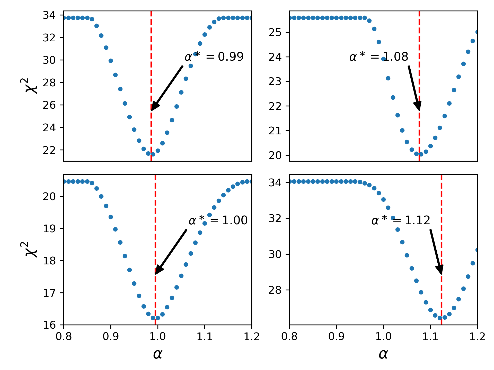
The left four panels of Fig. 13 show plots of variation of with for the four mock cuboids in L3.5 quarter-mock catalogue which correspond to distribution of halos without patchy reionization. In the right four panels of Fig 13, we show monopoles computed from Landy Szalay estimators and best fit monopoles () for the aforementioned mock cuboids. For the cuboids from L3.5 quarter-mock which correspond to the distribution of halos without patchy reionization, the values of minimum are 21.59, 20.03, 16.20, 26.42, and the values of are 0.99, 1.08, 1.00, 1.12 respectively. Hence, the mean values of minimum and are 21.06 and 1.05 respectively. The error on the BAO distance measurement is 0.032.
The plots in the left four panels of Fig. 14 illustrate the variations of with for the four mock cuboids in L3.5 quarter-mock catalogue which correspond to distribution of halos after applying patchy reionization. In the bottom two rows of Fig. 14, we show monopoles computed from Landy Szalay estimators and best fit monopoles () for these four mock cuboids. These cuboids have minimum values of of 38.80, 22.52, 43.14, 32.26 and best fit values of as 0.95, 0.99, 1.02, 0.98. As such, the mean values of minimum and are 34.18 and 0.98 respectively. The error on the BAO distance measurement is 0.014.


4.3 L1 mocks
The left four panels of Fig. 15 show plots of variations of with for the four mock cuboids in L1 quarter-mock catalogue which correspond to distribution of galaxies visible without patchy reionization. In the right four panels of Fig. 15, we show monopoles computed from Landy Szalay estimators and best fit monopoles () for the aforementioned mock cuboids. These cuboids have the following minimum values of : 19.49, 18.58, 11.79, 13.34. They have the following values of : 1.01, 1.03, 0.99, 0.95. Consequently the mean values of minimum and for these mock cuboids are 15.80 and 1.00 respectively. The fractional distance error is 0.015.
The left four panels of Fig. 16 illustrate the variations of with for the four mock cuboids in L1 quarter-mock catalogue which correspond to distribution of galaxies visible with patchy reionization. In the right four panels of Fig 16, we show monopoles computed from Landy Szalay estimators and best fit monopoles () for these four mock cuboids. The cuboids L1 quarter-mock catalogue which correspond to distribution of galaxies after patchy reionization have the following values of minimum : 12.33, 14.26, 15.67, 14.26. The values of for these cuboids are as follows: 0.96, 1.06, 1.01, 0.96. Hence, the mean values of minimum and for these mock cuboids are 14.13 and 1.00. The fractional distance error is 0.024.
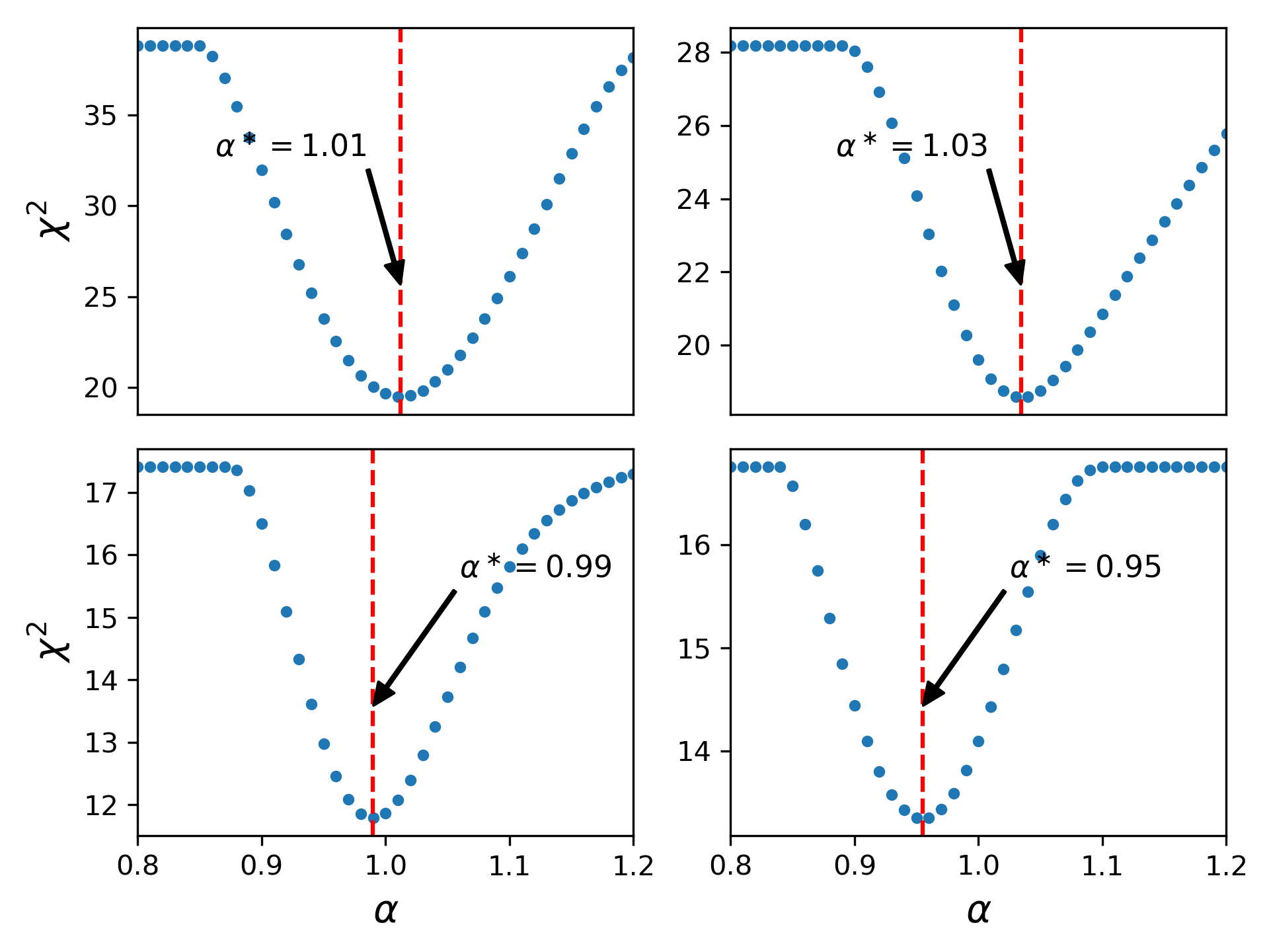


Table 3, gives summaries of our best fit results for all mocks in all three quarter-mock catalogues.
| Line detection | ||||
|---|---|---|---|---|
| sensitivity | (Mock 1) | (Mock 2) | (Mock 3) | (Mock 4) |
| Before patchy reionization | ||||
| erg/s/cm2 | 1.08 | 1.16 | 0.86 | 1.08 |
| erg/s/cm2 | 0.99 | 1.08 | 1.00 | 1.12 |
| erg/s/cm2 | 1.01 | 1.03 | 0.99 | 0.95 |
| With patchy reionization | ||||
| erg/s/cm2 | 1.04 | 0.81 | 1.05 | 1.19 |
| erg/s/cm2 | 0.95 | 0.99 | 1.02 | 0.98 |
| erg/s/cm2 | 0.96 | 1.06 | 1.01 | 0.96 |
| Line detection | ||||
| sensitivity | (Mock 1) | (Mock 2) | (Mock 3) | (Mock 4) |
| Before patchy reionization | ||||
| erg/s/cm2 | 27.41 | 31.32 | 28.17 | 45.86 |
| erg/s/cm2 | 21.59 | 20.03 | 16.20 | 26.42 |
| erg/s/cm2 | 19.49 | 18.58 | 11.79 | 13.34 |
| With patchy reionization | ||||
| erg/s/cm2 | 24.41 | 26.68 | 34.96 | 26.59 |
| erg/s/cm2 | 38.80 | 22.52 | 43.14 | 32.26 |
| erg/s/cm2 | 12.33 | 14.26 | 15.67 | 14.26 |
| Line detection | Mock 1 | Mock 2 | Mock 3 | Mock 4 |
|---|---|---|---|---|
| sensitivity | ||||
| erg/s/cm2 | 1.71 | 1.10 | 1.30 | 1.17 |
| erg/s/cm2 | 1.13 | 1.38 | 1.41 | 1.05 |
| erg/s/cm2 | 3.76 | 1.52 | 2.65 | 1.70 |
4.4 Analysis of errors on the BAO distance measurements
We now carry out an analysis of the BAO distance errors and their scatter, in order to check that they are statistically consistent. For the L7 quarter mock catalogues, we found the following values of best fit () from the four cuboids that represent the distribution of halos without patchy reionization: 1.08, 1.16, 0.86, 1.08. These values of lead to an overall fractional error of 0.064. At the same time, we observed the following values of in the four cuboids in the L7 quarter mock catalogues with patchy reionization : 1.04, 0.81, 1.05, 1.19. These values of yield an error of 0.079 on BAO distance measurement. To reconcile the scatter in the values of that we see for cuboids with and without patchy reionization, we carry out Fisher’s exact test (Fisher, 1922; Agresti, 1992). For each category of cuboids (with reionization or without), we are working with only four cuboids. This is a classic case of data with small sample sizes. Fisher’s exact test enables us to conduct accurate statistical significance tests on small samples. In this test, our null hypothesis is that there is no significant deviation in the distributions of the values of for cases with and without patchy reionization. A two-tailed Fisher exact hypothesis test for comparison of the distributions of the aforesaid values, gives us a p-value which is approximately 0.99. This p value is very high and it strongly suggests that we cannot ignore the null hypothesis.
Similarly, for L3.5 mocks, we have the following values of for halos without patchy reionization: 0.99, 1.08, 1.00, 1.12. For the four cuboids with patchy reionization, we have: 0.95, 0.99, 1.02, 0.98. We again conduct Fisher’s exact test. Our null hypothesis in this test is that there is no significant deviation in distributions of values of . From a two-tailed Fisher’s exact test, this time we get a p-value of approximately 1. This strongly suggests that there is significant evidence in support of our null hypothesis.
Finally, for L1 mocks, we get the following values of for halos without patchy reionization: 1.01, 1.03, 0.99, 0.95. When cuboids have patchy reionization, we get the following values of : 0.96, 1.06, 1.01, 0.96. A two-tailed Fisher’s exact test gives us a p-value of approximately 1, again strong evidence of the fact that there is no significant deviation in distributions of values of for cases with and without patchy reionization.
The results that we get from Fisher’s exact tests carried out on the mocks also suggest that we cannot make significant inferences from comparisons of scatter in values of in cuboids with patchy reionization and without patchy reionization.
4.5 Linear bias between in cases with and without reionization
The results that we see in Figures 12, 11, 14, 13, 16 and 15 suggest that the clustering amplitude changes somewhat significantly with and without reionization and also depends on the line strength. Equation 19 below defines the linear bias due to reionization compared to no reionization for a given cuboid. It is defined using a ratio of two galaxy correlation functions and is of course different from the usual linear bias of galaxies with respect to mass.
| (19) |
We tabulate the values of for cuboids in the L7, L3.5 and L1 mocks in Table 4. For the L7 mock catalogue, we obtain a mean of 1.32. We estimate the fractional errors on by computing the sample standard deviation of the results for the four quarter-mocks, and then dividing by to give the error on the mean. The fractional error computed this way is 0.136. In the case of the L3.5 mock catalogue, we get a mean of 1.24 and a fractional error of 0.089. Finally, for the four quarter-mocks in L1 mock catalogue, we obtain a mean of 2.41 and fractional error of 0.514. It is as we might expect: in all cases the effects of patchy reionization lead to higher amplitude clustering for the observable galaxies. The fainter galaxies (the L1 mocks) are also relatively much more strongly affected than the brighter galaxies.
5 Summary and Discussion
5.1 Summary
Using mock catalogues, we have investigated the prospect of utilizing the BAO feature at redshifts as a standard ruler. We have utilized four mock catalogues, each representing approximately one quarter of the volume that will be surveyed by RST with grism spectroscopy.
We see evidence for BAO peaks in three of the four mocks when we use the planned RST HLS Lyman- line detection sensitivity of . Hence, the BAO feature is likely detectable for this line detection sensitivity (measured in three out of four survey quadrants analysed independently). When we make mocks with better line detection sensitivities, we see evidence of BAO features in all mocks. For the standard line detection sensitivity, , we find a root mean square fractional distance error of 0.068 after comparison between mocks and fitted correlation function monopoles. For a factor of two fainter line detection sensitivity, , we find a distance error of 0.013. We find a distance error of 0.021 for mocks with line detection sensitivity .
5.2 Discussion
Our analysis of the use of BAO at high redshifts has included some of the relevant features and difficulties, such as non-linear clustering, redshift distortions, intrinsic galaxy line luminosities, and the effect of reionization bubbles. The results are promising, as we have summarised in Section 5.1 above. We have however left much for future work, including the visibility of the Lyman- line at these redshifts (including the effects of dust and the Lyman- damping wing), and the effects of interlopers and low redshift foregrounds. These factors could easily derail the possibility of measuring large-scale galaxy clustering at redshift , and should be investigated in detail. On the other hand, there are examples of galaxies being detected in Lyman- emission at these redshifts, for example the object by Tilvi et al. (2016), and from Larson et al. (2018). Even if the Lyman- emission line itself cannot be seen, the Lyman- break can also be used to spectroscopically identify galaxies, as was done using the HST grism at by Oesch et al. (2016). This could also be investigated to see whether it could enable clustering measurements at the BAO scale.
We have seen that the detectability of the BAO peak is just at the level of being possible with the fiducial flux limit of the RST HLS. To do this, we have already reduced the nominal 7 detection limit to 5 (). The exact survey design choices made when the RST mission is finalized will therefore be extremely relevant to whether the BAO measurement will be feasible. We have found that with a sensitivity a factor of two better the BAO can be seen clearly in four survey quadrants. This means that it could be advantageous to make use of smaller and deeper areas.
The analysis presented in this work was based on only 4 quarter-mocks for each of the tested line detection sensitivities. In the future, large number of mock catalogues should be generated to allow for the build up of a full covariance matrix for the correlation function. Because of the small number of mocks here, we were only able to use the diagonal elements of the covariance matrix in model fitting. As a result, the distance error estimates, which were derived from the scatter between mocks, were necessarily conservative. In a future work with large numbers of mocks, the extra information available from the off diagonal covariance matrix elements will mean that the fits to the BAO peaks will be improved and the distance errors will be somewhat reduced. The uncertainty in the distance error will also be better estimated. In the present case, the error on the error on the mean from only four quarter mocks will be large, and this is why the distance scale error on the L1 mocks increases to 2.4% from 1.4% for the L3.5 mocks, in spite of a factor of 3 increase in sensitivity.
In our treatment of reionization, we have assumed that galaxies which lie within ionized bubbles will be visible in Lyman- (consistent with the interpretation of Bagley et al. (2017)). We have compared the effects of including this patchy reionization, or not including it (all galaxies visible), and have found that the effect on BAO peak detection is quite small. For example, for the fiducial L7 sensitivity case, the effect of patchy reionization only increases the distance error from 6.4% to 7.9 %. This is likely to be because in the patchy model for reionization employed, overdense regions reionize first, and this is where most of the galaxy clustering signal lies. The reionization bubbles are also on smaller scales, than the BAO signal, and have a range of sizes, and therefore there is no masking of the BAO peak by bubbles. We note however that we have carried out no Lyman- radiative transfer on the scales of individual galaxies, and that the visibility or not of the line in different environments is likely to be much more complex than our simple bubble model.
One significant difference between the BAO measurements at redshifts and those for is the lack of non-linearities in gravitational clustering. For example we can see that in the right panels of Fig. 15 there is no obvious smoothing of the BAO peak compared to the linear CDM fit. This is an advantage of working at higher redshifts, as no reconstruction techniques (Sherwin & White, 2019) are needed to recover the maximum benefit. The high redshift galaxies do have a high bias (Bhowmick et al., 2019) and so their clustering is detectable where clustering of the density field would not be.
Measuring BAO in a new regime would at the very least be useful as a consistency check on measurements that have been made at low redshifts and in the CMB. It is important to fill in the large gap between the Lyman- forest measurements at (Aubourg et al., 2015) and the features seen at by Planck and WMAP (Planck Collaboration et al., 2018b; Bennett et al., 2013). Such measurements might shed some light on the tension between BAO and other Hubble parameter measurements (Cuceu et al., 2019), and whether early dark energy may be acting before the recombination epoch (Verde et al., 2019; Poulin et al., 2019).
One of the targets of cosmological analysis with the RST satellite is large scale structure measurements from galaxies at redshifts . This will extend the successful redshift space distortion, BAO, and other techniques to significantly earlier epochs than current large scale structure measurements from ground based surveys. Although much attention has rightly been focussed on this redshift range, we have seen in this paper that it may be possible to make an even greater leap, and use the large scale structure traced out by the very first massive galaxies as a cosmological probe. Although many potential pitfalls remain to be investigated, it is worth bearing this in mind when considering the RST survey strategies and parameters.
Acknowledgements
The BlueTides simulation was run on the BlueWaters facility at the National Center for Supercomputing Applications. TDM acknowledges funding from NSF ACI-1614853, NSF AST-1517593, NSF AST-1616168 and NASA ATP 19-ATP19-0084. TDM and RACC also acknowledge funding from NASA ATP 80NSSC18K101, and NASA ATP NNX17AK56G. RACC was supported by a Lyle Fellowship from the University of Melbourne, and TDM by a Shimmins Fellowship and a Lyle Fellowship from the University of Melbourne. G.R. acknowledges support from the National Research Foundation of Korea (NRF) through Grant No. 2017077508 funded by the Korean Ministry of Education, Science and Technology (MoEST), and from the faculty research fund of Sejong University in 2018. The work by KH was supported under the U.S. Department of Energy contract DE-AC02-06CH11357. This research used resources of the Argonne Leadership Computing Facility at the Argonne National Laboratory, which is supported by the Office of Science of the U.S. Department of Energy under Contract No. DE-AC02-06CH11357.
Data availability
The data underlying this article will be shared on reasonable request to the corresponding author.
References
- Agresti (1992) Agresti A., 1992, Statist. Sci., 7, 131
- Anderson et al. (2012) Anderson L., et al., 2012, Monthly Notices of the Royal Astronomical Society, 427, 3435
- Ansarinejad & Shanks (2018) Ansarinejad B., Shanks T., 2018, Monthly Notices of the Royal Astronomical Society, 479, 4091
- Ata et al. (2018) Ata M., et al., 2018, MNRAS, 473, 4773
- Aubourg et al. (2015) Aubourg É., et al., 2015, Phys. Rev. D, 92, 123516
- Bagley et al. (2017) Bagley M. B., et al., 2017, ApJ, 837, 11
- Battaglia et al. (2013) Battaglia N., Trac H., Cen R., Loeb A., 2013, The Astrophysical Journal, 776, 81
- Bautista et al. (2018) Bautista J. E., et al., 2018, ApJ, 863, 110
- Bennett et al. (2013) Bennett C. L., et al., 2013, ApJS, 208, 20
- Bertin & Arnouts (1996) Bertin E., Arnouts S., 1996, Astronomy and Astrophysics Supplement Series, 117, 393
- Bhowmick et al. (2019) Bhowmick A. K., Somerville R. S., DiMatteo T., Wilkins S., Feng Y., Tenneti A., 2019, arXiv e-prints, p. arXiv:1908.02787
- Bouwens et al. (2011) Bouwens R. J., et al., 2011, Nature, 469, 504
- Busca et al. (2013) Busca N. G., et al., 2013, A&A, 552, A96
- Casertano et al. (2015) Casertano S., Brammer G. B., Dixon V., Mackenty J. W., Pirzkal N., Ravindranath S., Ryan R. E., 2015, Technical report, Slitless Grism Spectroscopy with WFIRST: Observing Modes and Strategies, http://www.stsci.edu/files/live/sites/www/files/home/scientific-community/wfirst/{_}documents/WFIRST-STScI-TR1506A.pdf. http://www.stsci.edu/files/live/sites/www/files/home/scientific-community/wfirst/{_}documents/WFIRST-STScI-TR1506A.pdf
- Cassata, P. et al. (2011) Cassata, P. et al., 2011, A&A, 525, A143
- Chaikin et al. (2018) Chaikin E. A., Tyulneva N. V., Kaurov A. A., 2018, ApJ, 853, 81
- Colbert et al. (2018) Colbert J., et al., 2018, in American Astronomical Society Meeting Abstracts #231. p. 355.12
- Cole et al. (2005) Cole S., et al., 2005, MNRAS, 362, 505
- Comparat et al. (2016) Comparat J., et al., 2016, A&A, 592, A121
- Crocce & Scoccimarro (2008) Crocce M., Scoccimarro R., 2008, Phys. Rev. D, 77, 023533
- Cuceu et al. (2019) Cuceu A., Farr J., Lemos P., Font-Ribera A., 2019, J. Cosmology Astropart. Phys., 2019, 044
- Davis & Peebles (1983) Davis M., Peebles P. J. E., 1983, ApJ, 267, 465
- Davis et al. (1985) Davis M., Efstathiou G., Frenk C. S., White S. D. M., 1985, ApJ, 292, 371
- Eftekharzadeh et al. (2015) Eftekharzadeh S., et al., 2015, Monthly Notices of the Royal Astronomical Society, 453, 2779
- Eisenstein & Hu (1998) Eisenstein D. J., Hu W., 1998, ApJ, 496, 605
- Eisenstein et al. (2005) Eisenstein D. J., et al., 2005, ApJ, 633, 560
- Ellis et al. (2013) Ellis R. S., et al., 2013, ApJ, 763, L7
- Eyles et al. (2005) Eyles L. P., Bunker A. J., Stanway E. R., Lacy M., Ellis R. S., Doherty M., 2005, MNRAS, 364, 443
- Feng et al. (2015) Feng Y., Matteo T. D., Croft R., Tenneti A., Bird S., Battaglia N., Wilkins S., 2015, The Astrophysical Journal, 808, L17
- Feng et al. (2016) Feng Y., Di-Matteo T., Croft R. A., Bird S., Battaglia N., Wilkins S., 2016, Monthly Notices of the Royal Astronomical Society, 455, 2778
- Finkelstein et al. (2013) Finkelstein S. L., et al., 2013, Nature, 502, 524
- Fisher (1922) Fisher R. A., 1922, Journal of the Royal Statistical Society, 85, 87
- Fossati et al. (2017) Fossati M., et al., 2017, The Astrophysical Journal, 835, 153
- Francis et al. (2012) Francis P. J., Dopita M. A., Colbert J. W., Palunas P., Scarlata C., Teplitz H., Williger G. M., Woodgate B. E., 2012, Monthly Notices of the Royal Astronomical Society, 428, 28
- Gehrels et al. (2015) Gehrels N., Spergel D., WFIRST SDT Project 2015, in Journal of Physics Conference Series. p. 012007 (arXiv:1411.0313), doi:10.1088/1742-6596/610/1/012007
- Gronwall et al. (2007) Gronwall C., et al., 2007, The Astrophysical Journal, 667, 79
- Habib et al. (2013) Habib S., Morozov V., Frontiere N., Finkel H., Pope A., Heitmann K., 2013, in SC ’13: Proceedings of the International Conference on High Performance Computing, Networking, Storage and Analysis. pp 1–10, doi:10.1145/2503210.2504566
- Habib et al. (2016) Habib S., et al., 2016, New Astronomy, 42, 49
- Hamilton (1993) Hamilton A. J. S., 1993, ApJ, 417, 19
- Heitmann et al. (2019) Heitmann K., et al., 2019, arXiv e-prints, p. arXiv:1904.11970
- Hill & Baxter (2018) Hill J. C., Baxter E. J., 2018, J. Cosmology Astropart. Phys., 8, 037
- Hu et al. (2017) Hu W., et al., 2017, ApJ, 845, L16
- Kakiichi et al. (2016) Kakiichi K., Dijkstra M., Ciardi B., Graziani L., 2016, Monthly Notices of the Royal Astronomical Society, 463, 4019
- Kerscher et al. (2000) Kerscher M., Szapudi I., Szalay A. S., 2000, The Astrophysical Journal Letters, 535, L13
- Komatsu et al. (2011) Komatsu E., et al., 2011, Astrophysical Journal, Supplement Series, 192, 18
- Landy & Szalay (1993) Landy S. D., Szalay A. S., 1993, ApJ, 412, 64
- Laporte et al. (2017) Laporte N., et al., 2017, ApJ, 837, L21
- Larson et al. (2018) Larson R. L., et al., 2018, ApJ, 858, 94
- Lehnert et al. (2010) Lehnert M. D., et al., 2010, Nature, 467, 940
- Leitherer et al. (1999) Leitherer C., et al., 1999, ApJS, 123, 3
- Lewis & Bridle (2002) Lewis A., Bridle S., 2002, Phys. Rev. D, 66, 103511
- Li et al. (2019) Li N., et al., 2019, ApJ, 878, 122
- Malhotra (2019) Malhotra S., 2019, in American Astronomical Society Meeting Abstracts. p. 315.01
- McCarthy et al. (1999) McCarthy P. J., et al., 1999, The Astrophysical Journal, 520, 548
- Mobasher et al. (2005) Mobasher B., et al., 2005, ApJ, 635, 832
- Oesch et al. (2016) Oesch P. A., et al., 2016, ApJ, 819, 129
- Pentericci et al. (2018) Pentericci L., et al., 2018, A&A, 619, A147
- Planck Collaboration et al. (2018a) Planck Collaboration et al., 2018a, arXiv e-prints,
- Planck Collaboration et al. (2018b) Planck Collaboration et al., 2018b, arXiv e-prints, p. arXiv:1807.06209
- Pons-Bordería et al. (1999) Pons-Bordería M.-J., Martínez V. J., Stoyan D., Stoyan H., Saar E., 1999, ApJ, 523, 480
- Poulin et al. (2019) Poulin V., Smith T. L., Karwal T., Kamionkowski M., 2019, Phys. Rev. Lett., 122, 221301
- Raichoor et al. (2017) Raichoor A., et al., 2017, MNRAS, 471, 3955
- Riess et al. (2018) Riess A. G., et al., 2018, ApJ, 855, 136
- Sarpa et al. (2019) Sarpa E., Schimd C., Branchini E., Matarrese S., 2019, MNRAS, 484, 3818
- Sherwin & White (2019) Sherwin B. D., White M., 2019, J. Cosmology Astropart. Phys., 2019, 027
- Slosar et al. (2013) Slosar A., et al., 2013, J. Cosmology Astropart. Phys., 4, 026
- Sobacchi & Mesinger (2015) Sobacchi E., Mesinger A., 2015, Monthly Notices of the Royal Astronomical Society, 453, 1843
- Song et al. (2016) Song M., Finkelstein S. L., Livermore R. C., Capak P. L., Dickinson M., Fontana A., 2016, The Astrophysical Journal, 826, 113
- Spergel et al. (2015) Spergel D., et al., 2015, arXiv e-prints, p. arXiv:1503.03757
- Tilvi et al. (2010) Tilvi V., et al., 2010, The Astrophysical Journal, 721, 1853
- Tilvi et al. (2016) Tilvi V., et al., 2016, ApJ, 827, L14
- Vanderlinde & Chime Collaboration (2014) Vanderlinde K., Chime Collaboration 2014, in Exascale Radio Astronomy.
- Vargas-Magaña et al. (2014) Vargas-Magaña M., et al., 2014, Monthly Notices of the Royal Astronomical Society, 445, 2
- Verde et al. (2019) Verde L., Treu T., Riess A. G., 2019, Nature Astronomy, 3, 891
- Wang et al. (2014) Wang M.-Y., Peter A. H. G., Strigari L. E., Zentner A. R., Arant B., Garrison-Kimmel S., Rocha M., 2014, MNRAS, 445, 614
- Waters et al. (2016) Waters D., Di Matteo T., Feng Y., Wilkins S. M., Croft R. A. C., 2016, MNRAS, 463, 3520
- Weinberg et al. (2013) Weinberg D. H., Mortonson M. J., Eisenstein D. J., Hirata C., Riess A. G., Rozo E., 2013, Phys. Rep., 530, 87
- Wilkins et al. (2013) Wilkins S. M., et al., 2013, Monthly Notices of the Royal Astronomical Society, 435, 2885
- Wilkins et al. (2016a) Wilkins S. M., Feng Y., Di-Matteo T., Croft R., Stanway E. R., Bouwens R. J., Thomas P., 2016a, MNRAS, 458, L6
- Wilkins et al. (2016b) Wilkins S. M., Feng Y., Di-Matteo T., Croft R., Stanway E. R., Bunker A., Waters D., Lovell C., 2016b, MNRAS, 460, 3170
- Wilkins et al. (2017) Wilkins S. M., Feng Y., Di Matteo T., Croft R., Lovell C. C., Waters D., 2017, MNRAS, 469, 2517
- Wilkins et al. (2019) Wilkins S. M., et al., 2019, arXiv e-prints, p. arXiv:1904.07504
- Xu et al. (2012) Xu X., Padmanabhan N., Eisenstein D. J., Mehta K. T., Cuesta A. J., 2012, MNRAS, 427, 2146
- Xu et al. (2013) Xu X., Cuesta A. J., Padmanabhan N., Eisenstein D. J., McBride C. K., 2013, MNRAS, 431, 2834
- Yajima et al. (2018) Yajima H., Sugimura K., Hasegawa K., 2018, Monthly Notices of the Royal Astronomical Society, 477, 5406
- Yan et al. (2011) Yan H., et al., 2011, ApJ, 728, L22
- Zarrouk et al. (2018) Zarrouk P., et al., 2018, Monthly Notices of the Royal Astronomical Society, 477, 1639
- Zhai et al. (2017) Zhai Z., et al., 2017, ApJ, 848, 76
- de Sainte Agathe et al. (2019) de Sainte Agathe V., et al., 2019, A&A, 629, A85
- du Mas des Bourboux et al. (2017) du Mas des Bourboux H., et al., 2017, A&A, 608, A130