On the Parallelizability of Approval-Based Committee Rules

Zack Fitzsimmons
Dept. of Math. and Computer Science
College of the Holy Cross
Worcester, MA 01610 Zohair Raza Hassan
Department of Computer Science
Rochester Institute of Technology
Rochester, NY 14623 Edith Hemaspaandra
Department of Computer Science
Rochester Institute of Technology
Rochester, NY 14623

(January 24, 2025)

Abstract

Approval-Based Committee (ABC) rules are an important tool for choosing a fair set of candidates when given the preferences of a collection of voters. Though finding a winning committee for many ABC rules is NP-hard, natural variations for these rules with polynomial-time algorithms exist. The Method of Equal Shares, an important ABC rule with desirable properties, is also computable in polynomial time. However, when working with very large elections, polynomial time is not enough and parallelization may be necessary. We show that computing a winning committee using these ABC rules (including the Method of Equal Shares) is P-hard, thus showing they cannot be parallelized. In contrast, we show that finding a winning committee can be parallelized when the votes are single-peaked or single-crossing for the important ABC rule Chamberlin-Courant.

1 Introduction and Related Work

Elections are a widely-used tool for a group of agents to reach a collective decision. Multiwinner voting rules are used for elections where instead of a single winner, the desired outcome is a set of winners of a given size (see Faliszewski et al. (2017)). Approval-based committee (ABC) rules are an important and widely-studied type of multiwinner rule (see Lackner and Skowron (2023)), where voters express dichotomous preferences (approval/disapproval) over the set of candidates.

Finding a winning committee for many ABC rules is NP-hard (LeGrand et al., 2007; Procaccia et al., 2008; Aziz et al., 2015; Skowron et al., 2016; Godziszewski et al., 2021; Brill et al., 2024). However, natural variations of these NP-hard rules exist where a winning set of candidates can be found in polynomial time. In addition, the Method of Equal Shares, which has the desirable property of electing a committee that satisfies Extended Justified Representation, can be computed in polynomial time (Peters and Skowron, 2020).

It is important that we can always easily compute the outcome of an election. Previous work on studying the complexity of winner determination has largely focused on whether the winner problem is in P or NP-hard, equating being in P with being easy to compute. However, when elections are very large it is not enough to just have a polynomial-time algorithm. In this case parallelization may be necessary.

The parallelizability of voting rules was previously considered for single-winner voting rules (Csar et al., 2018, 2017), but not for the case of multiwinner rules. In fact, the recent textbook on ABC rules by Lackner and Skowron (2023) explicitly includes as open question “Q20” to determine which polynomial-time ABC rules are inherently sequential. As pointed out by Lackner and Skowron (2023), Approval Voting (AV) is clearly parallelizable (and the analogous result for Satisfaction Approval Voting (SAV) follows from the same argument). We show that computing the winning committee for all other studied polynomial-time ABC rules is inherently sequential.

To show that a problem is inherently sequential we use the notion of P-hardness, since it is generally assumed that P-hard problems are not parallelizable (Greenlaw et al., 1995). We mention that this approach was used previously in computational social choice to show results about single-winner elections (specifically that winner determination for resolute versions of STV and Ranked Pairs is P-complete) (Csar et al., 2017, 2018), problems related to the aggregation of CP-nets (Lukasiewicz and Malizia, 2022), and for finding the essential set (Brandt and Fischer, 2008).

When studying the complexity of a voting problem it is natural to consider settings where the votes of the electorate have structure. Two important domain restrictions are single-peaked and single-crossing preferences (Black, 1948; Mirrlees, 1971), which each model settings where the votes of the electorate are based on a single dimension (e.g., liberal vs. conservative). Both of these models have natural counterparts for approval voting (Faliszewski et al., 2011; Elkind and Lackner, 2015). We show that for single-peaked and for single-crossing approval votes finding a winning committee using the important Chamberlin-Courant ABC rule can be parallelized. We note here that the only previously-known parallelizability results for voting rules that we are aware of (in addition to AV and SAV mentioned previously (Lackner and Skowron, 2023)) are the one for Schultze Voting (Csar et al., 2018) as well as computing the Copeland, Smith, and Schwartz choice sets (Brandt et al., 2009).

Our main contributions are summarized below.

Inherently sequential ABC rules. We provide P-hardness reductions to prove the following theorem which encompasses all studied polynomial-time ABC rules from (Lackner and Skowron, 2023) except AV and SAV which are easily seen to be parallelizable (Lackner and Skowron, 2023); in fact they are computable in logarithmic space (see Section A of the appendix for completeness).

Theorem 1.

Computing a winning committee is inherently sequential for seq-CC, seq-PAV, rev-seq-CC, rev-seq-PAV, seq-Phragmén, Greedy Monroe, and the Method of Equal Shares.

We show that seq-CC and the Method of Equal Shares are inherently sequential in Section 3. The remaining rules are discussed in Section C of the appendix. In fact, we show that some of these rules are special cases of an infinite class of rules that we prove the P-hardness of.

Parallelizability under domain restrictions. For the well-studied domain restrictions of single-peaked and single-crossing approval votes, we show that finding a winning committee for the important multiwinner rule Chamberlin-Courant can be parallelized (see Section 4).

Instead of providing parallel algorithms, we show membership in the relatively unknown complexity class OptL from Álvarez and Jenner (1993) (Definition 14). This allows for stronger results (since OptL is thought to be a strict subset of the class of parallelizable problems) and simpler proofs (since describing parallel algorithms can be an arduous task, e.g., one has to decide on a model and describe how each machine aggregates information, etc.).

To the best of our knowledge, we are the first to use this class to show parallelizability, and we expect that this approach will be useful to further explore the parallelizability of other polynomial-time problems.

2 Preliminaries

2.1 Approval-Based Committee (ABC) Rules

An approval-based committee election consists of a set of candidates $C$ , a collection of votes $V$ where each $v\in V$ is a set of approved candidates, and a desired committee size $k\in\mathbb{N}$ . The output of an approval-based committee rule is a set of $k$ candidates referred to as the winning committee.

We study a large number of ABC rules, which we generally define either where they are first used or in the appendix. We present the formal definition of Chamberlin-Courant (Chamberlin and Courant, 1983) below since it will be relevant for results in Section 3.1 and Section 4, and it allows us to provide an illustrative example below.

Definition 2 (Chamberlin-Courant (CC)).

Given candidates $C$ , collection of votes $V$ , and committee size $k$ , output a committee $W$ of size $k$ such that the most votes have at least one approved candidate in the committee.

Example 3.

Suppose we have candidates $C=\{a,b,c\}$ , committee size $k=2$ , and the following collection of votes:

V=\left[\begin{array}[]{cccccc}\{a\},&\{a,c\},&\{a,c\},&\{b,c\},&\{b,c\},&\{b\}\end{array}\right]

The winning committee computed by CC is $\{a,b\}$ , since the maximum number of voters (in this case, all voters) approve of a candidate in $\{a,b\}$ .

2.2 Computational Complexity

Most of our results concern showing problems to be inherently sequential. It is widely believed that problems that are P-hard are inherently sequential (Greenlaw et al., 1995). Note that when showing a problem is hard for a given complexity class we must be careful to use a reduction with less computational power than the class we are showing hardness for. As is standard we use logspace reductions for our P-hardness results, meaning that the reduction is computable in logarithmic space.¹¹1Though logarithmic space may seem quite restrictive, standard NP-hardness reductions are computable in logarithmic space.

Most standard complexity classes such as P and NP are concerned with decision problems, whose algorithms accept or reject inputs. However, we want to output the winning committee for ABC rules, i.e., we are looking at function problems, and so we need to also look at function complexity classes.

The complexity class NC (and its function counterpart FNC) corresponds to the class of problems that have (efficient) parallel algorithms, namely, algorithms that run in polylogarithmic time using a polynomial number of processors (see Papadimitriou (1994)).

It is easy to see that FNC is a subset of FP, the function counterpart of P. Our results that show problems inherently sequential are based on the generally accepted assumption that ${\rm FNC}\neq{\rm FP}$ , and we show inclusion in FNC for parallelizability.

3 Inherently Sequential ABC Rules

This section establishes the P-hardness of ABC rules. We highlight Chamberlin-Courant (CC) and the Method of Equal Shares (MES), while the P-hardness results for other ABC rules are deferred to the appendix. Before we present our proofs, we discuss an important technical consideration.

Recall that finding the winning committee is a function problem. However, it gives more insight to prove the hardness of a related decision problem. Thus, we consider the decision problem that asks about the containment of a single candidate. First, we show that this formulation is correct by showing the equivalence of the decision and function problem with respect to parallelizability.

Observation 4.

Suppose we are given a set of candidates $C$ , collection of votes $V$ , committee size $k$ , and a candidate $c\in C$ . For any ABC rule, finding the winning committee $W$ is parallelizable if and only if deciding whether $c$ belongs to $W$ is parallelizable.

Proof.

Suppose there is a parallel algorithm $X$ that outputs the winning committee $W$ . Then, one can run $X$ to find $W$ and simply check whether $c\in W$ to accept/reject for the decision problem. Now, suppose there is a parallel algorithm $X$ that decides whether $c$ belongs to $W$ . In this case, one can run $X$ for each candidate in parallel and output the $k$ candidates for which $X$ accepts. ∎

3.1 Chamberlin-Courant

Recall that the Chamberlin-Courant rule picks $k$ candidates that hit the most number of votes; a vote is “hit” if at least one of the candidates it approves is selected in the winning committee.

While computing the winning committee for CC is NP-hard (Procaccia et al., 2008) in the general case, simple greedy approaches have been introduced to mimic CC in polynomial time. One such approach is the sequential Chamberlin-Courant rule, denoted seq-CC, where we start with an empty committee and iteratively add the candidate that increases the number of currently hit votes the most (see (Lackner and Skowron, 2023)).

Definition 5 (seq-CC).

Suppose we are given candidates $C$ , collection of votes $V$ , and committee size $k$ . seq-CC sequentially builds a committee of size $k$ by repeatedly picking the candidate that increases the number of hit votes the most. Ties are broken lexicographically.

We will show that computing the winning committee using seq-CC is P-hard. Specifically, we show that deciding whether a given candidate is picked for the seq-CC winning committee is P-hard. To do this, we give a logspace reduction from a closely related P-complete problem, OVR, defined below. We note that as with NP-hardness reductions, half the battle is finding the right problem to reduce from, and we were able to find a problem almost equivalent to seq-CC. We hope that the the straightforward nature of our reduction will ease the reader into P-hardness reductions.

Problem 6 (Ordered Vertices Remaining (OVR) (Greenlaw, 1989)).

We are given an undirected graph $G$ , a vertex $v\in V(G)$ , and an integer $k$ . Suppose we repeatedly delete the highest-degree vertex from $G$ until no vertices remain—ties are broken lexicographically. Decide whether there are at least $k$ vertices remaining after deleting $v$ .

Theorem 7.

Computing the winning committee for seq-CC is inherently sequential.

Proof.

Suppose we are given an instance, $(G,v,k)$ , of OVR. We will construct an election with candidates $C$ , collection of votes $V$ , and committee size $k^{\prime}$ , and specify a candidate $c$ such that the winning committee selected by seq-CC includes $c$ if and only if $k$ vertices remain after $v$ is deleted. We provide an example of our reduction in Figure 1.

Let $C$ have a candidate for each vertex of $G$ , and let $V$ have a vote for each edge such that edge $\{a,b\}\in E(G)$ corresponds to a vote for candidates $a$ and $b$ . Finally, we set $c=v$ and $k^{\prime}=\|V(G)\|-k$ .

Recall that during each round of seq-CC, we pick the candidate that hits the most new votes. Similarly in OVR, we delete the vertex with highest degree. In our reduction, the vertex of the highest degree corresponds exactly to the candidate that hits the most unhit votes. Thus, if $v$ is among the first $\|V(G)\|-k$ candidates selected with seq-CC, then there must be at least $k$ vertices remaining in $G$ after deleting $v$ in OVR.

The reduction is clearly in logspace since we are essentially just copying the input and computing $k^{\prime}$ . ∎

Refer to caption — Figure 1: Column (a) shows the graph input to OVR at the top and the corresponding seq-CC election at the bottom. Columns (b) and (c) show the state of OVR and seq-CC after one and two rounds, respectively. Candidates are underlined when they are put in the winning committee and votes are darkened when they are hit. Observe how the removal of the highest-degree vertex in OVR corresponds to its inclusion in the winning committee in seq-CC.

We will see in Section C.1 of the appendix that a reduction from a different problem provides a more general result; there we analyze the P-hardness of a class of rules, which includes seq-CC, known as sequential Thiele methods. However, we decided to include the reduction from OVR to provide a simple, illustrative P-hardness proof in the main text.

3.2 Method of Equal Shares

The Method of Equal Shares (MES) is a recently introduced rule (Peters and Skowron, 2020) that allots voters budgets and allows them to elect candidates using shares of their budget. This rule has many desirable properties. In particular, it satisfies Extended Justified Representation (a notion of group fairness) and is computable in polynomial time. A generalized version of this rule (Peters et al., 2021), has also been used in the real world for participatory budgeting (a setting that generalizes multiwinner elections to voting over issues to be funded) (see (Peters and Skowron, 2024)).

Since the definition of MES is quite involved, we first provide an informal description, followed by an example, and finally, the formal definition.

In an MES election, voters are given a budget that they can use to elect candidates they approve of, provided they can afford it. The election proceeds in rounds, wherein a candidate is added to the winning committee by the end of each round. Adding a candidate $c$ to the winning committee incurs a cost of 1, which is split among all voters who approve of $c$ . The candidate chosen is the one that minimizes the maximum cost incurred by each voter approving them. Once a candidate is elected, each voter’s budget is adjusted according to the cost they paid to elect said candidate. The process continues until $k$ candidates have been elected, or until voters no longer possess the budget to elect a new candidate.

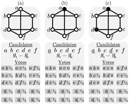
Example 8.

Suppose we have candidates $\{a,b,c,d\}$ and $n=4$ voters, labeled $1$ to $4$ , who want to elect a committee of size $k=3$ . Each voter starts with an initial budget of $k/n=3/4$ . The votes and budgets of each voter are:

\begin{array}[]{ccc|ccc}1:&\{a,c\}&\nicefrac{{3}}{{4}}&2:&\{a,c\}&\nicefrac{{3}}{{4}}\\ 3:&\{a,b\}&\nicefrac{{3}}{{4}}&4:&\{b,d\}&\nicefrac{{3}}{{4}}\end{array}

Candidates require a cost of 1 to be elected. Candidate $a$ can be elected if all of its voters pay $1/3$ . Candidate $b$ can be elected if all of its voters pay $1/2$ . Candidate $c$ can be elected if all of its voters pay $1/2$ . Candidate $d$ can be elected if voter 4 pays 1, but this is not possible since the voter does not have the budget. MES looks to minimize the maximum cost incurred by each voter; so in this case, it will pick candidate $a$ for the winning committee, since said cost is $1/3$ . The cost incurred by each voter is subtracted and we are left with the following budgets:

\begin{array}[]{ccc|ccc}1:&\{a,c\}&\nicefrac{{5}}{{12}}&2:&\{a,c\}&\nicefrac{{5}}{{12}}\\ 3:&\{a,b\}&\nicefrac{{5}}{{12}}&4:&\{b,d\}&\nicefrac{{3}}{{4}}\end{array}

Candidate $c$ can no longer be elected since its voters, 1 and 2, have a total budget of $10/12<1$ . Candidate $b$ ’s voters have a total budget of $7/6$ , so $b$ can be elected. The maximum budget paid by each of $b$ ’s voters is minimized if voter 4 pays $7/12$ and voter 3 pays $5/12$ . Thus, MES elects $b$ , and the updated budgets are:

\begin{array}[]{ccc|ccc}1:&\{a,c\}&\nicefrac{{5}}{{12}}&2:&\{a,c\}&\nicefrac{{5}}{{12}}\\ 3:&\{a,b\}&0&4:&\{b,d\}&\nicefrac{{1}}{{6}}\end{array}

MES terminates here and returns the committee $\{a,b\}$ as the cost to elect candidates $c$ or $d$ cannot be met by its voters. Note that MES returns fewer candidates than the desired committee size. This is discussed further below.

We now formally define the rule, heavily based on the definition from Lackner and Skowron (2023).

Definition 9 (Method of Equal Shares (MES)).

Suppose we are given candidates $C$ , collection of votes $V$ , and committee size $k$ . We will assume that there are $n$ votes and each voter is identified with an integer in $[1,n]$ .

Let $x_{r}(i)$ be the budget of voter $i$ at the end of round $r$ ; $x_{0}(i)=k/n$ . Suppose we are electing a candidate in round $r+1$ . Let $C_{r}$ be the candidates that can be elected; candidates that have not already been selected for the winning committee and whose voters can afford to elect them, i.e., $\sum_{i\in N(c)}x_{r}(i)\geq 1$ , where $N(c)$ is the set of voters that approve of $c$ . We select a new candidate like so. For each candidate $c\in C_{r}$ , we compute $\rho_{c}$ : the minimum value such that each voter approving $c$ pays at most $\rho_{c}$ and all voters pay a total of 1, i.e., we compute the minimum value $\rho_{c}$ satisfying:

\sum_{i\in N(c)}\min(x_{r}(i),\rho_{c})=1

The candidate with minimum $\rho_{c}$ is selected for the winning committee—ties are broken lexicographically. The budgets for each voter are updated as follows:

x_{r+1}(i)=\begin{cases}x_{r}(i)-\rho_{c}&\text{if $i$ approves $c$ and $x_{r}(i)\geq\rho_{c}$}\\ 0&\text{if $i$ approves $c$ and $x_{r}(i)<\rho_{c}$}\\ x_{r}(i)&\text{otherwise}\end{cases}

Note that voters may run out of the budget necessary to elect another candidate before $k$ rounds. In this case, the method terminates early and returns the winning committee constructed so far. However, technically this does not meet our definition of an ABC rule, since we must return a committee of size $k$ . To rectify this, another ABC rule is called to select the remaining candidates. Lackner and Skowron (2023) suggest using seq-Phragmén (see Sections C.2 and C.4 of the appendix) since it preserves some desirable properties.

We will show that computing the committee found by MES is P-hard. This shows that the hardness of MES is not caused by the hardness of the rule called afterward (such as seq-Phragmén). As in the previous section, we focus on the decision problem where we ask about the inclusion of a specified candidate. We reduce from a problem known as LFMIS:

Problem 10 (Lexicographically First Maximal Independent Set (LFMIS) (Cook, 1985)).

Suppose we are given an undirected graph $G$ and a vertex $v$ . The LFMIS of $G$ is a maximal independent set built by repeatedly picking the lexicographically first vertex not adjacent to an already picked vertex until no more vertices can be added. Decide if $v$ belongs to the LFMIS of $G$ .

For reasons that will be made clear in the upcoming proof, working with regular graphs (graphs where each vertex has the same degree) allows for a much easier hardness reduction. Miyano (1989) showed that LFMIS is P-complete even when the input graph is subcubic, i.e., each vertex has degree at most three. In Section B of the appendix, we show how this result can be easily extended to show that LFMIS is P-complete even when the input graph is 3-regular. Thus, for our proof below, we will assume that is the case.

Theorem 11.

Computing the winning committee for MES is inherently sequential.

Proof.

Suppose we are given an instance $(G,v)$ of LFMIS, where $G$ is a 3-regular graph with $m$ vertices labeled $1$ to $m$ . We will construct an election with candidate $C$ , collection of votes $V$ , and committee size $k$ , and specify a candidate $c\in C$ such that the winning committee selected by MES includes $c$ if and only if $v$ is included in the LFMIS of $G$ .

Similar to the proof of Theorem 7, let $C$ have a candidate for each vertex of $G$ , and $V$ have a vote for each edge such that edge $\{a,b\}\in E(G)$ corresponds to a vote for candidates $a$ and $b$ . We also add $m$ extra candidates to $C$ , labeled $m+1$ to $2m$ , with three singleton votes in $V$ for each. Observe that the lexicographic order of the input graph is preserved in our election. Note that we have a total of $n=3m/2+3m$ votes. Finally, we set $c=v$ and $k=m/2+m$ .

We now show that the candidates corresponding to $V(G)$ picked by MES correspond exactly to the vertices in the LFMIS of $G$ . This is illustrated with an example in Figure 2.

Observe that the initial budget is

x_{0}(i)=\frac{k}{n}=\frac{m/2+m}{3m/2+3m}=\frac{1}{3}

for each voter $i$ . Also, recall that each candidate has exactly three votes. At the start of round 1, any candidate $c\in C$ can be elected, since its three supporters can each pay $1/3$ to elect it. $1/3$ is also the minimum amount, $p_{c}$ , that can be paid by each voter to achieve this. Due to lexicographic tie-breaking, we will select the candidate labeled 1. When updating our budget for the next round, observe that any voter $i$ approving candidate 1 now has a remaining budget of 0; $x_{1}(i)=x_{0}(i)-\rho_{c}=1/3-1/3=0$ .

Due to this decreased budget, in the next round, any candidate that shared a vote with candidate 1 cannot be elected since its voters can no longer afford to pay for them. This corresponds exactly to LFMIS, wherein any vertex adjacent to an already selected vertex cannot be added to the independent set. Thus, in subsequent rounds, a candidate who does not share a vote with a previously elected candidate must be elected. It is now easy to see that the candidates corresponding to vertices in $G$ picked by MES correspond exactly to the vertices in the LFMIS of $G$ .

Note that since $k$ is large enough (more than the number of vertices of $G$ ), all of the vertices in the LFMIS will be picked. The extra candidates, $m+1$ to $2m$ , will be picked after LFMIS candidates due to lexicographic ordering. Note that since each extra candidate also has exactly three voters, the minimum budget to elect them, $\rho_{c}$ , is also $1/3$ . It should now be clear that these extra candidates were added so that our initial budget is $1/3$ .

It is clear that $v\in V(G)$ is elected by MES if and only if $v$ is part of $G$ ’s LFMIS, and that the reduction is clearly in logspace, thus completing our proof. ∎

We note that the reduction above may return a winning committee with fewer than $k$ candidates. Recall that in this case another ABC rule is called to elect the remaining candidates. For the sake of completeness, we show in Section C.4 of our appendix that MES is also P-hard when seq-Phragmén is used, as suggested by Lackner and Skowron (2023), to finish electing a total of $k$ candidates. Particularly, we reduce from LFMIS and show that the specified vertex $v$ is picked by MES if and only if $v$ belongs to the LFMIS.

4 Domain Restrictions

We now turn our attention to domain restrictions. Such restrictions often result in axiomatic and computational advantages (see, e.g., Elkind et al. (2017)). The most commonly studied domain restrictions are single-peaked preferences (Black, 1948) and single-crossing preferences (Mirrlees, 1971). Each of these restrictions capture natural settings where the electorates are focused on a single issue. In single-peakedness, this results in an ordering of the candidates from one extreme to the other, while in a single-crossing electorate the voters are ordered with respect to this issue and voters on either end represent the extremes. These restrictions were each first defined for preference order ballots, but have natural definitions for approval votes. Faliszewski et al. (2011) introduced the model of single-peakedness for approval ballots, and Elkind and Lackner (2015) introduced the model of single-crossingness for approval ballots.

A collection of (approval) votes is single-peaked if there exists a linear order of the candidates (a single-peaked axis) such that each vote forms a contiguous interval on the axis (Faliszewski et al., 2011) (this is also known as candidate interval (CI) (Elkind and Lackner, 2015)). A collection of (approval) votes is single-crossing if there exists a linear order of the voters (a single-crossing axis) such that for each candidate the set of voters that approve that candidate forms a contiguous interval on the axis (this is also known as voter interval (VI)) (Elkind and Lackner, 2015). See Figure 3 for an example of an election whose votes are both single-peaked and single-crossing.

As pointed out by Faliszewski et al. (2011) (for single-peaked) and Elkind and Lackner (2015) (for single-crossing), the problem of determining whether a collection of votes (in our setting of approval ballots) is single-peaked or single-crossing, and computing an axis witnessing this is in essence the problem of determining whether a 0-1 matrix has the consecutive ones property and computing a permutation that witnesses that. These problems have long been known to be computable in polynomial time (Fulkerson and Gross, 1965; Booth and Lueker, 1976).

Algorithms for these domain restrictions typically start with computing an axis. Since we are interested in complexity classes below P, we need to look at the complexity of computing an axis in more detail. Careful inspection of the literature shows that computing whether a 0-1 matrix has the consecutive ones property and computing a permutation that witnesses that is in fact computable in logarithmic space (Köbler et al., 2011). This immediately gives us the novel observation that computing whether a collection of votes (in our setting of approval ballots) is single-peaked or single-crossing and computing an axis witnessing this is computable in logarithmic space. We note that this claim also holds in the common setting where the votes are preference orders. This follows from observing that the reductions to the consecutive ones problem (Bartholdi and Trick, 1986; Bredereck et al., 2013) are easily seen to be computable in logarithmic space.

Observation 12.

Computing whether a collection of votes is single-peaked or single-crossing and computing an axis witnessing this is computable in logarithmic space. This holds in our setting of approval ballots as well as in the setting of preference order ballots.

As mentioned previously, domain restrictions can lower complexity. This is also the case in our context of approval ballots. For example, finding a winning committee for Chamberlain-Courant is NP-hard (Procaccia et al., 2008, Theorem 1), but for single-peaked votes and for single-crossing votes, this problem is computable in polynomial time (Betzler et al., 2013; Elkind and Lackner, 2015).

We use SP-CC (resp., SC-CC) to refer to the problems of computing a CC committee when the votes are single-peaked (resp., single-crossing). In contrast to the results of the previous section, we will show that these problems are even parallelizable.

Theorem 13.

SP-CC and SC-CC are parallelizable.

We will show that SP-CC and SC-CC are in some sense computable in nondeterministic logarithmic space, in a way that will imply that these problems are parallelizable. When looking at deterministic complexity classes, it is a little sloppy but not dangerous to talk about function problems (such as computing the winning coalition) as being in a complexity class like P (really a class of decision problems). However, we need to be very careful when talking about nondeterministic function classes, since such functions are inherently multi-valued, while we are interested in single-valued functions. There are multiple ways to get from multi-valued to single-valued functions. We will use the simplest way for our purposes: the function class OptL (Álvarez and Jenner, 1993).

Definition 14 (OptL).

OptL is the class of functions computable by taking the maximum of the output values over all accepting paths of an NL transducer, i.e., a nondeterministic Turing machine with a read-only input tape, a logspace work tape, and a write-only output tape.

We provide a visualization in Figure 4. It is known that every OptL function is parallelizable (Álvarez and Jenner, 1993, Theorem 4.2). We will show that SP-CC and SC-CC are in OptL (Theorems 15 and 16), which immediately implies Theorem 13.

Since we can compute an SC or SP axis in logarithmic space, we will see that our problems are in essence interval problems, with SP-CC corresponding to computing a set of $k$ points (candidates) that hit the most intervals (voters) and SC-CC corresponding to computing a set of $k$ intervals (with each interval being the set of voters that approve a particular candidate) whose union (the set of voters that approve at least one of those candidates) is as large as possible.

Theorem 15.

SP-CC is in OptL.

Proof.

Assume that there are $m$ candidates and $n$ voters. Recall that a collection of votes is single-peaked if there exists a linear order of the candidates (a single-peaked axis) such that each vote forms a contiguous interval on the axis. Let $L$ be the single-peaked axis given by the logarithmic space algorithm that computes an SP axis.

For $1\leq i\leq n$ , let $[s_{i},t_{i}]$ be the interval corresponding to the $i$ th voter, i.e., $s_{i}$ and $t_{i}$ are in $\{1,\ldots,m\}$ and the $i$ th voter approves the candidates from the $s_{i}$ th candidate to the $t_{i}$ th candidate on our SP axis $L$ . Note that we can’t store all these values, but we can recompute each value in logarithmic space whenever it is needed.

We now need to compute a set of $k$ candidates that hit (have nonempty intersection with) the most voters (intervals). We only keep track of the last candidate ( $lastc$ ) and the next candidate chosen ( $nextc$ ), the number of candidates selected so far ( $numc$ ), the number of voters hit so far ( $numv$ ), and a counter to iterate through the voters ( $i$ ). We also need to make sure that the maximum output value corresponds to a set of $k$ candidates that hits the most voters ( $optv$ ). Our algorithm is presented in Algorithm 1.

Algorithm 1 SP-CC

1: guess

optv\leq n

2: append

1^{optv\cdot m(m+1)}0

to output

lastc=0

;

numv=0

4: for

numc=1

k

5: guess

nextc

such that

lastc<nextc\leq m

6: reject if

lastc\geq m

numv

\|\{[s_{i},t_{i}]\ |\ s_{i}>lastc\text{ and }nextc\in[s_{i},t_{i}]\}\|

lastc=nextc

9: append

1^{lastc}0

to output

10: end for

11: accept if

numv=optv

, reject otherwise

Note that every interval that is hit is counted exactly once, namely the first time we choose a candidate that is in that interval. Line 7 ensures that later iterations do not count this interval again. Also note that the total length of the output produced in Line 9 is clearly upper bounded by $m(m+1)$ , and so it follows that larger values of $optv$ will always give larger output values. Thus, the maximum output on an accepting path will correspond to a solution of the SP-CC problem. ∎

Theorem 16.

SC-CC is in OptL.

Proof.

Assume that there are $m$ candidates and $n$ voters. Recall that a collection of votes is single-crossing if there exists a linear order of the voters (a single-crossing axis) such that for each candidate the set of voters that approve that candidate forms a contiguous interval on the axis. Let $L$ be the single-crossing axis given by the logarithmic space algorithm that computes an SC axis.

For $1\leq i\leq m$ , let $[s_{i},t_{i}]$ be the interval corresponding to the $i$ th candidate in nondecreasing order of $s_{i}$ , i.e., $s_{i}$ and $t_{i}$ are in $\{1,\ldots,n\}$ and the $i$ th candidate (in an order where the candidates are ordered in nondecreasing order of $s_{i}$ ) is approved by the voters from the $s_{i}$ th voter to the $t_{i}$ th voter on our SC axis $L$ . Note that we can’t store all these values, but we can recompute each value in logarithmic space whenever it is needed.

We need to compute a set of $k$ intervals (candidates) that cover the most voters, i.e., whose union is the largest. Note that we can’t simply guess $k$ intervals and compute the size of the union, since we do not have the space to store $k$ intervals. But we can limit what we need to store when going through the intervals in nondecreasing order of start ( $s_{i}$ ). We only keep track of the last interval ( $lastc$ ) and the next interval chosen ( $nextc$ ), the number of intervals (candidates) selected so far ( $numc$ ), the number of voters covered so far ( $numv$ ), and the last voter covered ( $lastv$ ). We also need to make sure that the largest output corresponds to a set of $k$ intervals that covers the most voters ( $optv$ ). Our algorithm is presented in Algorithm 2.

Algorithm 2 SC-CC

1: guess

optv\leq n

2: append

1^{optv\cdot m(m+1)}0

to output

lastv=0

;

lastc=0

;

numv=0

4: for

numc=1

k

5: guess

nextc

such that

lastc<nextc\leq m

6: reject if

lastc\geq m

numv

\left\|[lastv+1,n]\cap[s_{nextc},t_{nextc}]\right\|

8: append

1^{nextc}0

to output

lastc=nextc

10: if

t_{lastc}>lastv

then

11:

lastv=t_{lastc}

12: end if

13: end for

14: accept if

numv=optv

, reject otherwise

Note that the total length of the output produced in Line 8 is clearly upper bounded by $m(m+1)$ , and so it follows that larger values of $optv$ will always give larger output values. Thus, the maximum output on an accepting path will correspond to a solution of the SC-CC problem. ∎

5 Conclusion and Future Work

We systematically studied the parallelizability of finding a winning committee for all of the polynomial-time Approval-Based Committee rules studied by Lackner and Skowron (2023) in their recent textbook. We find that with the exception of two simple cases, as pointed out by Lackner and Skowron (2023), all of the remaining rules are inherently sequential. We further explored the parallelizability of ABC rules by considering restricted domains and found that for the natural settings of single-peaked and single-crossing votes finding a Chamberlin-Courant committee is parallelizable. We showed this result by giving algorithms that show these problems in the complexity class OptL, the first results of this type in the computational social choice.

There are clear directions for future work. It would be interesting to see which other inherently sequential ABC rules are parallelizable under domain restrictions. In general, since many real-world elections can be quite large, further study of the parallelizability of election problems is warranted.

Acknowledgments

This work was supported in part by NSF grants CCF-2421977 and CCF-2421978.

References

Álvarez and Jenner (1993) C. Álvarez and B. Jenner. A very hard log-space counting class. Theoretical Computer Science, 107:3–30, 1993.
Aziz et al. (2015) H. Aziz, S. Gaspers, J. Gudmundsson, S. Mackenzie, N. Mattei, and T. Walsh. Computational aspects of multi-winner approval voting. In Proceedings of the 14th International Conference on Autonomous Agents and Multiagent Systems, pages 107–115, May 2015.
Bartholdi and Trick (1986) J. Bartholdi, III and M. Trick. Stable matching with preferences derived from a psychological model. Operations Research Letters, 5(4):165–169, 1986.
Betzler et al. (2013) N. Betzler, A. Slinko, and J. Uhlmann. On the computation of fully proportional representation. Journal of Artificial Intelligence Research, 47(1):475–519, 2013.
Black (1948) D. Black. On the rationale of group decision-making. Journal of Political Economy, 56(1):23–34, 1948.
Booth and Lueker (1976) K. Booth and G. Lueker. Testing for the consecutive ones property, interval graphs, and graph planarity using PQ-tree algorithms. Journal of Computer and System Sciences, 13(3):335–379, 1976.
Brandt and Fischer (2008) F. Brandt and F. Fischer. Computing the minimal covering set. Mathematical Social Sciences, 56:254–268, 2008.
Brandt et al. (2009) F. Brandt, F. Fischer, and P. Harrenstein. The computational complexity of choice sets. Mathematical Logic Quarterly, 55(4):444–459, 2009.
Bredereck et al. (2013) R. Bredereck, J. Chen, and G. Woeginger. A characterization of the single-crossing domain. Social Choice and Welfare, 41(4):989–998, 2013.
Brill et al. (2024) M. Brill, R. Freeman, S. Janson, and M. Lackner. Phragmén’s voting methods and justified representation. Mathematical Programming, 203(1):47–76, 2024.
Chamberlin and Courant (1983) J. Chamberlin and P. Courant. Representative deliberations and representative decisions: Proportional representation and the Borda rule. American Political Science Review, 77(3):718–733, 1983.
Cook (1985) S. Cook. A taxonomy of problems with fast parallel algorithms. Information and Control, 64(1–3):2–22, 1985.
Csar et al. (2017) T. Csar, M. Lackner, R. Pichler, and E. Sallinger. Winner determination in huge elections with MapReduce. In Proceedings of the 31st AAAI Conference on Artificial Intelligence, pages 451–458, 2017.
Csar et al. (2018) T. Csar, M. Lackner, and R. Pichler. Computing the Schulze method for large-scale preference data sets. In Proceedings of the 27th International Joint Conference on Artificial Intelligence, pages 180–187, 2018.
Elkind and Lackner (2015) E. Elkind and M. Lackner. Structure in dichotomous preferences. In Proceedings of the 24th International Joint Conference on Artificial Intelligence, pages 2019–2025, July 2015.
Elkind et al. (2017) E. Elkind, M. Lackner, and D. Peters. Structured preferences. In Trends in Computational Social Choice, pages 187–207. AI Access, 2017.
Faliszewski et al. (2011) P. Faliszewski, E. Hemaspaandra, L. Hemaspaandra, and J. Rothe. The shield that never was: Societies with single-peaked preferences are more open to manipulation and control. Information and Computation, 209(2):89–107, 2011.
Faliszewski et al. (2017) P. Faliszewski, P. Skowron, A. Slinko, and N. Talmon. Multiwinner voting: A new challenge for social choice theory. In U. Endriss, editor, Trends in Computational Social Choice, chapter 2, pages 27–47. AI Access, 2017.
Fulkerson and Gross (1965) D. Fulkerson and O. Gross. Incidence matrices and interval graphs. Pacific Journal of Math, 15(3):835–855, 1965.
Godziszewski et al. (2021) M. T. Godziszewski, P. Batko, P. Skowron, and P. Faliszewski. An analysis of approval-based committee rules for 2d-euclidean elections. In Proceedings of the 35th AAAI Conference on Artificial Intelligence, pages 5448–5455, 2021.
Greenlaw (1989) R. Greenlaw. Ordered vertex removal and subgraph problems. Journal of Computer and System Sciences, 39(3):323–342, 1989.
Greenlaw et al. (1995) R. Greenlaw, H. Hoover, and W. Ruzzo. Limits to Parallel Computation: P-Completeness Theory. Oxford University Press, 1995.
Köbler et al. (2011) J. Köbler, S. Kuhnert, B. Laubner, and O. Verbitsky. Interval graphs: Canonical representations in logspace. SIAM J. Comput., 40(5):1292–1315, 2011. doi: 10.1137/10080395X. URL https://doi.org/10.1137/10080395X.
Lackner and Skowron (2023) M. Lackner and P. Skowron. Multi-Winner Voting with Approval Preferences. Springer Nature, 2023.
LeGrand et al. (2007) R. LeGrand, E. Markakis, and A. Mehta. Some results on approximating the minimax solution in approval voting. In Proceedings of the 6th International Conference on Autonomous Agents and Multiagent Systems, 2007.
Lukasiewicz and Malizia (2022) T. Lukasiewicz and E. Malizia. Complexity results for preference aggregation over (m)CP-nets: Max and rank voting. Artificial Intelligence, 303, February 2022.
Mirrlees (1971) J. Mirrlees. An exploration in the theory of optimum income taxation. The Review of Economic Studies, 38(2):175–208, 1971. doi: 10.2307/2296779.
Miyano (1989) S. Miyano. The lexicographically first maximum subgraph problems: P-completeness and NC algorithms. Mathematical Systems Theory, 22(1):47–73, 1989.
Papadimitriou (1994) C. Papadimitriou. Computational Complexity. Addison-Wesley, 1994.
Peters and Skowron (2020) D. Peters and P. Skowron. Proportionality and the limits of welfarism. In Proceedings of the 21st ACM Conference on Electronic Commerce, pages 793–794, July 2020.
Peters and Skowron (2024) D. Peters and P. Skowron. Elections | Method of Equal Shares. https://equalshares.net/elections/, 2024. Accessed: 2025-01-23.
Peters et al. (2021) D. Peters, G. Pierczynski, and P. Skowron. Proportional participatory budgeting with additive utilities. In Proceedings of the 35th Conference on Neural Information Processing Systems, pages 12726–12737, December 2021.
Procaccia et al. (2008) A. Procaccia, J. Rosenschein, and A. Zohar. On the complexity of achieving proportional representation. Social Choice and Welfare, 30(3):353–362, 2008.
Skowron et al. (2016) P. Skowron, P. Faliszewski, and J. Lang. Finding a collective set of items: From proportional multirepresentation to group recommendation. Artificial Intelligence, 241:191–216, 2016.

Appendix A Logspace Algorithms for AV and SAV

For the sake of completeness—to ensure we study all polynomial-time rules in (Lackner and Skowron, 2023), we show in this section that Approval Voting and Satisfaction Approval Voting are in FL (the class of functions computable in logarithmic space).

Definition 17 (Approval Voting (AV)).

Given candidates $C$ , collection of votes $V$ , and committee size $k$ output the winning committee of AV, i.e., the $k$ candidates with the most votes. Formally, find the committee $W$ such that

\sum_{v\in V}\|W\cap v\|

is maximized. Ties are broken lexicographically.

Satisfaction Approval Voting (SAV) is defined similarly, where the function being maximized is instead

\sum_{v\in V}\frac{\|W\cap v\|}{\|v\|}

Theorem 18.

(Satisfaction) Approval Voting is in FL.

Proof.

(Satisfaction) Approval Voting simply picks the set of $k$ candidates with the most (weighted) votes; the order in which the committee is built does not matter. We provide an algorithm for Approval Voting in Algorithm 3. Observe that there are a constant number of variables and they can be stored in logspace. It is easy to see that this algorithm can be modified to obtain a logspace algorithm for SAV. ∎

Algorithm 3 Approval Voting

Input: Candidates $C$ , collection of voters $V$ , and committee size $k$ .
Output: Committee of AV of size $k$ .

1: for

c\in C

2: count votes for

c

and store in

cvotes

3: let

rank=0

4: for

d\in C

5: count votes for

d

and store in

dvotes

6: if

cvotes>dvotes

or (

cvotes=dvotes

and

c<d

) then

rank

1

8: end if

9: end for

10: if

rank>\|C\|-k

then

11: append

c

to output

12: end if

13: end for

Appendix B LFMIS is P-complete for 3-regular Graphs

Since many of our proofs become simpler with a 3-regular version of LFMIS, we prove its P-completeness here.

Lemma 19.

LFMIS is P-complete even when the input graph is 3-regular.

Proof.

Miyano (1989) showed that LFMIS is P-complete even when each vertex in the input graph has degree at most 3. Suppose $(G,v)$ is the input to LFMIS. We construct a graph $H$ , that has $G$ as a subgraph, where each vertex has degree exactly 3 and $v$ is in the LFMIS of $G$ if and only if $v$ is in the LFMIS of $H$ .

We construct $H$ by taking a copy of $G$ and appending a subgraph to each degree 1 and degree 2 vertex. We show these subgraphs in Figure 5. Observe that all vertices in $H$ now have degree 3. The vertices of these subgraphs will be labeled so that they appear lexicographically after the vertices in $G$ . Thus, the existence of these new vertices will not influence whether or not $v$ will be added to the LFMIS. The reduction is clearly in logspace, so our statement holds. ∎

Appendix C Inherently Sequential ABC Rules

In this section, we show the remaining proofs that all the polynomial-time rules (except AV and SAV) studied by Lackner and Skowron (2023) are inherently sequential. Surprisingly for many of the rules we use the same reduction (though the proofs of correctness are, of course, different). Definitions and examples for each rule can be found in the book by Lackner and Skowron (2023). For completeness, we provide our own definitions below as well.

C.1 Sequential Thiele Methods

Recall that in Section 3.1, we showed the P-hardness of seq-CC. seq-CC is part of a general family of ABC rules known as sequential Thiele methods. For a collection of votes $V$ for candidates $C$ , Thiele methods find a committee $W\subseteq C$ of size $k$ that optimizes a function of the form

\sum_{v\in V}w\left(\|W\cap v\|\right)

for some nondecreasing function $w$ . For example, the function $w$ corresponding to seq-CC is $w(x)=\min\left(1,x\right)$ .

The greedy approach to build a committee that optimizes this function is called seq- $w$ -Thiele, and is defined similarly to seq-CC.

Definition 20 (seq- $w$ -Thiele).

Let $w:\mathbb{Z}_{\geq 0}\xrightarrow{}\mathbb{R}$ be a fixed non-decreasing function. Suppose we are given candidates $C$ , collection of votes $V$ , and committee size $k$ . seq- $w$ -Thiele sequentially builds a committee, $W$ , of size $k$ by repeatedly adding to $W$ the candidate whose inclusion increases the value

\sum_{v\in V}w\left(\|W\cap v\|\right)

the most. Ties are broken lexicographically.

Another popular Thiele method is Proportional Approval Voting (PAV). In PAV, a voter’s contribution to the score of the committee is based on how many approved candidates it voted for; if it voted for one candidate that was approved, it contributes a score of $1$ , if it voted for 2, it contributes a score of $1/2$ , and so on. This scoring is captured by the harmonic function: $h(x)=\sum_{k=1}^{x}1/x$ . In Lackner and Skowron (2023), seq- $h$ -Thiele is referred to as seq-PAV. Below, we prove that computing seq- $w$ -Thiele is inherently sequential for any rule where we have $w(0)=0$ , $w(1)=1$ , and $w(2)=1+\epsilon$ , where $\epsilon\in[0,1)$ is a real number. Note that seq-CC and seq-PAV both fit this class of Thiele methods.

Theorem 21.

Computing the winning committee for seq- $w$ -Thiele is inherently sequential for any nondecreasing function $w$ with $w(0)=0$ , $w(1)=1$ , and $w(2)=1+\epsilon$ for any real $\epsilon\in[0,1)$ .

Proof.

Suppose we are given an instance $(G,v)$ of LFMIS, where $G$ is a 3-regular graph with $m$ vertices labeled $1$ to $m$ . We will construct an election with candidate $C$ , collection of votes $V$ , and committee size $k$ , and specify a candidate $c\in C$ such that the winning committee selected by seq- $w$ -Thiele includes $c$ if and only if $v$ is included in the LFMIS of $G$ .

We add to $C$ each vertex in $G$ as well as $m$ extra candidates, labeled $m+1$ to $2m$ . We add a vote to $V$ for each edge in $G$ as well as three singleton votes for each extra candidate. Let $k=m$ and $c=v$ .

We now show that the candidates picked from $V(G)$ correspond exactly to the vertices in the LFMIS of $G$ . Note that every candidate in $C$ has three votes. Thus, adding any vertex from $C$ will result in increasing our score to 3. Moreover, each voter in $V$ votes for at most two candidates, so only the values $w(0),w(1),$ and $w(2)$ are relevant to our reduction.

The first candidate picked corresponds to vertex 1 due to lexicographic tie-breaking. Let $u$ be the candidate picked in the next round. Observe that if $u$ and $1$ share a vote in $V$ (i.e., $u$ is adjacent to $1$ in $G$ ), then adding $u$ to the committee will increase the score by $1+1+\epsilon<3$ . Whereas, any $u$ that does not share a vote with $1$ will increase the score by 3. Thus, $u$ must not be adjacent to $1$ . Generalizing this argument, we obtain an increase in score of $2+\epsilon$ , $1+2\epsilon$ , or $3\epsilon$ if a candidate sharing a vote with one, two, or three other candidates is added. Thus, the seq- $w$ -Thiele procedure will always prefer adding a candidate that does not share a vote with any previously added candidates (i.e., a vertex in $G$ that is not adjacent to any previously added vertex).

From this observation and lexicographic tie-breaking, it is easy to see that the candidates corresponding to the LFMIS of $G$ will be added to the committee first. Once no more candidates from $V(G)$ can be added, we will start picking candidates from $m+1$ to $2m$ until the algorithm terminates.

Note that $k$ is large enough (at least the number of vertices in $G$ ) so that every candidate corresponding to a vertex in the LFMIS of $G$ will be picked. Similarly, the number of extra candidates is large enough so that we are not forced to pick any candidates corresponding to the vertices in $G$ after the LFMIS candidates have been picked.

Therefore, $v$ is picked in the committee by seq- $w$ -Thiele if and only if $v$ is part of the LFMIS. The reduction is clearly in logspace. ∎

Another way to build committees while trying to optimize the function described above is to start by selecting every candidate for the winning committee and remove the candidate whose removal decreases the objective function the least. For a function $w$ , this method is referred to as rev-seq- $w$ -Thiele:

Definition 22 (rev-seq- $w$ -Thiele).

Let $w:\mathbb{Z}_{\geq 0}\xrightarrow{}\mathbb{R}$ be a fixed non-decreasing function. Suppose we are given candidates $C$ , collection of votes $V$ , and committee size $k$ . rev-seq- $w$ -Thiele builds a committee, $W$ , of size $k$ by first adding every candidate to $W$ and then repeatedly removing from $W$ the candidate whose removal decreases the value

\sum_{v\in V}w\left(\|W\cap v\|\right)

the least. Ties are broken lexicographically.

Theorem 23.

Computing the winning committee for rev-seq- $w$ -Thiele is inherently sequential for any nondecreasing function $w$ with $w(0)=0$ , $w(1)=1$ , and $w(2)=1+\epsilon$ for any real $\epsilon\in[0,1)$ .

Proof.

We reduce from the complement of LFMIS, which instead asks if the given vertex $v$ does not belong to the LFMIS of $G$ .

Suppose we are given an instance $(G,v)$ of $\overline{\text{LFMIS}}$ , where $G$ is a 3-regular graph with $m$ vertices labeled $1$ to $m$ . We will construct an election with candidate $C$ , collection of votes $V$ , and committee size $k$ , and specify a candidate $c\in C$ such that the winning committee selected by rev-seq- $w$ -Thiele does not include $c$ if and only if $v$ is included in the LFMIS of $G$ .

We add to $C$ each vertex in $G$ as well as $2m$ extra candidates, labeled $m+1$ to $3m$ . We add a vote to $V$ for each edge in $G$ as well as three votes for every two extra candidates, i.e., three votes $\{m+1,m+2\}$ , three votes $\{m+3,m+4\}$ , $\ldots$ , and three votes $\{3m-1,3m\}$ . Finally, let $k=m$ and $c=v$ .

We now show that the candidates removed from $V(G)$ correspond exactly to the vertices in the LFMIS of $G$ . Note that every candidate in $C$ belongs to exactly three votes. Since each voter votes for two candidates, the only values of $w$ relevant to us at $w(0)$ , $w(1)$ , and $w(2)$ . Recall that initially all candidates are included in the winning committee $W$ . Observe that removing any candidate from $W$ will decrease the score by $3\epsilon$ . The first candidate removed corresponds to vertex 1 due to lexicographic tie-breaking. Let $u$ be the candidate picked in the next round. Observe that if $u$ and $1$ share a voter in $V$ (i.e., $u$ is adjacent to $1$ in $G$ ), then removing $u$ from the committee will decrease the score by $1+2\epsilon<3$ . Whereas, any $u$ that does not share a vote with $1$ will decrease the score by $3\epsilon$ . Thus, $u$ must not be adjacent to $1$ . Generalizing this argument, we obtain a decrease in score of $3\epsilon$ , $1+2\epsilon$ , or $2+\epsilon$ if a candidate sharing a vote with one, two, or three other previously removed candidates is removed.

Thus, the rev-seq- $w$ -Thiele procedure will always prefer removing a candidate that does not share a vote with any previously removed candidates (i.e., a vertex in $G$ that is not adjacent to any vertex previously added to the LFMIS).

From this observation and lexicographic tie-breaking, it is easy to see that the candidates corresponding to the LFMIS of $G$ will be removed from the committee first. Once no more candidates from $V(G)$ can be removed without decreasing the score more than $3\epsilon$ , we will start picking the extra candidates labeled $m+1$ to $3m$ until the algorithm terminates; the candidates removed from the extra candidates will also decrease the score by $3\epsilon$ .

Note that $k$ is large enough (at least the number of vertices in $G$ ) so that every candidate corresponding to a vertex in the LFMIS of $G$ will be removed. Similarly, the number of extra candidates is large enough so that we are not forced to remove any candidates corresponding to the vertices in $G$ after the LFMIS candidates have been picked.

Therefore, $v$ is removed from the committee by rev-seq- $w$ -Thiele if and only if $v$ is part of the LFMIS; $v$ is part of the final committee if and only if it is not part of the LFMIS. The reduction is clearly in logspace. ∎

C.2 seq-Phragmén

A reduction similar to the one given for seq- $w$ -Thiele can be used to prove the P-hardness of seq-Phragmén, a rule which builds a committee while trying to balance the “load” each voter bears for approving a candidate. We now formally describe the process with which seq-Phragmén picks a committee.

Definition 24 (seq-Phragmén).

Suppose we are given candidates $C$ , collection of votes $V$ , and committee size $k$ . We will assume that there are $n$ votes and each voter is identified with an integer in $[1,n]$ .

Let $y_{r}(i)$ be the load assigned to voter $i$ in round $r$ and $W$ be the set of candidates approved so far. Initially, $W=\emptyset$ and $y_{0}(i)=0$ for all $i$ . In the $r$ th round, we calculate for each candidate the maximum load that would arise from including it in $W$ :

\ell_{r}(c):=\frac{1+\sum_{i\in N(c)}y_{r-1}(i)}{\|N(c)\|}

where $N(c)$ is the set of voters that approve of $c$ . The candidate, $c_{r}$ with the minimum $\ell_{r}(\cdot)$ is then added to $W$ , and the loads of each voter are adjusted like so:

y_{r}(i)=\begin{cases}\ell_{r}(c_{r})&\text{if }i\in N(c_{r})\\ y_{r-1}(i)&\text{if }i\not\in N(c_{r})\end{cases}

The proof for seq-Phragmén is quite similar to that of seq- $w$ -Thiele.

Theorem 25.

Computing the winning committee for seq-Phragmén is inherently sequential.

Proof.

Suppose we are given an instance $(G,v)$ of LFMIS, where $G$ is a 3-regular graph with $m$ vertices labeled $1$ to $m$ . We will construct an election with candidate $C$ , collection of votes $V$ , and committee size $k$ , and specify a candidate $c\in C$ such that the winning committee selected by seq-Phragmén includes $c$ if and only if $v$ is included in the LFMIS of $G$ .

We now show that the candidates picked from $V(G)$ correspond exactly to the vertices in the LFMIS of $G$ . Recall that $G$ is 3-regular and the candidates labeled $m+1$ to $2m$ have exactly three votes, so, $\|N(c)\|=3$ for all $c\in C$ . Thus, we are only concerned with minimizing the load

\ell_{r}(c)=1+\sum_{v\in N(c)}y_{r-1}(v)

in each round. The first candidate picked corresponds to vertex 1 due to lexicographic tie-breaking.

We have $\ell_{1}(1)=1/3$ , and thereby $y_{r}(i)=1/3$ for each $i\in N(1)$ . Let $u$ be the candidate picked in the next round. Observe that if $u$ and $1$ share a vote in $V$ (i.e., $u$ is adjacent to $1$ in $G$ ), then we obtain a maximum load of $\ell_{2}(u)=(1+1/3)/3=4/9$ . Whereas, any $u$ that does not share a vote with $1$ will increase the maximum load by $\ell_{2}(u)=(1+0)/3=1/3$ . Thus, $u$ must not be adjacent to $1$ .

Generalizing this argument, we obtain an increase in load of $1/3$ whenever a candidate that does not share a vote with any previously selected candidate, but a larger load otherwise. Thus, the seq-Phragmén procedure will always prefer adding a candidate that does not share a vote with any previously added candidates (i.e., a vertex in $G$ that is not adjacent to any previously added vertex).

From this observation and lexicographic tie-breaking, it is easy to see that the candidates corresponding to the LFMIS of $G$ will be added to the committee first. Once no more candidates from $V(G)$ can be added, we will start picking the candidates labeled $m+1$ to $2m$ until the algorithm terminates.

Therefore, $v$ is picked in the committee by seq-Phragmén if and only if $v$ is part of the LFMIS. The reduction is clearly in logspace. ∎

C.3 Greedy Monroe

Greedy Monroe sequentially elects candidates by repeatedly finding representatives for groups of voters and electing the candidate with the most votes among unrepresented voters. We provide a formal definition below.

Definition 26 (Greedy Monroe (GM)).

Suppose we are given candidates $C$ , collection of votes $V$ , and committee size $k$ . We will assume that there are $n$ votes and each voter is identified with an integer in $[1,n]$ .

Greedy Monroe picks candidates in $k$ rounds. Let $V_{r}$ be the set of unrepresented voters at the start of round $r$ ; $V_{1}=\{1,2,\ldots,n\}$ . At the start of round $r+1$ , GM finds the unelected candidate $c_{r+1}$ with the most number of voters among $V_{r+1}$ (ties are broken lexicographically). $c_{r+1}$ is added to the winning committee. Moreover, it is chosen as the representative for a subset of its voters. Let $H$ be the set of voters in $V_{r+1}$ that voted for $c_{r+1}$ . Let $G_{r+1}$ denote the representatives of $c_{r+1}$ . At most $n/k$ of the voters are chosen and added to $G_{r+1}$ (if there are more than $n/k$ voters in $H$ , then exactly $n/k$ voters are chosen lexicographically). $V_{r+2}$ is set like so: $V_{r+2}=V_{r+1}-G_{r+1}$ .

For the case where $n$ is not divisible by $k$ , the upper bound used for the number of selected voters each round is set like so. Let $d=n\mod k$ . For rounds $1$ to $d$ , $\left\lceil n/k\right\rceil$ voters are selected. For rounds $d$ to $k$ $\left\lfloor n/k\right\rfloor$ voters are selected.

Theorem 27.

Computing the winning committee for Greedy Monroe is inherently sequential.

Proof.

Suppose we are given an instance $(G,v)$ of LFMIS, where $G$ is a 3-regular graph with $m$ vertices labeled $1$ to $m$ . We will construct an election with candidate $C$ , collection of votes $V$ , and committee size $k$ , and specify a candidate $c\in C$ such that the winning committee selected by GM includes $c$ if and only if $v$ is included in the LFMIS of $G$ .

We now show that the candidates picked from $V(G)$ correspond exactly to the vertices in the LFMIS of $G$ . Observe that

\frac{n}{k}=\frac{3m/2+3m}{m}=3/2+3\geq 3

Recall that $G$ is 3-regular and the candidates labeled $m+1$ to $2m$ have exactly three votes. So, whenever a candidate is selected, it is selected as the representative as all of its voters.

Since each candidate has the same number of votes, the first candidate picked corresponds to vertex 1 due to lexicographic tie-breaking.

Candidate 1 is chosen as the representative of all of its voters, i.e., every voter approving of candidate 1 is added to $G_{1}$ . Thus, $V_{2}$ , the unrepresented voters of the next round, now include all voters except those that approved candidate 1.

Observe that any candidate that shared a vote with candidate 1 now has two voters approving them, while any candidate not sharing a vote with candidate 1 has three voters approving them. Generalizing this argument, every round we prefer selecting a candidate that does not share a vote with any previously selected candidate (i.e., a vertex in $G$ that is not adjacent to any previously added vertex).

From this observation and lexicographic tie-breaking, it is easy to see that the candidates corresponding to the LFMIS of $G$ will be added to the committee first. Once no more candidates from $V(G)$ can be added, we will start picking the candidates labeled $m+1$ to $2m$ until the algorithm terminates.

Therefore, $v$ is picked in the committee by Greedy Monroe if and only if $v$ is part of the LFMIS. The reduction is clearly in logspace. ∎

C.4 Method of Equal Shares

Lackner and Skowron (2023) define the Method of Equal Shares as a two-phase rule like so. Suppose we want a committee of size $k$ . In the first phase, we select $k^{\prime}$ candidates as described in Definition 9. If $k^{\prime}<k$ , then we run another ABC rule on the remaining candidates to select a committee of size $k-k^{\prime}$ . Lackner and Skowron suggest using seq-Phragmén for the second phase, as defined below. We refer to this rule as MES+seq-P.

Definition 28 (MES+seq-P).

Suppose we are given candidates $C$ , collection of votes $V$ , and committee size $k$ . MES+seq-P runs in two phases. In the first phase, we run MES: we select $k^{\prime}$ candidates as described in Definition 9. If $k^{\prime}<k$ , then we run seq-Phragmén on the remaining candidates to pick a committee of size $k^{\prime}-k$ , where the loads of each voter $i$ are initialized by setting $y_{0}(i)=-x_{k^{\prime}}(i)$ .

Although we show in our main text that MES is hard, we want to show the hardness of the rules as defined by Lackner and Skowron (2023). Thus, for the sake of completeness, we show that MES+seq-P is P-hard. Particularly, we reduce LFMIS to MES+seq-P such that the committee picked by MES corresponds exactly to the LFMIS of the input graph.

Theorem 29.

Computing the winning committee for MES+seq-P is inherently sequential.

Proof.

Suppose we are given an instance $(G,v)$ of LFMIS, where $G$ is a 3-regular graph with $m$ vertices labeled $1$ to $m$ . We will construct an election with candidate $C$ , collection of votes $V$ , and committee size $k$ , and specify a candidate $c\in C$ such that the winning committee selected by MES+seq-P includes $c$ if and only if $v$ is included in the LFMIS of $G$ .

As in our previous proof, we add to $C$ each vertex in $G$ and add to $V$ a vote for each edge in $G$ . We will also add many copies of candidates and votes equivalent to a 13-vertex tree graph, denoted $T$ : $T$ has a root vertex with four children, each of which has two children. We add $13m$ “copies of $T$ ” to our election system, i.e., we add $13m$ extra candidates to $C$ , labeled $m+1$ to $14m$ , and $12m$ votes to $V$ equivalent to the edges of $T$ . Let $k=m/2+4m$ and $c=v$ .

We now show that the candidates picked from $V(G)$ by MES+seq-P correspond exactly to the vertices in the LFMIS of $G$ . Specifically, these candidates are picked in the first phase, by MES.

Recall that initially we are running MES. We have $n=3m/2+12m$ votes, so the initial budget for each voter is $k/n=(m/2+4m)/(3m/2+12m)=1/3$ . Observe that the candidates corresponding to the root of $T$ have four voters each. So, initially, all of these roots can be elected by incurring a cost of $1/4$ from each of their voters. Since this is the minimum cost, $\rho_{c}$ , MES will pick each root for the winning committee, leaving each root’s voters with budget $1/3-1/4=1/12$ . After $m$ roots have been elected, observe that no other candidate corresponding to a vertex from $T$ can be elected by MES; those in the second layer (children of the roots) have voters with budget $1/3+1/3+1/12<1$ , and those in the last layer (leaf vertices of $T$ ) have single voters with budget $1/3$ . We are now in a situation similar to the one in the proof of Theorem 11; the candidates corresponding to vertices in $V(G)$ can be elected by incurring a cost of $1/3$ on each of their voters. As argued in said proof, the candidates corresponding exactly to the LFMIS of $V(G)$ will be elected. Once all of these candidates have been elected, no candidates’ voters have the budget to elect them and the first phase concludes.

Now we are in the second phase and running seq-Phragmén with initial loads $y_{0}(i)=-x_{k^{\prime}}(i)$ for each voter $i$ where $x_{k^{\prime}}(i)$ is the budget of voter $i$ at the end of MES’s last round. We now calculate the loads of electing every candidate not yet elected. For every candidate corresponding to $V(G)$ , we have

\ell_{1}(c)=\frac{1+\left(-\frac{1}{3}-\frac{1}{3}\right)}{3}=\frac{1}{9}\text{ or }\ell_{1}(c)=\frac{1+\left(-\frac{1}{3}-\frac{1}{3}\right)}{3}=\frac{2}{9}

since it has either 1 or 2 voters with budget $1/3$ at the end of phase 1. The candidates corresponding to vertices in the second layer of $T$ have loads

\ell_{1}(c)=\frac{1+\left(-\frac{1}{3}-\frac{1}{3}-\frac{1}{12}\right)}{3}=\frac{1}{12}

The candidates corresponding to vertices in the last layer of $T$ have loads

\ell_{1}(c)=\frac{1+\left(-\frac{1}{3}\right)}{3}=\frac{2}{3}

We need not consider the roots of $T$ since those were already elected in phase 1. Observe that the candidates corresponding to vertices in the second layer of $T$ have the lowest load. Moreover, note that each of the votes for these vertices are disjoint, since these vertices share no edges, i.e., we do not need to be concerned with the updated loads of each voter in the next round. Thus, all $4m$ of these vertices can be picked sequentially until we elected a total of $k$ candidates.

Therefore, $v$ is picked in the winning committee by MES+seq-P if and only if $v$ is part of the LFMIS. The reduction is clearly in logspace. ∎

Note that alternatively one could easily reduce seq-Phragmén to MES+seq-P by adding enough dummy votes so that the first phase is skipped. However that result alone does not give us insight into the hardness of MES.

On the Parallelizability of Approval-Based Committee Rules

Abstract

1 Introduction and Related Work

Theorem 1.

2 Preliminaries

2.1 Approval-Based Committee (ABC) Rules

Definition 2 (Chamberlin-Courant (CC)).

Example 3.

2.2 Computational Complexity

3 Inherently Sequential ABC Rules

Observation 4.

Proof.

3.1 Chamberlin-Courant

Definition 5 (seq-CC).

Problem 6 (Ordered Vertices Remaining (OVR) (Greenlaw, 1989)).

Theorem 7.

Proof.

3.2 Method of Equal Shares

Example 8.

Definition 9 (Method of Equal Shares (MES)).

Problem 10 (Lexicographically First Maximal Independent Set (LFMIS) (Cook, 1985)).

Theorem 11.

Proof.

4 Domain Restrictions

Observation 12.

Theorem 13.

Definition 14 (OptL).

Theorem 15.

Proof.

Theorem 16.

Proof.

5 Conclusion and Future Work

Acknowledgments

References

Appendix A Logspace Algorithms for AV and SAV

Definition 17 (Approval Voting (AV)).

Theorem 18.

Proof.

Appendix B LFMIS is P-complete for 3-regular Graphs

Lemma 19.

Proof.

Appendix C Inherently Sequential ABC Rules

C.1 Sequential Thiele Methods

Definition 20 (seq-ww-Thiele).

Theorem 21.

Proof.

Definition 22 (rev-seq-ww-Thiele).

Theorem 23.

Proof.

C.2 seq-Phragmén

Definition 24 (seq-Phragmén).

Theorem 25.

Proof.

C.3 Greedy Monroe

Definition 26 (Greedy Monroe (GM)).

Theorem 27.

Proof.

C.4 Method of Equal Shares

Definition 28 (MES+seq-P).

Theorem 29.

Proof.

Definition 20 (seq- $w$ -Thiele).

Definition 22 (rev-seq- $w$ -Thiele).