On the Ollivier-Ricci curvature as fragility indicator of the stock markets

Intuitively, for an edge $xy$ we observe $k(x,y)<0$ if the weights and edges for neighbors of $x$ are such that it seems like $x$ is pulled away from $y$. That is, $x$ and $y$ may be connected by an edge but the weights of neighbors of $x$ away from neighbors of $y$ are relatively high.
In equation (1), $W_{1}$ denotes the Wasserstein distance between probability measures, defined via

where again $d(i,j)$ is the hop distance, the minimum number of steps needed to traverse the graph from verrtex $i$ to vertex $j$. The Wasserstein distance can be computed with numerical packages, like Python Optimal Transport (POT), which was used in the simulations in Section 4.

From Algorithm 2.1, we can formulate several questions.

1. 1.

   How well does the indicator measure crisis?

2. 2.

   What happens if one does not add high-value links?

3. 3.

   What is the $\xi$- elasticity? How does one choose $\xi$?

4. 4.

   As $T$ grows does the time series regularize?

5. 5.

   As $T$ decreases do we approach white noise?

6. 6.

   What is the impact of using the MST? Are there other better subgraphs?

7. 7.

   What happens for different distance functions functions $D_{i,j}$?

8. 8.

   Is the average the most efficient way to measure risk?

9. 9.

   Is it optimal to use only the hop distance to obtain the MST structure or should the hop distance be used to compute the curvature too?

We aim to answer all these questions throughout this work.

Question: If $(G,N,E,W)$ is weighted graph and $(MST(G),N,E^{\prime},W\lvert_{E})$ is it’s minimum spanning tree, what is the relation between $\operatorname{O-Ricci}^{G}$ and $\operatorname{O-Ricci}^{MST(G)}$?
Answer At the moment there is no apparent relation between $\operatorname{O-Ricci}$ curvature of the MST and the $\operatorname{O-Ricci}$ curvature of the original graph. We can construct simple examples with opposite results.

From Example 1, it becomes apparent that the $\operatorname{O-Ricci}$ curvature of the Minimum Spanning Tree (MST) and the original graph are not directly correlated. Consequently, in Algorithm 2.1, the decision to measure fragility using the MST represents a significant choice. Moreover, it remains unclear whether the edges removed during the MST selection process significantly contribute to fragility. To address this uncertainty, we consider two potential alternatives:

1. 1.

   Computing the $\operatorname{O-Ricci}$ of the complete graph $G$ with the weights $D_{i,j}$, though this approach is computationally very costly.

2. 2.

   Opting for a different sub-graph $G^{\prime}\subset G$ instead of the MST that better captures curvature inheritance (see Section 4.4).

Consider an undirected weighted graph $G:=(N,E,W)$, where $N$ is the set of nodes, $E$ the set of edges and $W=\{w_{e}:e\in E\}$ is the set of weights for all edges. Assume that for $x,y\in N$, $xy\not\in E$, and let us define $G^{*}=(N,E^{*},W^{*})$ where $E^{*}=E\cup\{xy\}$ and $W^{*}=W\cup\{w_{x,y}\}$. In other words, $G^{*}$ the graph $G$ modified by adding the edge $e:=xy$ joining $x$ and $y$ with weight $w_{x,y}$.

Let $d$ denote the Hop distance in $G$ and $d^{*}$ denote the Hop distance in $G^{*}$. Observing that adding an edge can only decrease the number of steps between nodes, for every $a\neq b\in N$ it follows that

Keeping the notation of Algorithm 1, for every $a\neq b\in N$ we define the measures $\mu_{a}(\cdot)$ and $\mu_{b}(\cdot)$ by

where $N_{a}$ is the set of neighbors of $a$ in $G$ and $N^{*}_{a}$ is the set of neighbors of $a$ in $G^{*}$. The difference between $N_{a}$ and $N_{a}^{*}$ relies only on the condition $a\in\{x,y\}$, as

As a result, the measures in (8) only change if $a\in\{x,y\}$, or equivalently $\mu_{a}=\mu^{*}_{a}$ if $a\not\in\{x,y\}$. Even if the measure $\mu^{*}_{a}$ remains unchanged from $\mu_{a}$, the Wasserstein distance $W^{d^{*}}$ may change from $W^{d}$ as the distance function has changed.

Denote by $\operatorname{O-Ricci}^{G}$ (respectively $\operatorname{O-Ricci}^{G^{*}}$) the Ollivier-Ricci curvature computed with the induced Hop distance $d$ on $G$ (respectively $d^{*}$ on $G^{*}$), as described in Section 2.

Our first result, Proposition 1, measures the total change in edge-curvature in terms of the relative error between $d$ and $d^{*}$. As we add a single edge to the graph, the only control on the curvature depends on how much the hop distances change.

Unless one applies more conditions to the graphs $G$ and $G^{*}$, we expect the above inequalities to be sharp, based on the following example.

Our next proposition explores the relationship between the curvature and the connectivity of the graph via the degrees of the affected nodes. In what follows, let $n_{a}=\#N(a)$ denote the degree of a node $a$, and recall that by $\{xy\}$ we specifically denote the edge added to the graph $G$ to obtain the graph $G^{*}$ (and by $x,y$ we denote the affected nodes). We first establish the following lemma, which features the key idea (see Figure 3).

Since we do not take the graphs $G$ and $G^{*}$ to be directed, the argument for $\mu_{x}$ and $\mu_{x}^{*}$ is also valid for $\mu_{y}$ and $\mu_{y}^{*}$.

Note that because $d^{*}(x,y)\geq 1$, we immediately get a more familiar type of bound:

Equation (23) shows a direct connection between connectivity and curvature, via the right hand-side which involves the degrees of $x$ and $y$.

In practice, one does not want to wait too long to compute good indicators of the dynamical properties of the market. However, for an indicator to demonstrate relative consistency, it must exhibit clearer trends with increased data availability.

In Figure 4 we observe that (as expected) the indicator shows a stronger auto-correlation as $T$ increases. As a measure of economical ex-post analysis, higher values of $T$ are preferred.

In Bonnano et. al it was shown that the MST obtained from $D_{i,j}=\rho_{i,j}$ is relatively stable with respect to changes of $T$ for financial networks constructed as in Algorithm 2.

In this section we plot different distance functions for a randomly chosen subset of the data to compare the impact on the MST and $\operatorname{O-Ricci}$. As theorized in Bonnano et. al , similar distances did not present significant changes in their plots, except when considering logarithms. Hence, we think it is reasonable to use $\sqrt{2(1-C_{i,j})}$ as it is commonly used in literature (where it is sometimes referred to as an “ultrametric”).

In Figures 6(a), 6(b), 6(c), and 6(d) we observe that for simple functions of the form $D_{i,j}=(2(1-\rho_{i,j}))^{p}$ for some power $p$, the behaviour of the indicator can be similar. Nevertheless, a bad choice of cost function can result in noise, as exemplified by $\log(1+2(1-\rho))$. Notice that $h(a)=\log(1+a)$ is concave in $[1,\infty)$ but Figure 6(d) does not show the behaviour of the previous choices $h(a)=a^{p}$ (in Figures 6(a), 6(b), and 6(c)). The study of general properties of functions $h$ such that $h(1-\rho)$ is a reasonable indicator is an interesting future line of research.

Example 5 shows that using the average Ricci curvature can be justified as a way of getting rid of the dependence of the weights used to obtain the MST. Of course, this independence is not the rule but a motivation for the use of the average. Below is another such example.

In Algorithm 2.1, the weights $D_{i,j}$ are used to obtain the MST and to define the measures via (8). An argument similar to those presented in (Rubleva, , Theorem 1) and (Rubleva, , Theorem 3) shows that the average Ricci curvature on a tree is independent of the weights if we use the hop distance as the metric. This fact (except for the schematic construction of the tree) is an excellent motivation for the use of the average $\operatorname{O-Ricci}$ curvature rather than a different statistic like the maximum or minimum Ricci curvature.

We conclude that the weight function $D_{i,j}$ should be chosen according to a prior knowledge of relative centralization of nodes. A promising line of investigation is to consider a Bayesian approach, adding prior information on node-centralization of a market to obtain better estimates for $\operatorname{O-Ricci}$.

In Algorithm 2.1, we obtain the MST and then add back edges satisfying

If $D_{i,j}=h(1-\rho_{i,j})$, where $h:\mathbb{R}\to\mathbb{R}$ is positive and continuous function with $h(0)=0$, then (28) adds the edges $ij$ whose corresponding weights $D_{i,j}$ are small. From this observation, we expect $\mu^{*}$ to be similar to $\mu$ due to the stability result of Bonnano et. al . The exact nature of this similarity remains an open question.

In the works Boginski et. al. and Tse-Liu-Lau it was argued that adding high-value links tends to give a more accurate schematic picture of the actual state of the market. For the method of Algorithm 2.1 to be robust, we need to analyze the $\xi$-elasticity of the $\operatorname{O-Ricci}$ indicator. By Proposition 1 we can estimate the effect of adding a single edge. In particular, the edges associated to high-value links can only decrease the hop distance in the new graph (because any path of less steps remains in the graph).

In the following figures we observe that as we increase $\xi$, the average curvature decreases. Although we see this behaviour on the general level of the plots, it is not true on a “point-to-point” basis. This observation, rooted in the fact that $\operatorname{O-Ricci}$ depends on the ratio of $W^{d^{*}}$ and $d^{*}$, indicates that an apparent trend in a small period of time is not reliable unless $\xi$ is somehow prescribed or fixed. Two experiments with similar values $\xi_{1}\approx\xi_{2}$ and $\xi_{1}\neq\xi_{2}$ can indicate short-term tendencies in opposite directions.

We start with an extreme value of $T=2000$ and then we show that the same behaviour is observed in the cases $T=22$ and $T=132$, which are much noisier by default.

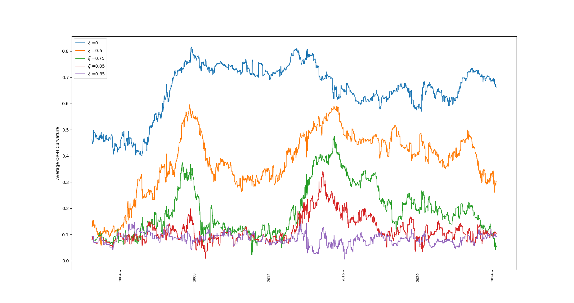
Figures 12, 14, 13 and 15 show that although the general trend is captured by the indicator, changes in $\xi$ are extremely significant for short-period analysis.

Next, we show the same behaviour is observed in the noisy case (arguably the case of most interest) corresponding to smaller values of $T$.

We continue the same simulations for $T=132$ in order to show that the phenomena explained in the previous section prevails in a slightly smoother case.

In this section we choose companies from the S&P ETFs for Canadian companies and evaluate the $\operatorname{O-Ricci}$ estimator.

Figure 23 shows the relative difference (according to $\operatorname{O-Ricci}^{net}$) of the financial crisis of 2008 and the impact of the Covid-19 pandemic on $\operatorname{O-Ricci}^{net}$. From 23 we see that the impact of the 2008 crisis on correlations of the stock market is higher than that of the pandemic. In the following figure (Figure 24) we see this difference replicated for most values of $\xi$, making the analysis much more robust.

From the sub-graph of the Canadian market with large $T$ (Figures 25(c) and 25(d)), we observe a clear increase in fragility during 2004-2008 period and a clear decrease in the indicator for all values of $\xi$ in 2018-2020, followed by another increase at the same time as the Covid-19 pandemic.

In this section we look at the $\operatorname{O-Ricci}$ curvature of a specific subgraph of the market. We look at the technology sector in order to analyze it’s fragility before the famous Tech crunch resulting in the lay-offs of 2023-2024. As before, for values of $\xi\in(0.75,0.85)$ the plot seems more stable. Nevertheless, the indicator does not show the fragility of the sector in a predictive manner (one possible explanation for the decrease in curvature are the lay-offs themselves). We use the time period 2018-2024 instead of 1997-2024 as most current tech companies have had their IPOs in more recent times.

Figure 28 shows the complexity of choosing the parameters for the indicator. While we expect large $T$ ($2000$) to show a clearer picture, for the Tech Industry it seems to be “too big”. In the $T=2000$ case different values of $xi$ show different behaviours, while $T=132$ successfully captures some peaks for most values of $\xi$. One possible explanation for this phenomena is that this sector is deemed to be more volatile, in some underlying sense, so large values of $T$ “average out” the local tendencies.

As argued in Section 3.1, the $\operatorname{O-Ricci}$ curvature of the MST seems to have no direct relation to the $\operatorname{O-Ricci}$ curvature of the original graph. It is reasonable to study a sub-graph which maximizes or minimizes $\operatorname{O-Ricci}^{Net}$. Given a random initial vertex and a size $n$, one can generate a sub0graph with $n$ vertices and minimal $\operatorname{O-Ricci}^{Net}$ following the algorithm in Wu et. al . Whether computing such an indicator performs better than the one presented in Sandhu-Georgiou-Tannenbaum is an interesting open question left for further research (with higher available computational power).

Throughout this work we have shown that $\operatorname{O-Ricci}^{net}$ is a good indicator of crisis periods. The trends in the average Ollivier-Ricci curvature reliably indicate the size and duration of the instability periods of financial markets. For this reason, the indicator can be an important tool for economical and financial analysis.

Due to it’s dependence on the threshold variable $\xi$, as indicated in section 3.5, one should be careful when using $\operatorname{O-Ricci}^{net}$ to predict short time tendencies of the market. In sections 4.2 and 4.3 we observed that the value of $\xi$ the modeller should use depends on the underlying financial market. Thus, it is reasonable to use a Bayesian approach to the determination the threshold. After calibration, $\xi$ should be understood as a hypothesis on which the inference of crisis from $\operatorname{O-Ricci}^{net}$ depends on. As long as this hypothesis is fully assumed, the indicator adds value to our understanding of the random dynamics of financial systems.

Note that Algorithm 2.1 depends on parameters $\xi$ and $D_{i,j}$ together with the use of the MST as the skeleton approach to the underlying network. The use of the MST is currently the most computationally feasible approach to markets with large amounts of data. If the market of interest is of small enough size one can use (1) directly from the constructed network, avoiding having to reduce to the MST and adding links via $\xi$.

One important observation about Algorithm 2.1 is that one should try to avoid dropping incomplete data. Say you want to analyze a market in a period of time where a crash happened, the crash may be a result of subsequent bankruptcy of entities with hidden connections. Computing the indicator after removing such entities misses the dependence on entities which can be fundamental to the crisis. For example, if several banks declare bankruptcy in the time period of study, one does not have complete data after their individual crashes, but it is these crashes that may explain the financial default of the system. Therefore, given a period of time, one should consider every entity which has participated in that period.

In this section we present the lines of investigation which remain open and we believe are of most interest.

References

- (1) S. Miccichè, G. Bonanno, F. Lillo, R. Mantegna, Degree stability of a minimum spanning tree of price return and volatility, Physica A: Statistical Mechanics and its Applications, Volume 324, Issues 1–2,2003,Pages 66-73.
- (2) V. Boginski, S. Butenko, P. M. Pardalos, Mining market data: A network approach., Comput. Oper. Res. 33, 3171–3184 (2006).
- (3) R.J. McCann, Displacement convexity of Boltzmann’s entropy characterizes the strong energy condition from general relativity, Camb. J. Math. 8:3, (2020) 609-681.
- (4) Y. Ollivier, Ricci curvature of metric spaces, C. R. Acad. Sci., Paris, Ser. I 345 (2007) 643–646.
- (5) O.V. Rubleva, The Ricci curvature of a weighted tree, Math Notes, 100, 597–606 (2016). https://doi.org/10.1134/S0001434616090315
- (6) A. Samal , H. Pharasi, J.S. Ramaia, H. Kannan, E. Saucan, J. Jost, A. Chakraborti Network geometry and market instability R. Soc. Open Sci. 8201734 2021
- (7) R. Sandhu , T. T. Georgiou, A.R. Tannenbaum, Ricci curvature: An economic indicator for market fragility and systemic risk, Sci. Adv.2, e1501495, (2016).
- (8) F. Santambrogio, Optimal Transport for Applied Mathematicians Calculus of Variations, PDEs, and Modeling, Progress in Nonlinear Differential Equations and Their Applications (PNLDE, volume 87), Springer.
- (9) C. K. Tse, J. Liu, F. C. M. Lau, A network perspective of the stock market., J. Empir. Financ. 17, 659–667 (2010).
- (10) C. Villani, Optimal Transport: Old and New, Springer, A series of Comprehensive Studies in Mathematics, 2009, Berlin.
- (11) S. Wu, H. Cheng, J. Cai, P. Ma, w.Zhong, Subsampling in Large Graphs Using Ricci Curvature, The Eleventh International Conference on Learning Representations , 2023.
- (12) X-G. Yan, C. Xie, G-J Wang, Stock market network’s topological stability: Evidence from planar maximally filtered graph and minimal spanning tree, International Journal of Modern Physics B, 29,22, Pg.155-161,2015.