On the nonlinear stochastic dynamics of a continuous system with discrete attached elements

Americo Cunha Jr [email protected] Rubens Sampaio [email protected] Department of Mechanical Engineering, PUC–Rio
Rua Marquês de São Vicente, 225, Gávea, Rio de Janeiro - RJ, Brazil - 22453-900

Abstract

This paper presents a theoretical study on the influence of a discrete element in the nonlinear dynamics of a continuous mechanical system subject to randomness in the model parameters. This system is composed by an elastic bar, attached to springs and a lumped mass, with a random elastic modulus and subjected to a Gaussian white-noise distributed external force. One can note that the dynamic behavior of the bar is significantly altered when the lumped mass is varied, becoming, on the right extreme and for large values of the concentrated mass, similar to a mass-spring system. It is also observed that the system response is more influenced by the randomness for small values of the lumped mass. The study conducted also show an irregular distribution of energy through the spectrum of frequencies, asymmetries and multimodal behavior in the probability distributions of the lumped mass velocity.

keywords:

nonlinear dynamics; stochastic modeling; parametric probabilistic approach; uncertainty quantification; maximum entropy principle; Monte Carlo method

^†^†journal: Applied Mathematical Modelling

1 Introduction

A couple of engineering structure has small parts whose dimensions are negligible compared to the entire structure, but its presence induces significant effects on its behavior. In this situation it is common to model the structure as a continuous system with discrete elements coupled. The open literature reports studies that use such continuous/discrete models for the analysis of drillstrings [20], carbon nanotubes [3, 18], naval structure-motor coupling [22], beams coupled with springs [13, 17], a damper [14] and/or a discrete mass [2], etc.

Like any computational model, these continuous/discrete models are subjected to uncertainties. These uncertainties are due to the variability of the model parameters (physical constants, geometry, etc), and mainly due to the possible inaccuracies committed in the model conception (wrong hypotheses about the physics) [23, 24, 25].

In this sense, this work intends to analyze the influence of discrete elements in a continuous mechanical system subjected to randomness in the model parameters. For this, it is considered a one-dimensional elastic bar, with random elastic modulus, fixed on the left extreme and with a lumped mass and two springs (one linear and another nonlinear) on the right extreme, with viscous damping, and subjected to an external force which is proportional to a Gaussian white-noise. The theoretical study developed aims to illustrate a consistent methodology to analyze the influence of coupled discrete elements into the stochastic dynamics of nonlinear mechanical systems. The results of this study complement a series of preliminary studies made on the same subject [8, 9, 10, 11].

The work is organized as follows. The section 2 presents the deterministic equation of the model, its variational form, and the discretization procedure used to solve it. The stochastic modeling of the problem is shown in section 3, as well as the construction of a probability distribution for the elastic modulus, using the maximum entropy principle. In the section 4, some configurations of the model are analyzed in order to characterize the effect of lumped mass in the nonlinear dynamical system. Finally, in the section 5, the main conclusions are emphasized.

2 Deterministic modeling of the mechanical system

2.1 Strong form of the initial–boundary value problem

The mechanical system that will be studied in this work is presented Figure 1. It consists of an elastic bar for which the left side is fixed at a rigid wall, and the right side is attached to a lumped mass and two springs (one linear and one nonlinear). For simplicity, from now on, this system will be called the fixed-mass-spring bar or simply the bar.

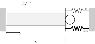
Refer to caption — Figure 1: Sketch of a bar fixed at one end, and attached to two springs and a lumped mass on the other extreme.

The bar displacement field¹¹1The field $\displaystyle u$ is implicitly assumed to be as regular as needed for the initial–boundary value problem of Eqs.(2.1) to (3) to be well posed. $\displaystyle u$ , which depends on the position $\displaystyle x$ and the time $\displaystyle t$ , evolves, for all $\displaystyle(x,t)\in(0,L)\times(t_{0},t_{f}]$ , according to

	$\displaystyle\displaystyle\rho A\mathinner{\dfrac{\partial{{}^{2}}u}{\partial{t^{2}}}}+c\mathinner{\dfrac{\partial{}u}{\partial{t}}}$	$\displaystyle\displaystyle=$	$\displaystyle\displaystyle\mathinner{\dfrac{\partial{}}{\partial{x}}}\left(EA\mathinner{\dfrac{\partial{}u}{\partial{x}}}\right)$
		$\displaystyle\displaystyle-$	$\displaystyle\displaystyle\left(ku+k_{NL}u^{3}+m\mathinner{\dfrac{\partial{{}^{2}}u}{\partial{t^{2}}}}\right)\delta(x-L)+f(x,t),$

where $\displaystyle\rho$ is mass density, $\displaystyle A$ is the cross section area, $\displaystyle c$ is the damping coefficient, $\displaystyle E$ is the elastic modulus, $\displaystyle k$ is the stiffness of the linear spring, $\displaystyle k_{NL}$ is the stiffness of the nonlinear spring, $\displaystyle m$ is the lumped mass, and $\displaystyle f$ is a distributed external force, which depends on $\displaystyle x$ and $\displaystyle t$ . The symbol $\displaystyle\delta(x-L)$ denotes the delta of Dirac distribution at $\displaystyle x=L$ , where $\displaystyle L$ is the bar length.

The boundary conditions for this problem are given by

u(0,t)=0,\leavevmode\nobreak\ \leavevmode\nobreak\ \mbox{and}\leavevmode\nobreak\ \leavevmode\nobreak\ EA\mathinner{\dfrac{\partial{}u}{\partial{x}}}(L,t)=0,

(2)

and the initial position and the initial velocity of the bar are

u(x,t_{0})=u_{0}(x),\leavevmode\nobreak\ \leavevmode\nobreak\ \mbox{and}\leavevmode\nobreak\ \leavevmode\nobreak\ \mathinner{\dfrac{\partial{}u}{\partial{t}}}(x,t_{0})=v_{0}(x),

(3)

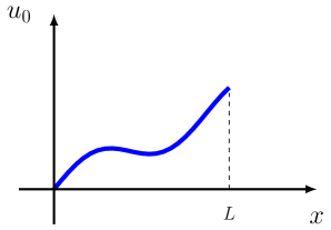
$\displaystyle u_{0}$ and $\displaystyle v_{0}$ being known functions of $\displaystyle x$ , defined for $\displaystyle 0\leq x\leq L$ . For instance,

u_{0}(x)=\alpha_{1}\phi_{3}(x)+\alpha_{2}x,\leavevmode\nobreak\ \leavevmode\nobreak\ \mbox{and}\leavevmode\nobreak\ \leavevmode\nobreak\ v_{0}(x)=0,

(4)

where $\displaystyle\alpha_{1}$ and $\displaystyle\alpha_{2}$ are constants, and $\displaystyle\phi_{3}$ is the third mode²²2Further details in the section 2.4 of the bar. Note that $\displaystyle u_{0}$ reaches the maximum value at $\displaystyle x=L$ , see Figure 2 for instance. This function is used to “activate” the spring cubic nonlinearity, which depends on the displacement at $\displaystyle x=L$ .

2.2 Weak form of the initial–boundary value problem

Let $\displaystyle\mathcal{U}_{t}$ be a class of (time dependent) basis functions and $\displaystyle\mathcal{W}$ be a class of weight functions. These sets are chosen as the space of functions with square integrable spatial derivative, which satisfy the essential boundary condition defined by Eq.(2).

The weak formulation of the initial–boundary value problem above consists in finding, for all $\displaystyle w$ in $\displaystyle\mathcal{W}$ , a displacement field $\displaystyle u$ in $\displaystyle\mathcal{U}_{t}$ such that the following equations are satisfied

\mathcal{M}(\ddot{u},w)+\mathcal{C}(\dot{u},w)+\mathcal{K}(u,w)=\mathcal{F}(w)+\mathcal{F}_{NL}(u,w),

(5)

\widetilde{\mathcal{M}}(u(\cdot,t_{0}),w)=\widetilde{\mathcal{M}}(u_{0},w),

(6)

and

\widetilde{\mathcal{M}}(\dot{u}(\cdot,t_{0}),w)=\widetilde{\mathcal{M}}(v_{0},w),

(7)

where $\displaystyle\mathcal{M}$ is the mass operator, $\displaystyle\mathcal{C}$ is the damping operator, $\displaystyle\mathcal{K}$ is the stiffness operator, $\displaystyle\mathcal{F}$ is the distributed external force operator, $\displaystyle\mathcal{F}_{NL}$ is the nonlinear force operator, and $\displaystyle\widetilde{\mathcal{M}}$ is the associated mass operator. These operators are, respectively, defined as

$\displaystyle\displaystyle\mathcal{M}(\ddot{u},w)$	$\displaystyle\displaystyle=$	$\displaystyle\displaystyle\int_{0}^{L}\rho\,A\,\ddot{u}(x,t)\,w(x)\,dx+m\,\ddot{u}(L,t)\,w(L),$	(8)
$\displaystyle\displaystyle\mathcal{C}(\dot{u},w)$	$\displaystyle\displaystyle=$	$\displaystyle\displaystyle\int_{0}^{L}c\,\dot{u}(x,t)\,w(x)\,dx,$	(9)
$\displaystyle\displaystyle\mathcal{K}(u,w)$	$\displaystyle\displaystyle=$	$\displaystyle\displaystyle\int_{0}^{L}E\,A\,u^{\prime}(x,t)\,w^{\prime}(x)\,dx+k\,u(L,t)\,w(L),$	(10)
$\displaystyle\displaystyle\mathcal{F}(w)$	$\displaystyle\displaystyle=$	$\displaystyle\displaystyle\int_{0}^{L}f(x,t)\,w(x)\,dx,$	(11)
$\displaystyle\displaystyle\mathcal{F}_{NL}(u,w)$	$\displaystyle\displaystyle=$	$\displaystyle\displaystyle-k_{NL}\,\left(u(L,t)\right)^{3}w(L),$	(12)
$\displaystyle\displaystyle\widetilde{\mathcal{M}}(u,w)$	$\displaystyle\displaystyle=$	$\displaystyle\displaystyle\int_{0}^{L}\rho\,A\,u(x,t)\,w(x)\,dx,$	(13)

where $\displaystyle\dot{}$ is an abbreviation for time derivative and ^′ is an abbreviation for spatial derivative.

2.3 Linear conservative dynamics associated

Consider the linear homogeneous equation associated to the Eq.(5),

\mathcal{M}(u,w)+\mathcal{K}(u,w)=0,

(14)

obtained when disposing the dissipation and the external forces acting on the mechanical system.

Assume that Eq.(14) has a solution of the form $\displaystyle u(x,t)=e^{i\nu t}\phi(x)$ , where $\displaystyle\nu$ is the natural frequency, $\displaystyle\phi$ is mode and $\displaystyle i=\sqrt{-1}$ is the imaginary unit. Replacing this expression of $\displaystyle u$ in the Eq.(14), and using the linearity of the operators $\displaystyle\mathcal{M}$ and $\displaystyle\mathcal{K}$ , one gets

\left(-\nu^{2}\mathcal{M}(\phi,w)+\mathcal{K}(\phi,w)\right)e^{i\nu t}=0,

(15)

which, since $\displaystyle e^{i\nu t}\neq 0$ for all $\displaystyle t$ , is equivalent to

-\nu^{2}\mathcal{M}(\phi,w)+\mathcal{K}(\phi,w)=0,

(16)

a generalized eigenvalue problem.

In order to solve the generalized eigenvalue problem defined by Eq.(16), the technique of separation of variables is employed, which leads to a Sturm-Liouville problem [1], with denumerable number of solutions. Therefore, this problem has a denumerable number of solutions, all of then such as the following eigenpair $\displaystyle(\nu_{n}^{2},\phi_{n})$ , where $\displaystyle\nu_{n}$ is the $\displaystyle n$ -th natural frequency and $\displaystyle\phi_{n}$ is the $\displaystyle n$ -th mode of the system.

Note that, the eigenfunctions $\displaystyle\{\phi_{n}\}_{n=1}^{+\infty}$ span the space of functions which contains the solution of the Eq.(16) [6]. Also, as can be seen in [15], these eigenfunctions satisfy, for all $\displaystyle m\neq n$ , the orthogonality relations given by

\mathcal{M}(\phi_{n},\phi_{m})=0,

(17)

and

\mathcal{K}(\phi_{n},\phi_{m})=0.

(18)

The characteristics listed above made the modes of the system good choices for the basis function, when one uses a weighted residual procedure [12] to approximate the solution of the nonlinear variational problem defined by Eqs.(5) to (7).

2.4 Modes and natural frequencies

According to [4], a fixed-mass-spring bar has its natural frequencies and the corresponding orthogonal modes shape given by

\nu_{n}=\lambda_{n}\frac{\bar{c}}{L},

(19)

and

\phi_{n}(x)=\sin{\left(\lambda_{n}\frac{x}{L}\right)},

(20)

where $\displaystyle\bar{c}=\sqrt{E/\rho}$ is the wave speed, and the $\displaystyle\lambda_{n}$ are the solutions of

\cot{\left(\lambda_{n}\right)}+\left(\frac{kL}{AE}\right)\frac{1}{\lambda_{n}}-\left(\frac{m}{\rho AL}\right)\lambda_{n}=0.

(21)

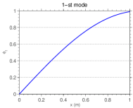
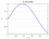
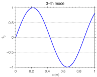
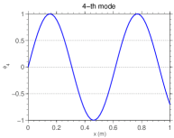
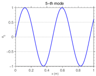
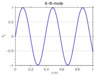
The first six orthogonal modes shape of the fixed-mass-spring bar with $\displaystyle m=1.5\leavevmode\nobreak\ kg$ , whose the other parameters are presented in the beginning of section 4, are illustrated in Figure 3. In this figure each sub-caption indicates the approximated natural frequency associated with the corresponding mode.

2.5 Discretization of the model equations

The Galerkin method [16] is employed to approximates the solution of the variational problem given by Eqs.(5) to (7). In this weighted residual procedure the displacement field $\displaystyle u$ is approximated as

u(x,t)\approx\sum_{n=1}^{N}u_{n}(t)\phi_{n}(x),

(22)

where the basis functions $\displaystyle\phi_{n}$ are the orthogonal modes of the conservative and non-forced dynamical system associated to the fixed-mass-spring bar, and the coefficients $\displaystyle u_{n}$ are time-dependent functions. This results in the following system of nonlinear ordinary differential equations

\left[M\right]\ddot{\mathbf{u}}(t)+\left[C\right]\dot{\mathbf{u}}(t)+\left[K\right]\mathbf{u}(t)=\mathbf{f}(t)+\mathbf{f}_{NL}\left(\dot{\mathbf{u}}(t)\right),

(23)

supplemented by the following pair of initial conditions

\mathbf{u}(t_{0})=\mathbf{u}_{0}\qquad\mbox{and}\qquad\mathbf{\dot{u}}(t_{0})=\mathbf{v}_{0},

(24)

where $\displaystyle\mathbf{u}(t)$ is the vector of $\displaystyle\mathbb{R}^{N}$ in which the $\displaystyle n$ -th component is $\displaystyle u_{n}(t)$ , $\displaystyle\left[M\right]$ is the mass matrix, $\displaystyle\left[C\right]$ is the damping matrix, $\displaystyle\left[K\right]$ is the stiffness matrix. Also, $\displaystyle\mathbf{f}(t)$ , $\displaystyle\mathbf{f}_{NL}\left(\mathbf{u}(t)\right)$ , $\displaystyle\mathbf{u}_{0}$ , and $\displaystyle\mathbf{v}_{0}$ are vectors of $\displaystyle\mathbb{R}^{N}$ , which respectively represent the external force, the nonlinear force, the initial position, and the initial velocity. The initial value problem of Eqs.(23) and (24) has its solution approximated by Newmark method [16], in which a Newton-Raphson iteration is used to solve the nonlinear system of algebraic equations that arises from the discretization.

3 Stochastic modeling of the mechanical system

3.1 Stochastic initial–boundary value problem

Consider a probability space $\displaystyle(\SS,{\mathbb{A}},{\mathbb{P}})$ , where $\displaystyle\SS$ is sample space, $\displaystyle{\mathbb{A}}$ is a $\displaystyle\sigma$ -field over $\displaystyle\SS$ and $\displaystyle{\mathbb{P}}$ is a probability measure. In this probability space, the elastic modulus is assumed to be a random variable $\displaystyle E\mathrel{\mathop{\mathchar 58\relax}}\SS\to\mathbb{R}$ , and the distributed external force a random field $\displaystyle F\mathrel{\mathop{\mathchar 58\relax}}[0,L]\times[t_{0},t_{f}]\times\SS\to\mathbb{R}$ .

Due to the randomness of $\displaystyle F$ and $\displaystyle E$ , the bar displacement becomes a random field $\displaystyle U\mathrel{\mathop{\mathchar 58\relax}}[0,L]\times[t_{0},t_{f}]\times\SS\to\mathbb{R}$ , which evolves according to

	$\displaystyle\displaystyle\rho A\mathinner{\dfrac{\partial{{}^{2}}U}{\partial{t^{2}}}}+c\mathinner{\dfrac{\partial{}U}{\partial{t}}}$	$\displaystyle\displaystyle=$	$\displaystyle\displaystyle\mathinner{\dfrac{\partial{}}{\partial{x}}}\left(EA\mathinner{\dfrac{\partial{}U}{\partial{x}}}\right)$
		$\displaystyle\displaystyle-$	$\displaystyle\displaystyle\left(kU+k_{NL}U^{3}+m\mathinner{\dfrac{\partial{{}^{2}}U}{\partial{t^{2}}}}\right)\delta(x-L)+F(x,t,\theta).$

This problem has boundary and initial conditions similar to those defined in Eqs.(2) and (3), by changing $\displaystyle u$ for $\displaystyle U$ only. Furthermore, the partial derivatives now are not defined in the classical way, but in the mean square sense [19].

3.2 Random external force modeling

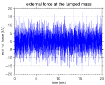
The distributed external force acting on the bar is assumed as the form

F(x,t,\theta)=\sigma\phi_{1}(x)N(t,\theta),

(26)

where $\displaystyle\sigma$ is the force amplitude, $\displaystyle\phi_{1}$ the bar first mode³³3The choice of the spatial shape of the excitation seek for a configuration that is physically plausible and simple. The first mode meets both requirements., and $\displaystyle N(t,\theta)$ is a Gaussian white-noise⁴⁴4Remember that a white-noise is a random process which all instants of time are uncorrelated. In other words, the behavior of the process at any given instant of time has no influence on the other instants. with zero mean and unit variance.

A typical realization of the random external force, given by Eq.(26), for fixed position, is shown in Figure 4.

3.3 Random elastic modulus distribution

The elastic modulus cannot be negative, so it is reasonable to assume the support of $\displaystyle E$ as the interval $\displaystyle(0,\infty)$ . Therefore, the probability density function (PDF) of $\displaystyle E$ is a nonnegative function $\displaystyle p_{\tiny{E}}\mathrel{\mathop{\mathchar 58\relax}}(0,\infty)\to\mathbb{R}$ , which respects the following normalization condition

\int_{0}^{\infty}p_{\tiny{E}}(\xi)\,d\xi=1.

(27)

Additionally, it is supposed that the expected value of $\displaystyle E$ is a known (finite) real number, i.e.,

\int_{0}^{\infty}E(\xi)\,p_{\tiny{E}}(\xi)\,d\xi=\mu_{E}<\infty,

(28)

as well as the expected value of $\displaystyle\ln{\left(E\right)}$ ,

\int_{0}^{\infty}\ln{\left(E\right)}\,p_{\tiny{E}}(\xi)\,d\xi=\mu_{\ln{\left(E\right)}}<\infty,

(29)

being the latter requirement a sufficient condition to ensure that $\displaystyle E^{-1}$ exists almost sure, and is a second order random variable [23, 24].

Following the suggestion of [23, 24, 25], the maximum entropy principle is employed in order to consistently specify $\displaystyle p_{\tiny{E}}$ . This methodology chooses for $\displaystyle E$ the PDF which maximizes the entropy function defined by

\mathbb{S}\left[p_{\tiny{E}}\right]=-\int_{0}^{\infty}p_{\tiny{E}}(\xi)\,\ln\left(p_{\tiny{E}}(\xi)\right)\,d\xi,

(30)

subjected to the constraints given by (27), (28) and (29). These restrictions effectively define the known information about $\displaystyle E$ .

The gamma distribution is the one which solves the optimization problem above, and its PDF is given by

p_{\tiny{E}}(\xi)=\mathds{1}_{(0,\infty)}\frac{1}{\mu_{E}}\left(\frac{1}{\delta_{E}^{2}}\right)^{\left(\displaystyle\frac{1}{\delta_{E}^{2}}\right)}\frac{1}{\Gamma(1/\delta_{E}^{2})}\left(\frac{\xi}{\mu_{E}}\right)^{\left(\displaystyle\frac{1}{\delta_{E}^{2}}-1\right)}\exp\left(-\frac{\xi}{\delta_{E}^{2}\mu_{E}}\right),

(31)

where $\displaystyle\mathds{1}_{(0,\infty)}$ denotes the indicator function of the interval $\displaystyle(0,\infty)$ , $\displaystyle\Gamma$ indicates the gamma function, and $\displaystyle\delta_{E}$ is a type of dispersion parameter, such that $\displaystyle 1\leq\delta_{E}\leq 1/\sqrt{2}$ , defined as the ratio between the standard deviation and the mean of $\displaystyle E$ .

3.4 Stochastic solver: Monte Carlo method

Uncertainty propagation in the nonlinear stochastic dynamics of the bar is computed by Monte Carlo (MC) method [21, 7]. This stochastic solver uses a pseudorandom number generator to obtain many realizations of $\displaystyle E$ and $\displaystyle F$ . Each one of these realizations defines a new Eq.(5), so that a new weak problem is obtained. After that, these new weak problems are solved deterministically, such as in section 2.5. All the MC simulations reported in this work use $\displaystyle 4096$ samples to access the random system.

4 Numerical experimentation

The numerical experiments presented in this section adopt for the system parameters the deterministic values shown in Table 1. Also, the random variable $\displaystyle E$ , is characterized by the mean $\displaystyle\mu_{E}=203\leavevmode\nobreak\ GPa$ and the dispersion $\displaystyle\delta_{E}=0.1$ .

Table 1: This table presents the deterministic (nominal) parameters used in the numerical simulations reported in this work.

parameter	value	unit
$\displaystyle\rho$	$\displaystyle 7900$	$\displaystyle kg/m^{3}$
$\displaystyle A$	$\displaystyle 625\pi$	$\displaystyle mm^{2}$
$\displaystyle L$	$\displaystyle 1$	$\displaystyle m$
$\displaystyle c$	$\displaystyle 5$	$\displaystyle kN/s$
$\displaystyle k$	$\displaystyle 650$	$\displaystyle N/m$
$\displaystyle k_{NL}$	$\displaystyle 650\times 10^{13}$	$\displaystyle N/m^{3}$
$\displaystyle\sigma$	$\displaystyle 5$	$\displaystyle kN$
$\displaystyle\alpha_{1}$	$\displaystyle 0.1$	$\displaystyle mm$
$\displaystyle\alpha_{2}$	$\displaystyle 0.5\times 10^{-3}$	—

The approximation to the solution of the weak initial-boundary value problem of section 2.2, constructed as described in the section 2.5, uses 10 modes. As the 10-th natural frequency of the system is $\displaystyle\approx 23.08\leavevmode\nobreak\ kHz$ , a representative frequency band of this dynamical system is $\displaystyle\mathfrak{B}=[0,25]\leavevmode\nobreak\ kHz$ . Thus, to analyze the dynamics of the system in this frequency band, it is adopted a “temporal window” given by the interval $\displaystyle[t_{0},t_{f}]=[0,20]\leavevmode\nobreak\ ms$ .

For sake of reference, a deterministic (nominal) model, with $\displaystyle E=\mu_{E}$ , and $\displaystyle f(x,t)=\sigma\phi_{1}(x)$ , is considered. Furthermore, a parametric study, with $\displaystyle m^{\ast}=0.1,\leavevmode\nobreak\ 1,\leavevmode\nobreak\ 10,\leavevmode\nobreak\ 50$ , is performed to investigate the effect of the end mass on the bar dynamics, where the discrete–continuous mass ratio is defined as

m^{\ast}=\frac{m}{\rho AL}.

(32)

4.1 Evolution of the lumped mass velocity

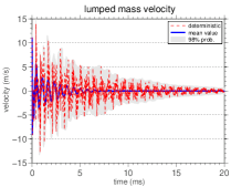
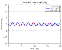
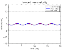
The mean value of the lumped mass velocity, i.e, $\displaystyle\dot{U}(L,\cdot,\cdot)$ , its nominal value, and an envelope of reliability, wherein a realization of the stochastic system has 98% of probability of being contained, are shown, for different values of $\displaystyle m^{\ast}$ , in Figure 5. By observing this figure one can note that, as the value of lumped mass increases, the mean value tends to the nominal value. That is, the system is “more random” for small values of $\displaystyle m^{\ast}$ .

Also, the analysis of Figure 5 shows that, for large values of $\displaystyle m^{\ast}$ , the decay in the system displacement amplitude decreases significantly, i.e., the system is not much influenced by damping as $\displaystyle m^{\ast}\to\infty$ .

Explanations for the observations made in the preceding paragraphs of this section are provided by the analysis of the system orbit in phase space, which is done in the section 4.2.

Furthermore, the amplitude of the confidence interval increases with time for all values of $\displaystyle m^{\ast}$ , i.e., the system uncertainty at $\displaystyle x=L$ is greater in the stationary regime. This is evident in the first three graphs, but remains true in the fourth graph, and is due to the accumulation of uncertainties with the increasing time.

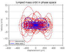
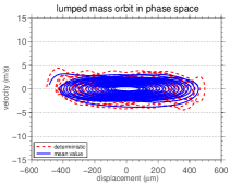
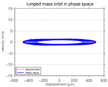
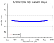
4.2 Orbit of the lumped mass in the mechanical system phase space

The mean orbit, in the phase space, of the fixed-mass-spring bar at $\displaystyle x=L$ is shown, for different values of $\displaystyle m^{\ast}$ , in Figure 6. Distinct behaviors, for the different values of $\displaystyle m^{\ast}$ shown, can be observed.

For $\displaystyle m^{\ast}=0.1$ , the mean orbit is quite different from the “disturbed” nominal orbit observed. This is because the response of the nominal system depends on the initial conditions for a long period, fact which is not observed for the other values of $\displaystyle m^{\ast}$ . This explains why the mean velocity tends to the nominal velocity when $\displaystyle m^{\ast}$ increases.

The assertive made in the second paragraph of section 4.1, about how the influence of the damping in the system decreases, can be confirmed by analyzing the Figure 6, since the mean orbit of the system tends from a stable focus to an ellipse as $\displaystyle m^{\ast}$ increases. So, the limit behavior of the bar right extreme with $\displaystyle m^{\ast}\to\infty$ is a mass-spring system. This limit behavior, which tends to a conservative system, occurs because, with the increasing of $\displaystyle m^{\ast}$ , most of the mass of the system becomes concentrated at the right extreme of the bar. Thus, the bar behaves like a massless spring. Also, as the damping is distributed along the bar and the mass of it became negligible, the viscous dissipation becomes ineffective.

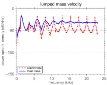
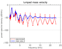
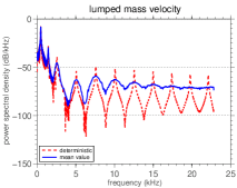
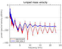
4.3 Power spectral density of the lumped mass velocity

The energy distribution of the bar through the frequency spectrum can be seen in Figure 7, which shows the mean power spectral density (PSD) of the lumped mass (steady state) velocity and its nominal value.

The presence of the white-noise forcing excites the mechanical system in all frequencies of the band $\displaystyle\mathfrak{B}$ . This is made evident by the various peaks in the mean PSD function, each one occurring in a frequency that is very close to a natural frequency of the system. It is important to note that the peaks of the nominal and of the mean PSD occur practically at the same frequencies. Once the forcing does not influence the natural frequencies, the only random parameter to promote changes in natural frequencies is $\displaystyle E$ , whose the randomness is reasonably low.

A larger number of peaks can be seen in the high frequencies, but the peak with greater height, and thus, the more energy, is always the first frequency of the spectrum. As the spatial dependence of the forcing is given by the first mode, as can be seen in Eq.(26), the low frequency of the spectrum receives an “extra contribution” of energy beyond the white-noise.

However, as $\displaystyle m^{\ast}$ increases, the natural frequencies of the associated conservative system decrease, which is not observed in the case of the bar. This difference in the system behavior, as well as irregular redistribution of energy along the spectrum, when $\displaystyle m^{\ast}$ changes, may be due to cubic nonlinearity.

4.4 Probability density function of the lumped mass velocity

The difference between the system dynamical behavior is even clearer if one looks at the PDF estimations⁵⁵5These estimates were obtained using a kernel smooth density technique [5]. of the normalized random variable $\displaystyle\dot{U}(L,t_{f},\cdot)$ , which are presented in Figure 8. Note that in this context normalized means a random variable with zero mean and unit standard deviation.

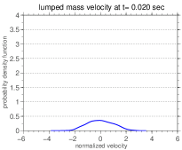
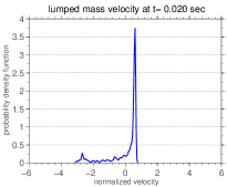
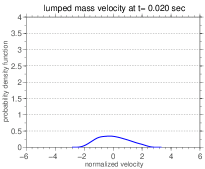
In all cases the PDF presents an asymmetry around the (zero) mean as can be seen in the Table 2, which shows the probability of the normalized random variable $\displaystyle\dot{U}(L,t_{f},\cdot)$ be less than or equal to the mean, for several values of the discrete–continuous mass ratio.

These asymmetries indicate if it is more probable the velocity be higher or lower than the mean, according to the area under the PDF curve to the right or to the left of the mean, respectively. The observed values are in agreement with what is seen in the envelopes of reliability of Figure 5.

Table 2: This table presents the probability of the normalized random variable

\displaystyle\dot{U}(L,t_{f},\cdot)

be less than or equal to the mean, for several values of the discrete–continuous mass ratio.

$\displaystyle m^{\ast}$	probability
0.1	$\displaystyle\thickapprox$ 0.52
1	$\displaystyle\thickapprox$ 0.50
10	$\displaystyle\thickapprox$ 0.28
50	$\displaystyle\thickapprox$ 0.53

Furthermore, it is possible to observe a multimodal behavior in some of the PDFs shown in the Figure 5. This multimodal behavior indicates a high number of realizations close to the values that correspond to the peaks. Therefore, it can be concluded that the regions near the peaks are areas of greater probability for the system response. Note that these areas change irregularly when $\displaystyle m^{\ast}$ is varied.

5 Concluding remarks

This work presents a model to describe the nonlinear dynamics of a elastic bar, attached to discrete elements, with viscous damping, random elastic modulus, and subjected to a Gaussian white-noise distributed external force. The elastic modulus is modeled as a random variable with gamma distribution, being the probability distribution of this parameter obtained by the use of the maximum entropy principle.

An analysis of the model is performed, indexed by a dimensionless parameter which describes the ratio between the discrete/continuous mass of the system. This analysis shows that the dynamics of the random system is significantly altered when the values of the lumped mass are varied. It is observed that this system right extreme behaves, in the limiting case where the lumped mass is very large, such as a mass-spring system. Also, one can note an irregular distribution of energy through the spectrum of frequencies, maybe induced by the cubic nonlinearity. Furthermore, the probability distributions of the lumped mass velocity present asymmetries and multimodal behavior, being this multimodality associated with the existence of areas of greater probability for the dynamic system response.

Acknowledgments

The authors are indebted to the Brazilian agencies CNPq, CAPES, and FAPERJ for the financial support given to this research. They also wish to thank the anonymous referees’, for useful comments and suggestions.

References

Al Gwaiz [2007] Al Gwaiz, M. A., 2007. Sturm-Liouville Theory and its Applications. Springer, New York.
Andrews and Shillor [2002] Andrews, K. T., Shillor, M., 2002. Vibrations of a beam with a damping tip body. Mathematical and Computer Modelling 35 (9–10), 1033–1042.
Aydogdu and Filiz [2011] Aydogdu, M., Filiz, S., 2011. Modeling carbon nanotube-based mass sensors using axial vibration and nonlocal elasticity. Physica E: Low-dimensional Systems and Nanostructures 43, 1229–1234.
Blevins [1993] Blevins, R. D., 1993. Formulas for Natural Frequency and Mode Shape. Krieger Publishing Company, Malabar.
Bowman and Azzalini [1997] Bowman, A. W., Azzalini, A., 1997. Applied Smoothing Techniques for Data Analysis. Oxford University Press, New York.
Brezis [2010] Brezis, H., 2010. Functional Analysis, Sobolev Spaces and Partial Differential Equations. Springer, New York.
Cunha Jr et al. [2014] Cunha Jr, A., Nasser, R., Sampaio, R., Lopes, H., Breitman, K., 2014. Uncertainty quantification through Monte Carlo method in a cloud computing setting. Computer Physics Communications 185, 1355––1363.
Cunha Jr and Sampaio [2012] Cunha Jr, A., Sampaio, R., 2012. Effect of an attached end mass in the dynamics of uncertainty nonlinear continuous random system. Mecánica Computacional 31, 2673–2683.
Cunha Jr and Sampaio [2012] Cunha Jr, A., Sampaio, R., 2012. On the dynamics of a nonlinear continuous random system. In: Proceedings of the 1st International Symposium on Uncertainty Quantification and Stochastic Modeling.
Cunha Jr and Sampaio [2013a] Cunha Jr, A., Sampaio, R., 2013a. Analysis of the nonlinear stochastic dynamics of an elastic bar with an attached end mass. In: Proceedings of the III South-East Conference on Computational Mechanics.
Cunha Jr and Sampaio [2013b] Cunha Jr, A., Sampaio, R., 2013b. Uncertainty propagation in the dynamics of a nonlinear random bar. In: Proceedings of the XV International Symposium on Dynamic Problems of Mechanics.
Finlayson and Scriven [1966] Finlayson, B., Scriven, L., 1966. The method of weighted residuals- A review. Applied Mechanics Reviews 19, 735–748.
Gürgöze and Zeren [2011] Gürgöze, M., Zeren, S., 2011. Consideration of the masses of helical springs in forced vibrations of damped combined systems. Mechanics Research Communications 38, 239–243.
Hagedorn [1987] Hagedorn, P., 1987. Wind-excited vibrations of transmission lines: A comparison of different mathematical models. Mathematical Modelling 8, 352–358.
Hagedorn and DasGupta [2007] Hagedorn, P., DasGupta, A., 2007. Vibrations and Waves in Continuous Mechanical Systems. Wiley, Chichester.
Hughes [2000] Hughes, T. J. R., 2000. The Finite Element Method. Dover Publications, New York.
Mao [2011] Mao, Q., 2011. Free vibration analysis of multiple-stepped beams by using adomian decomposition method. Mathematical and Computer Modelling 54, 756–764.
Murmu and Adhikari [2011] Murmu, T., Adhikari, S., 2011. Nonlocal vibration of carbon nanotubes with attached buckyballs at tip. Mechanics Research Communications 38, 62–67.
Papoulis and Pillai [2002] Papoulis, A., Pillai, S. U., 2002. Probability, Random Variables and Stochastic Processes, 4th Edition. McGraw-Hill, New- York.
Ritto et al. [2013] Ritto, T. G., Escalante, M. R., Sampaio, R., Rosales, M. B., 2013. Drill-string horizontal dynamics with uncertainty on the frictional force. Journal of Sound and Vibration 332, 145–153.
Robert and Casella [2010] Robert, C. P., Casella, G., 2010. Monte Carlo Statistical Methods. Springer, New York.
Rossit and Laura [2001] Rossit, C. A., Laura, P. A. A., 2001. Free vibrations of a cantilever beam with a spring–mass system attached to the free end. Ocean Engineering 28, 933–939.
Soize [2000] Soize, C., 2000. A nonparametric model of random uncertainties for reduced matrix models in structural dynamics. Probabilistic Engineering Mechanics 15, 277 – 294.
Soize [2005] Soize, C., 2005. Random matrix theory for modeling uncertainties in computational mechanics. Computer Methods in Applied Mechanics and Engineering 194, 1333–1366.
Soize [2013] Soize, C., 2013. Stochastic modeling of uncertainties in computational structural dynamics - recent theoretical advances. Journal of Sound and Vibration 332, 2379––2395.