On the missing link between pressure drop, viscous dissipation and the turbulent energy spectrum

For many decades, turbulence has remained stubbornly one of the most challenging open problems in classical physics. Achieving complete understanding of turbulent flows is hindered by the their multi-scale nature, and the complex mechanisms underlying the distribution of energy to the large number of harmonics, which constitute the fluctuating velocity field. It is well accepted that vortex stretching is one of the main mechanisms responsible for transferring energy from low to high wavenumbers. This mechanism, however, only exists in viscous, three-dimensional turbulence, with no analogue in quantum Barenghi et al. (2014), and two-dimensional turbulence Tran et al. (2010).

The pictorial energy cascade proposed by Richardson Richardson (1922), and then recovered theoretically first by Kolmogorov Kolmogorov (1941a, b), and then, independently, by Onsager Eyink and Sreenivasan (2006), does not reveal much about the energy transfer between consecutive harmonics; it only represents an ‘equilibrium’ state of energy distribution arising from a balance between the fluxes of energy going up and down the cascade. Despite the fact that viscous dissipation is irrelevant for quantum turbulence, the scaling laws dominating its energy cascade are the same as those in viscous, three-dimensional turbulence Maurer and Tabeling (1998); Maltrud and Vallis (1991); Smith and Yakhot (1993). What, then, is the true role of viscous dissipation in the formation of the energy cascade, and what is its connection to macroscopic quantities such as the pressure drop? We address the second question in the present letter.

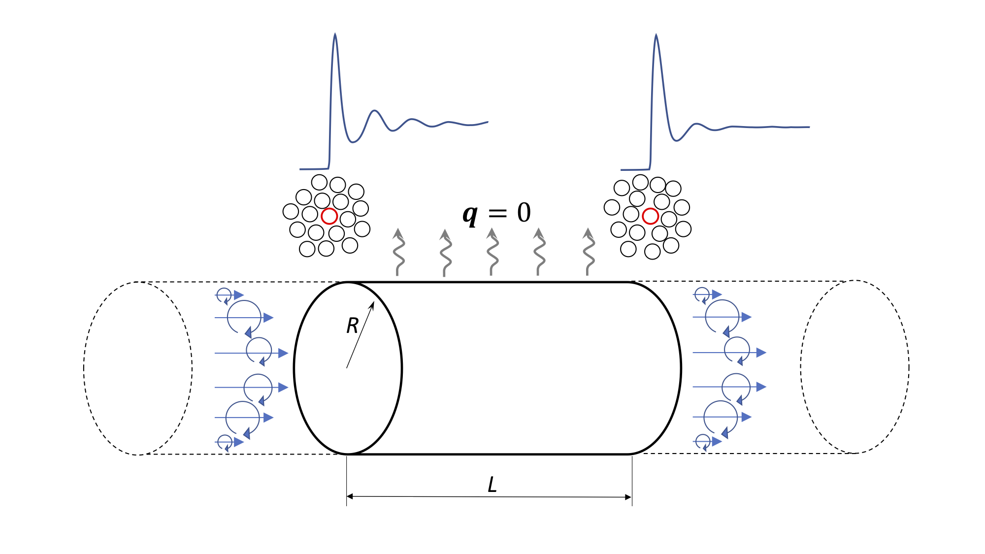
We start our discussion from the conservation of linear momentum $\partial_{t}\textbf{p}+\nabla\cdot\left(\textbf{u}\textbf{p}\right)=-\nabla\cdot\stackrel{{\scriptstyle\leftrightarrow}}{{\bm{\sigma}}}+\Sigma\textbf{f}_{ext}$, with $\textbf{p}=\rho\textbf{u}$ the linear momentum, $\rho$ the density, u the instantaneous velocity field, $\stackrel{{\scriptstyle\leftrightarrow}}{{\bm{\sigma}}}$ the stress tensor, and $\Sigma\textbf{f}_{ext}$ the summation of all external forces. We further split the stress tensor as $\stackrel{{\scriptstyle\leftrightarrow}}{{\bm{\sigma}}}=P\stackrel{{\scriptstyle\leftrightarrow}}{{\textbf{I}}}-\stackrel{{\scriptstyle\leftrightarrow}}{{\bm{\tau}}}$, with $P$ the pressure and $\stackrel{{\scriptstyle\leftrightarrow}}{{\bm{\tau}}}=\mu\left(\nabla\textbf{u}+\nabla\textbf{u}^{T}\right)$ the viscous stress tensor expressed in terms of the dynamic viscosity $\mu$ and the strain rate. In our analysis, we consider a portion of a pipe, where the flow is adiabatic, incompressible and fully developed (Fig. 1). Hence, all the quantities are statistically invariant along the stream-wise direction, except for the fluid pressure.

By applying a time average to the conservation of momentum, we arrive to the following expression for the pressure drop

with $R$ the pipe radius, $L$ the pipe length, $u_{\tau}=\sqrt{\tau_{w}/\rho}$ the friction velocity, $\tau_{w}=\left(\mu\partial U/\partial r\right)_{w}$ the wall shear stress, and $U$ the stream-wise component of the time-averaged velocity field.

An equivalent expression can be obtained from the conservation of kinetic energy $e_{k}=\textbf{u}^{2}/2$ (per unit mass) $\partial_{t}\left(\rho e_{k}\right)+\nabla\cdot\left(\textbf{u}\rho e_{k}+\stackrel{{\scriptstyle\leftrightarrow}}{{\bm{\sigma}}}\cdot\textbf{u}\right)=\stackrel{{\scriptstyle\leftrightarrow}}{{\bm{\sigma}}}\colon\nabla\textbf{u}+\Sigma\textbf{f}_{ext}\cdot\textbf{u}$. By applying a time average to the conservation law for kinetic energy and invoking incompressible and fully developed pipe flow conditions, the pressure drop reads

with $\left\langle\cdot\right\rangle$ a time average, $VA=\int_{A}\textbf{u}\cdot d\textbf{A}$ the volumetric flow rate, $A$ the pipe cross section, and $V$ the average cross section velocity (see supplemental material for a detailed derivation of conservation laws and the two expressions for the pressure drop). Equation (2) was also presented by Pope Pope (2000). Since the conservation law for kinetic energy is not independent from that of momentum, Eqs. (1) and (2) are completely equivalent. Thus, we can express the wall shear stress in terms of the total viscous dissipation.

We need to emphasize that Eq. (3) is only valid for fully developed (laminar or turbulent) and incompressible pipe flow. For laminar flow, it is possible to confirm analytically the validity of Eqs. (2) and (3). The first interesting conclusion from Eq. (2), is that viscous dissipation cannot increase the temperature of a fluid at the incompressibility limit. The conservation of enthalpy per unit mass, $h$, implies that $\rho D_{t}h+\nabla\cdot\textbf{q}=D_{t}P+\stackrel{{\scriptstyle\leftrightarrow}}{{\bm{\tau}}}\colon\nabla\textbf{u}$ (see supplemental material), with $D_{t}=\partial_{t}+\textbf{u}\cdot\nabla$ the material derivative and q the heat flux. If the pipe is adiabatic and the flow incompressible, the only possibility for the enthalpy to change, is through viscous heating (dissipation term). After applying a time average to the conservation law of enthalpy, the integration of the R.H.S. over the pipe volume, vanishes by virtue of Eq. (2) and, thus, $\int_{\Omega}\left\langle\rho D_{t}h\right\rangle d\Omega=0$. Since there is no energy exchange with the environment (adiabatic flow), this requires either a constant fluid temperature or that the local viscous dissipation increase and decrease the local fluid temperature in a way that the net change of total enthalpy is null. Because the second option would be in violation with the first law of thermodynamics, the fluid temperature must be constant at the incompressibility limit.

For molecular fluids like water, the internal energy can suffer important variations by changing the molecular arrangement, keeping an almost constant temperature and density. A small change in the enthalpy per unit volume, $\tilde{h}$, is given by $d\tilde{h}=de_{u}+dP$, with $e_{u}$ being the internal energy per unit volume. If the enthalpy of the fluid is constant, then $de_{u}/dP=-1$. Molecular Dynamics (MD) simulations of water at constant temperature Mahoney and Jorgensen (2000), indicate that the local range order (a measure of how molecules are arranged in the liquid) undergoes important changes as pressure increases. Using the MD data from Mahoney and Jorgensen Mahoney and Jorgensen (2000), we can estimate the derivative $de_{u}/dP$. Applying a linear fit to their MD data yields a value of $de_{u}/dP\sim-0.826$ (see supplemental material). Since the fluid considered in the MD study is slightly compressible Mahoney and Jorgensen (2000), we would expect a value slightly different from $-1$. These molecular studies, show the strong degree of correlation between internal energy and the molecular arrangement of the liquid. This would imply that for strictly incompressible fluids, the energy of the flow (pressure + kinetic) is dissipated only into the potential component of the internal energy following a reversible path, and not, as commonly believed, into the micro-kinetic component of the internal energy (temperature). For a liquid flowing in a pipe, the higher pressure at the inlet will cause a slightly higher degree of molecular order compared to that at the outlet (see Fig. 1).

To reveal the connection between Eq. (2) and the turbulent the energy spectrum, we follow the work of Gioia and ChakrabortyGioia and Chakraborty (2006). They investigated the relationship between the friction factor, $f=8\tau_{w}/\rho V^{2}$ and the phenomenological turbulent energy spectrum. Considering the Darcy-Weisbach equation, we can express the pressure drop as

where $D_{H}$ the hydraulic pipe diameter. The negative sign is to enforce a decrease in the pressure along the pipe. By replacing Eq. (2) into (4) and introducing the Reynolds decomposition $\textbf{u}=\textbf{U}+\textbf{u}^{\prime}$, with $\textbf{U}=\left\langle\textbf{u}\right\rangle$, we can express the friction factor in terms of two components of the viscous dissipation,

where $\nu$ is the kinematic viscosity, and $\rho^{-1}\left\langle\stackrel{{\scriptstyle\leftrightarrow}}{{\bm{\tau}}}\colon\nabla\textbf{u}\right\rangle=\overline{\epsilon_{0}}+\epsilon_{0}^{\prime}$ is defined as the total time-averaged dissipation, with $\overline{\epsilon_{0}}/\nu=\nabla\textbf{U}\colon\nabla\textbf{U}+\nabla\textbf{U}^{T}\colon\nabla\textbf{U}$ and $\epsilon_{0}^{\prime}/\nu=\left\langle\nabla\textbf{u}^{\prime}\colon\nabla\textbf{u}^{\prime}+\nabla\textbf{u}^{\prime T}\colon\nabla\textbf{u}^{\prime}\right\rangle$ the mean and turbulent components of the viscous dissipation respectively. The Reynolds number, $\mbox{{Re}}=VD_{H}/\nu$, is defined in terms of the hydraulic pipe diameter, $D_{H}$ .

The main difficulty faced by Gioia and Chakraborty Gioia and Chakraborty (2006), was the determination of the wall shear stress, and how to relate it to the turbulent energy spectrum and the surface roughness. They postulated that the wall shear stress can be expressed in terms of a momentum transfer between the bulk flow and the flow near the wall, characterized by a velocity scale $u_{s}$. Expressing the wall stress as $\tau_{w}=\rho Vu_{s}$, the problem reduces to finding the velocity scale, which might also vary with the amplitude of the surface roughness. Furthermore, to determine the velocity scale they assumed the validity of the phenomenological energy spectrum in the proximity of the wall, which is something arguable. It is well known, however, that to derive the phenomenological spectrum, the turbulent structures must be rotationally- and translationally-invariant; that is, the flow is isotropic and homogenous, which is not the case near the wall. Aware of this limitation, Gioia and ChakrabortyGioia and Chakraborty (2006) argue that even for anisotropic and inhomogeneous flows, the phenomenological theory still represents a good approximation. Thus, by using directly the energy spectrum $E\left(q\right)$ (including corrections for the energetic and dissipative ranges), they obtain the velocity scale as $u_{s}^{2}=\int_{1/s}^{\infty}{E\left(q\right)}dq$. Here, the integration is carried out for wave numbers higher than $1/s=1/\left(r+a\eta\right)$, where $a$ is a dimensionless constant, $r$ the size of the surface roughness, and $\eta$ the Kolmogorov length scale. Hence, they are effectively filtering out all eddies larger than $s$ in the calculation of the velocity scale. It is remarkable that for $\mbox{{Re}}\rightarrow\infty$, the friction factor in the work of Gioia and ChakrabortyGioia and Chakraborty (2006) scales as $f\sim(r/R)^{1/3}$ despite the absence of a correction for the dissipative regime, $C_{d}\left(q\right)$, in the turbulent energy spectrum: without this, the total dissipation diverges when using the Kolmogorov spectrum. The authors recovered the proper scaling for the friction factor, observed in Nikuradse’s experimental results, only by selecting an appropriate cutoff wave length ($1/s$) in the integration of the energy spectrum.

To avoid an arbitrary selection of the cutoff wave length, we follow a different route. In our analysis, we start by investigating the direct connection between the friction factor, defined in Eq. (S28) with the turbulent energy spectrum. Considering an spherically and volumetric averaged spectrum $\hat{R}_{0}$ (see details in the supplemental material), along with Taylor’s identities for isotropic turbulenceTaylor (1935), we can approximate the total viscous dissipation by $\epsilon^{\prime}_{0}\approx 15\nu\int_{0}^{\infty}q^{2}\hat{R}_{0}dq$. It is noteworthy to mention that in our analysis, $\hat{R}_{0}$, does not correspond to the spectrum of any particular point inside the pipe, but rather an averaged quantity. We now analyze the asymptotic behavior of Eq. (S28). For $\mbox{{Re}}\rightarrow 0$, $\int_{\Omega}\overline{\epsilon}_{0}/\nu d\Omega\rightarrow 8\pi LV^{2}$ and $\epsilon^{\prime}_{0}\rightarrow 0$. Thus, the appropriate scaling for laminar flow $f\sim\mbox{{Re}}^{-1}$ is recovered directly. Conversely, for $\mbox{{Re}}\rightarrow\infty$, $\int_{\Omega}\overline{\epsilon}_{0}/\nu d\Omega\rightarrow 0$ and $\int_{\Omega}\epsilon^{\prime}_{0}/\nu d\Omega\sim LV^{2}\mbox{{Re}}$, which is a result obtained from imposing a constant friction factor for high Reynolds numbers. The question that remains to be answered now is whether the two scalings, observed in rough pipe flows, $f\sim\mbox{{Re}}^{-1/4}$ and $f\sim\left(r/R\right)^{1/3}$ as $\mbox{{Re}}\rightarrow\infty$, can be explained solely in terms of the fluctuating component of the viscous dissipation. We, therefore, center our attention on the second integral in Eq. (S28). Since we are interested in the dissipative range of the spectrum, we consider only the correction for this regime $C_{d}\left(q\right)$. Because $\hat{R}_{0}$ is isotropic and homogeneous, we will also make use of a modified Kolmogorov spectrum to determine this integral. Hence, we choose $\hat{R}_{0}=A_{0}\tilde{\epsilon}^{2/3}q^{-5/3}C_{d}\left(q\right)$, with $A_{0}$ a dimensionless constant and $\tilde{\epsilon}$ a dissipation rate scale (see supplemental material for its derivation) that must not be confused with $\epsilon^{\prime}_{0}$. Thus, $\int_{\Omega}\epsilon^{\prime}_{0}/\nu d\Omega\approx 15\Omega A_{0}\tilde{\epsilon}^{2/3}\int_{0}^{\infty}q^{1/3}C_{d}\left(q\right)dq$. It is now clear that without the correction for the dissipative regime, the total dissipation diverges when using a Kolmogorov spectrum, which would translate into an infinite friction factor.

To recover the proper scaling for the turbulent friction factor, the problem reduces to choosing an appropriate correction $C_{d}(q)$. For instance, we can recover the correct scaling by selecting $C_{d}(q)=\exp\left(-\beta\psi\left[R/\eta,\mbox{{Re}},r/R\right]\eta q\right)$, with $\psi\left[R/\eta,\mbox{{Re}},r/R\right]$ a dimensionless function, $\eta=\nu^{3/4}\tilde{\epsilon}^{-1/4}$ the Kolmogorov’s length scale, $\beta=\left(30A_{0}I_{0}C_{\epsilon}^{11/12}\right)^{3/4}$ a dimensionless constant, and $I_{0}$ and $C_{\epsilon}$ constants determined in the supplemental material. By choosing $\psi=\left(2R/\eta\right)^{1/4}\left(A_{2}\left(1-\phi_{2}\right)+A_{3}\phi_{2}\left(\mbox{{Re}}^{3/4}\left(r/R\right)\right)^{1/3}\right)^{-3/4}$ (see supplemental material) we recover the scaling $f_{T}\sim\mbox{{Re}}^{-1/4}$ and $f_{T}\sim\left(r/R\right)^{1/3}$. The blending function $\phi_{2}=1-\left[1+\left(z/z_{0}\right)^{2}\right]^{-1}$, with $z=\mbox{{Re}}^{3/4}\left(r/R\right)$, bridges the Blasius and Strickler regimes. The constants $z_{0}=35.5$, $A_{2}=0.32$, $A_{3}=0.147$ were determined from a fit to Nikuradse’s data. GoldenfeldGoldenfeld (2006) postulated that the turbulent friction factor can be expressed in general as $f_{T}=\mbox{{Re}}^{-1/4}G\left(\mbox{{Re}}^{3/4}\left(r/R\right)\right)$ for the Blasius and Strickler regimes, with $G$ an unknown function of the Reynolds number and the relative surface roughness $r/R$. By plotting Nikuradse’s data in a plot of $f_{T}\mbox{{Re}}^{1/4}$ vs $\left(r/R\right)\mbox{{Re}}^{3/4}$, Goldenfeld was able to collapse almost perfectly the experimental points onto a single curve. By utilizing a second function $\phi_{1}=0.5\left(1+\tanh\left[\left(\mbox{{Re}}-\mbox{{Re}}_{T}\right)/\alpha_{1}\right]\right)$ to bridge the laminar and turbulent regimes, with $\mbox{{Re}}_{T}=2944.27$ and $\alpha_{1}=1089.43$ (also determined from a fit), we can reproduce Goldenfeld’s findings over the entire range of Re including the laminar regime. Thus, by expressing the friction factor as $f=f_{L}\left(1-\phi_{1}\right)+f_{T}\phi_{1}$, with $f_{L}$ the friction factor in the laminar regime, we can closely match Nikurade’s results (see Fig. 2). Nikuradse’s data contain values from the laminar, transitional and turbulent regimes. To avoid an arbitrary selection of the data in the fully turbulent regime, we included the full data set in the fit. The value determined for $\mbox{{Re}}_{T}$, coincides well with the Reynolds number for transitional turbulent flows.

We have shown that a modified Kolmogorov spectrum, with a variable dissipative length scale (which depends on the surface roughness), can reproduce well Nikuradse’s data. However, we must still provide evidence that an isotropic and homogeneous spectrum can be used to determine the turbulent component of the pressure drop. Finding a complete data set (experimental or numerical) to obtain an averaged spectrum has proven difficult, because we need spectra of velocity fluctuations measured along different directions at several locations inside a pipe. So far, we have found only one public data base that contains the spectrum for the three components of the fluctuating velocity field at various distances from the wall. To calculate an averaged spectrum for fully developed pipe flow, we use the measurements of LauferLaufer (1954). Newer data such as the one produced in the Superpipe at Princeton University Rosenberg et al. (2013), only presents the spectrum for the streamwise component of the fluctuating velocity field. Looking at the individual spectra presented by Laufer (see supplemental material), we can see that at low wave numbers, the streamwise fluctuations, $u^{\prime}u^{\prime}$, contain a much higher energy level than the other two spanwise velocity components $v^{\prime}v^{\prime}$ and $w^{\prime}w^{\prime}$ (at a given distance from the wall). This means that most of the turbulence kinetic energy is contained in the streamwise velocity component $u^{\prime}u^{\prime}$. However, the situation is quite different at high wave numbers, where it is the spanwise fluctuations that contain most of the energy. Since viscous dissipation is relevant only at high wave numbers, this means that the spanwise fluctuations are the main responsible for dissipating the turbulence kinetic energy. An interesting picture appears then, where turbulence kinetic energy in created mostly on the streamwise fluctuating component of the velocity field, but dissipated mostly by the spanwise fluctuations. At those high wave numbers, the energy content of the spanwise fluctuations is about five times larger than that of the streamwise component near the pipe wall, ruling out the possibility of a bias in the measurements. This observation in Laufer’s measurements, indicate that to properly evaluate the viscous dissipation, we must have the spectra of the spanwise velocity fluctuations, because they are the mean responsible for viscous dissipation. Using only the spectrum along the streamwise direction, leads to a much lower value for the total turbulent viscous dissipation. We use Laufer’s data set to obtain an averaged spectrum (see supplemental material), and calculate the turbulent part of the viscous dissipation. To evaluate the mean viscous dissipation (from the time-averaged velocity), we use the phenomenological profile derived by MuskerMusker (1979) (see supplemental material). Considering a dimensionless pipe length of $L/2R=16$, Laufer measured a dimensionless pressure drop of $(P_{inlet}-P_{out})/(\frac{1}{2}\rho U_{center}^{2})=0.16$, where $U_{center}$ is the time–averaged velocity at the center of the pipe. The mean viscous dissipation expressed in the same dimensionless units resulted to be $\rho\overline{\epsilon}_{0}L/(\frac{1}{2}\rho U_{center}^{2}V)=0.058$, which represents only the 36% of the total pressure drop. The results of for the dimensionless pressure drop $\Delta\hat{P}=\Delta P/(\frac{1}{2}\rho U_{center}^{2})$, mean viscous dissipation $\hat{\overline{\epsilon}}_{0}=\rho\overline{\epsilon}_{0}L/(\frac{1}{2}\rho U_{center}^{2}V)$ and turbulent viscous dissipation $\hat{\epsilon^{\prime}}_{0}=\rho\overline{\epsilon}_{0}L/(\frac{1}{2}\rho U_{center}^{2}V)$ are presented in table 1. Calculating the pressure drop from the addition of $\hat{\overline{\epsilon}}_{0}+\hat{\epsilon^{\prime}}_{0}$ for all the variants of the averaged spectrum, the error—compared to the experimental value—ranges from 6% to 20%.

In conclusion, we have shown that at the incompressibility limit, viscous dissipation cannot increase the temperature of the fluid and the flow’s energy can only dissipated into the micro-potential component of the internal energy. We also showed that when introducing a correction to the Kolmogorov scale, as a function of the surface roughness, we can reproduce accurately Nikuradse’s Nikuradse (1965) data for pressure drops in rough pipes. This leads, effectively, to a new correcting term for the energy spectrum in the dissipative regime. The fact that Nikurase’s results can be closely reproduced by modifying only the dissipative part of the energy spectrum, is a good indication that small scales in turbulence, play a much important role than previously thought. To validate the use of an isotropic and homogeneous spectrum, in the calculation of the pressure drop, we used the experimental data from Laufer Laufer (1954). Our calculations show that the viscous dissipation component associated to the mean velocity profile, only accounts for a modest fraction of the total pressure drop. By using Laufer’s experimental spectra, we obtained and averaged isotropic and homogeneous spectrum, which leads to a good agreement between the measured and calculated pressure drop. These results constitute a strong evidence of a direct connection between the pressure drop, viscous dissipation, and the turbulent energy spectrum.

References

- Barenghi et al. (2014) C. Barenghi, L. Skrbek, and K. Sreenivasan, Proc. Natl. Acad. Sci. USA 111, 4647 (2014).
- Tran et al. (2010) T. Tran, P. Chakraborty, N. Guttenberg, A. Prescott, H. Kellay, W. Goldburg, N. Goldenfeld, and G. Gioia, Nature Phys. 6, 438 (2010).
- Richardson (1922) L. F. Richardson, Weather Prediction by Numerical Process (Cambridge University Press, 1922).
- Kolmogorov (1941a) A. Kolmogorov, Dokl. Akad. Nauk. SSSR 30, 299 (1941a).
- Kolmogorov (1941b) A. Kolmogorov, Dokl. Akad. Nauk. SSSR 32, 19 (1941b).
- Eyink and Sreenivasan (2006) G. Eyink and K. Sreenivasan, Review of Modern Physics 78, 87 (2006).
- Maurer and Tabeling (1998) J. Maurer and P. Tabeling, Europhysics Letters 43, 29 (1998).
- Maltrud and Vallis (1991) M. Maltrud and G. Vallis, J. Fluid Mech. 228, 321 (1991).
- Smith and Yakhot (1993) L. Smith and V. Yakhot, Phys. Rev. Lett. 71, 352 (1993).
- Pope (2000) S. Pope, Turbulent flows (Cambridge University Press, 2000).
- Mahoney and Jorgensen (2000) M. Mahoney and W. Jorgensen, Journal of Chemical Physics 112, 8910 (2000).
- Gioia and Chakraborty (2006) G. Gioia and P. Chakraborty, Phys. Rev. Lett. 96, 044502 (2006).
- Taylor (1935) G. Taylor, Proc. Roy. Soc. A 151, 421 (1935).
- Goldenfeld (2006) N. Goldenfeld, Phys. Rev. Lett. 96, 044503 (2006).
- Laufer (1954) J. Laufer, National Advisory Committee for Aeronautics (1954).
- Rosenberg et al. (2013) B. J. Rosenberg, M. Hultmark, M. Vallikivi, S. C. C. Bailey, and A. J. Smits, J. Fluid Mech. 731, 46 (2013).
- Musker (1979) A. Musker, Journal of The American Institute of Aeronautics and Astronautics 17, 655 (1979).
- Nikuradse (1965) J. Nikuradse, National Advisory Committee for Aeronautics (1965).
- Badillo (2012) A. Badillo, Phys. Rev. E 86, 041603 (2012).
- Townsend (1976) A. Townsend, The structure of turbulent shear flows (Cambridge University Press, 1976).
- Doering and Constantin (1992) C. Doering and P. Constantin, Phys. Rev. Lett. 69, 1648 (1992).
- Bobby and Joseph (2010) Y. Bobby and D. Joseph, Physica D 239, 1318 (2010).