On the inadequacy of nudging data assimilation algorithms for non-dissipative systems: A Computational Examination of the Korteweg de-Vries and Lorenz equations
Abstract.
In this work, we study the applicability of the Azouani-Olson-Titi (AOT) nudging algorithm for continuous data assimilation to evolutionary dynamical systems that are not dissipative. Specifically, we apply the AOT algorithm to the Korteweg de-Vries (KdV) equation and a partially dissipative variant of the Lorenz 1963 system. Our analysis reveals that the KdV equation lacks the finitely many determining modes property, leading to the construction of infinitely many solutions with exactly the same sparse observational data, which data assimilation methods cannot distinguish between. We numerically verify that the AOT algorithm successfully recovers these counterexamples for the damped and driven KdV equation, as studied in [55], which is dissipative. Additionally, we demonstrate numerically that the AOT algorithm is not effective in accurately recovering solutions for a partially dissipative variant of the Lorenz 1963 system.
1. Introduction
Accurate computational prediction of nonlinear evolution systems encounters two major challenges. That of initialization and of long-time accuracy, namely, how do we initialize the system and how do we ensure that our computed solution remains accurate for long intervals of time. Data assimilation is a class of techniques that attempts to resolve both of these issues by incorporating observational data into the underlying evolutionary physical model. The purpose of data assimilation is to alleviate the reliance on knowing the complete state of the initial data and achieve synchronization of our simulated solution with the true dynamics by utilizing adequately collected sparse spatio-temporal observational data (measurements).
This work focuses on characterizing the class of systems for which one should not expect the implementation of the Azouani-Olson-Titi (AOT) continuous data assimilation algorithm, introduced in [4, 5]. Since its development, this algorithm has been the subject of much study, both analytically [1, 7, 8, 9, 10, 11, 16, 18, 21, 20, 27, 29, 31, 32, 33, 34, 35, 38, 39, 42, 41, 43, 51, 53, 54, 55, 60, 66, 67, 69, 71, 73, 80] and computationally [2, 19, 24, 26, 40, 44, 61, 62, 65, 59]. We note that the AOT algorithm has been referenced a few times in the literature under the names interpolated nudging or simply nudging, among others. In the context of classical methods of data assimilation, nudging refers to a method developed by Anthes and Hokes [3, 50] in the 1970’s for numerical weather prediction. The AOT algorithm is superficially similar to nudging, but is technically and conceptually different. In the classical algorithm of Anthes and Hokes one nudges the system only at the discrete nodal points of the observational data. On the other hand, the AOT algorithm works by constructing a spatial approximation interpolation operator based on the observational data and then nudges at every point in the vicinity of the observation nodal point using the interpolation operator. Nevertheless, for simplicity, we will refer to the AOT algorithm as “nudging” for the remainder of this paper. Notably, the AOT data assimilation algorithm was designed for dissipative evolutionary nonlinear systems motivated by, and capitalizing on, the fact that the long-term dynamics of such systems are determined by the dynamics of large spatial scales (see, e.g., [25] and the references therein). Such systems include for example the 2D Navier-Stokes equations, the 2D Rayleigh-Bernard convection problem, as well as the 1D Kuramoto-Sivashinsky equation, and some nonlinear reaction-diffusion systems, to name some (cf. [75]).
In this work, we are concerned with the application of the nudging algorithm to systems that are not known to be dissipative. For instance, the shallow water equations have long been a simplified model for the ocean to which data assimilation algorithms have been applied. Contrary to the case of dissipative dynamical systems [25], it is unknown whether these equations have finitely many determining parameters, such as finitely many Fourier modes or nodal values which determine the solution uniquely. Yet researchers still apply data assimilation to these systems, see, e.g., [14, 58, 76]. The property, for example, of finitely many determining Fourier modes [37, 56, 25] is an essential first litmus test for data assimilation to work, as it ensures the existence of a minimum length scale at which measurements and observations determine the asymptotic behavior of the system we wish to predict. Without this property, there is no guarantee that any amount of observations will be sufficient to recover the dynamics of the true solution one wishes to predict.
Another classical example of a system that is not dissipative is the 2D damped-forced incompressible Euler equations, which have long been thought to lack the property of having finitely many determining modes. Unfortunately, we cannot even test data assimilation methods computationally on the 2D Euler equations, even though they are globally well-posed. It was shown in [30], that if we consider a given solution, , to the 2D incompressible Euler equations (equipped with periodic boundary conditions) that is supported over finitely many Fourier modes for all times , then is necessarily constant in time. This indicates that solutions that are evolving in time develop arbitrarily small length scales as time advances, and thus one cannot accurately simulate the long time dynamics of the equations with a fixed spatial resolution. Moreover, utilizing adaptive mesh schemes is not enough to resolve this issue, as the computer running the simulations will eventually run out of memory and be unable to adequately refine the mesh. We encounter similar issues when even attempting to simulate the damped and driven 2D incompressible Euler system, even though it is known to have a global weak attractor, which is not necessarily finite-dimensional [47].These equations are of interest as the damping term dissipates energy and enstrophy, yet it does not introduce any smoothing effects unlike the addition of viscosity. For an in-depth look at the analytical properties of this system, see e.g. [6, 22, 23, 47, 52] and the references within.
As the damped and driven Euler equations appear to be ill-suited for computational study with regard to the efficacy of data assimilation, for the remainder of this paper we will instead consider the 1D Korteweg de-Vries (KdV) equation as well as a partially dissipative variant of the Lorenz 1963 system. We consider the KdV equation in particular, as it was proven in [45, 46] that the system has a finite-dimensional global attractor in the presence of a damping and forcing terms. Moreover, it was shown in [55] that the nudging algorithm recovers the true solution given sufficiently many observed Fourier modes. Without the presence of forcing and damping, the KdV equation is a dispersive equation that has infinitely many conserved quantities, the norm being among them. The lack of dissipation and these conservation properties make this equation ideal to consider as a relatively simple 1D model to explore why data assimilation fails to recover solutions to systems without finitely many determining modes. The 1963 Lorenz system is a chaotic system that has been used to test methods of data assimilation. We note that the AOT algorithm has applied to the fully dissipative 1963 Lorenz system in [12, 72, 17].
The remainder of this manuscript is organized as follows: in Section 2 we discuss various mathematical preliminaries regarding the formulation of the KdV equation and we show that, unlike the damped and driven case, the standard version of KdV does not have the finitely many determining modes property. In Section 3 we establish the numerical framework we use to investigate the efficacy of data assimilation computationally. Section 4 is split into two subsections. In Section 4.1 we show the numerical construction of pathological examples where nudging fails to recover the true solution for the KdV equations. In Section 4.2 we verify the effectiveness of nudging on the counterexamples from Section 4.1 when the system is dissipative. In Section 5 we consider a partially dissipative variant of the Lorenz system and we show that nudging fails to recover the reference solution in this setting. We end this work in Section 6 with a discussion of the conclusions we reach from our numerical results.
2. Preliminaries and Analytical Results
The nudging algorithm is given as follows. Consider the following evolution system:
| (2.1) |
where here is a given differential operator that is potentially nonlocal and nonlinear. We will specifically be considering solutions of Equation 2.1 that lie in, e.g., subject to periodic boundary conditions.
In the remainder of this section we will utilize , with being a non-negative integer, to denote the closure of the set of -periodic trigonometric polynomials on , with respect to the standard Hilbert norm:
| (2.2) |
We note that here , with denoting the space of functions subject to -periodic boundary conditions.
Definition 2.0.1 (Determining modes, as given in [37, 56, 25, 36]).
We say that Equation 2.1 has finitely many determining modes if there exists a positive integer such that for any two given solutions and of Equation 2.1 the following holds:
If
| (2.3) |
then
| (2.4) |
Here is given to be the orthogonal projection onto the lowest Fourier modes.
We assume that Equation 2.1 is globally well-posed and for such systems we define the related nudged system, introduced in [4, 5], as follows:
| (2.5) |
Here is a linear spatial interpolant with associated length scale and is a constant feedback-control nudging parameter. For our purposes we will consider only , where is given to be a projection operator onto the lowest Fourier modes, i.e. , where is a typical large spatial scale for the underlying evolutionary equation Equation 2.1. As we require to be well defined we will only consider solutions to Equation 2.1 that are in for all positive time.
For the purpose of this study we will let be given such that we obtain the KdV equation:
| (2.6) |
Here represents the amplitude of a wave and is the dispersive coefficient. We consider the KdV equation equipped with the periodic boundary condition , for all and all time with spatial mean zero. Hence, the typical large length scale in this case is . We note that choosing the length of the spatial domain to be 2 is arbitrary and was chosen as this choice of domain appears in the literature, see, e.g., [79].
The corresponding nudged system is given as follows:
| (2.7) |
Here is a feedback-control nudging parameter and is given to be the projection operator onto the lowest Fourier modes. Here is the unknown reference solution of Equation 2.6, for which the first Fourier modes are observed (given).
We note that below and through the remainder of the paper, we will use the notation to reference the Fourier modes of an arbitrary function in . That is,
| (2.8) |
For simplicity of presentation, we omit the time index and, unless otherwise stated, we write .
We will now state and prove some propositions that will be useful in our numerical results.
Proposition 2.0.2.
Let and with having spatial mean zero. The following hold true:
-
(i)
for a.e. if and only if
(2.9) -
(ii)
Let be a positive integer and let be an integer satisfying . Suppose for a.e. , then
(2.10)
Proof.
The proof of part (i) is trivially true and part (ii) follows directly from part (i) using the fact that , as has zero spatial mean. ∎
Proposition 2.0.3.
Suppose and such that and for all and and both have spatial mean zero. Let be the corresponding solution of the damped and driven KdV equation:
| (2.11) | |||
| (2.12) |
with and , subject to periodic boundary conditions with period .
Then for a.e. and all . Moreover, for every , the solution , restricted to the time interval , is continuous and bounded, as in [13].
Proof.
Let and notice that
Moreover, because of the periodicity of one has that is also a solution of Equation 2.11. As , then by the uniqueness of solutions to Equation 2.11 we obtain that , hence we have that . The fact that restricted to is continuous and bounded follows immediately from Theorem 10 in [13]. ∎
Corollary 2.0.4.
Under the conditions of 2.0.3 the space of periodic functions with period is invariant under the solution of Equation 2.11.
Proposition 2.0.5.
Suppose is given and suppose , for , satisfying
| (2.13) |
for a.e. and has spatial mean zero. Moreover, assume and let be the corresponding solutions of Equation 2.6. Then
-
(i)
for a.e. and for and all .
-
(ii)
for any positive integer and every .
-
(iii)
Proof.
We note that as Equation 2.11 is a particular case of Equation 2.11 (i.e. ), then (i) follows immediately from 2.0.3. Part (ii) then follows immediately from part (i) combined with 2.0.2.
Let us now prove part (iii). Let and be two solutions to Equation 2.6 under the assumptions of the proposition. Without loss of generality, suppose . We note that the norm is a conserved quantity for Equation 2.6 and thus for we have that holds for all . The result follows from an application of the reverse triangle inequality as
| (2.14) |
holds for all time .
∎
Remark 2.0.6.
2.0.5 can be adjusted without change to allow and to be initialized with periods and , respectively. The only changes in this case are that remain periodic for all in (i) and is required for (ii).
Now, using these propositions, we show that Equation 2.6 does not have the finitely many determining modes property.
Theorem 2.0.7.
The Korteweg de-Vries equation Equation 2.6 subject to periodic boundary conditions with period does not possess the finitely many determining modes property in .
Proof.
The proof of this follows straightforwardly from 2.0.5. Assume, by way of contradiction, that the KdV equation enjoys the finitely many determining Fourier modes property in . That is, there exists some such that for any two solutions and to Equation 2.6 that if
| (2.15) |
then
| (2.16) |
Now, we will simply use , and consider and to be any two solutions to Equation 2.6 such that and both are smooth enough and have zero spatial mean, are periodic initially, and . We note that two such solutions must exist, as one could take to be the zero solution and to be the solution generated from the initial data
Now, we immediately obtain a contradiction using 2.0.5. ∎
Remark 2.0.8.
The proof above can be adapted almost without change to the unforced 2D incompressible Euler equations. This is due to the fact that the convolutional structure of the Fourier representation of the nonlinear term is the same in both cases and that the Euler equations conserve the solenoidal component of the norm for smooth initial data.
In a future work, we will extend this argument to the damped and driven Euler equations, which introduce additional complexities due to the external forcing and damping terms.
3. Numerical Methods
In this section we will detail the numerical methods we utilize to simulate Equations 2.6 and 2.7. All simulations depicted in this study were performed Matlab (R2023a) using our own code. For this computational study we implemented the KdV equation on , subject to periodic B.C. with period 2 with pseudo-spectral methods. Specifically, we implement the equations using an integrating factor method to compute the linear term exactly with a fourth-order Runge-Kutta scheme for the timestepping with the nonlinear term computed explicitly. For an overview of integrating factor schemes see e.g. [57, 77] and the references contained within. Our particular choice of numerical scheme, which is given Algorithm 1, was chosen as it allows for larger timesteps than traditional schemes for KdV, such as the Zabusky-Kruskal explicit leapfrog scheme seen in the literature [79].
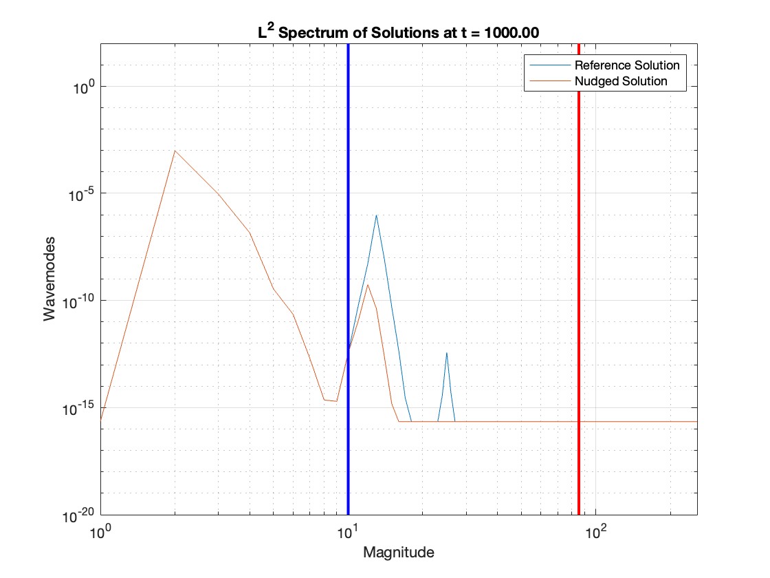
We note that in the simulations of Equation 2.6, depicted below, we utilized different spatial resolutions depending on the particular choice of initial profile and dispersion coefficient, . We ensured in our simulations that , which was consistent with the implementation of this timestepping scheme in chapter 10 of [77] and appeared to be numerically stable for all spatial resolutions we utilized in this work. Here and represent the temporal and spatial resolution scales with indicating the spatial resolution, given in powers of . While we do not explicitly state the spatial resolution for each simulation, one can see in the spectral plots, i.e. Figures 1, 2, 3, 4, 5 and 6, that the x-axis covers . In this study, ranges between and , depending on the amount of Fourier modes required to accurately simulate a given solution. is chosen specifically to ensure that the solution is well resolved, which here means that Fourier coefficients of the reference solution decay to machine precision before the dealiasing cutoff, i.e. the vertical red line featured in Figures 1, 2, 3, 4, 5 and 6. That is, the momentum decays exponentially in wave number, we take large enough such that the momentum decays to machine precision (given by ) before the wave number . We utilize 2/3 truncation for dealiasing to accurately calculate the nonlinear term, i.e., we set the last 1/3 of the Fourier modes to zero to prevent aliasing effects. Additionally, we note that while the red vertical line on spectral plots (see Figures 6(b), 6(d), 4(b) and 5(b) denotes the dealiasing cutoff, the vertical blue line denotes the observational window cutoff, that is, the Fourier modes to the left of and including the blue vertical line are accurately observed and used in the computation of the nudging term.
The nudging term is implemented numerically in Algorithm 1 as an explicit term. This implementation of the feedback-control term that we used induces a CFL constraint required for the numerical scheme to remain stable, . This CFL constraint can be removed by utilizing an implicit formulation of the nudging term, which we do not consider in this work. It is worth noting that the nudging term cannot be implemented numerically using multi-stage methods, such as RK4, due to the need to interpolate in time (see e.g. [68]). The simulations featured in this work primarily use a value of , which was found to be sufficient for this study. For an in-depth examination of the role the value of the nudging parameter plays in convergence, see [15].
To test the effectiveness of nudging on the KdV equation Equation 2.6 we utilized an “identical twin” experimental design. This experimental design is standard in the validation of data assimilation methods, where we first initialize a reference solution. This solution will be treated as the true solution which we will attempt to recover using observations. The observations will be given by the lowest Fourier modes. We note that the observations are considered to be perfect with no distortions (i.e., no error measurements) or stochastic noise.
We note that typically in the data assimilation literature for dissipative evolutionary equations, the equations are evolved forward in time long enough such that the solution remains in an absorbing set in a relevant phase space. That is, we run solutions long enough forward in time such that they are uniformly bounded with respect to time in , , or another relevant norm for all future times, see e.g., [74, 75] for a full definition of absorbing sets as well as their properties. In this study we do not evolve the equations forward in time to arbitrarily large times, as solutions are not dissipative and so there is not necessarily an absorbing set that attracts all bounded solutions after a long enough time. In fact, as the norm is a conserved quantity for Equation 2.6, such an absorbing set cannot exist in . We opted to simply evolve forward the initial profile a given amount of time, typically , in order to ensure that the reference solution has developed interesting dynamics outside the observation domain. While solutions can develop small length scales not captured by the observed modes, they typically have a finite number of active Fourier modes, with the total number of modes active at a given time dependent on the initial condition, the current time, the total momentum in the system, and the dispersion parameter, . An active Fourier mode in this sense means that , where is the wavemode index and indicates machine precision.
4. Computational Results
4.1. Classical KdV equation
In this section we will examine how the data assimilation nudging algorithm fails for Equation 2.6. Nudging appears to fail subtly, with the extent to which it works appears to be determined by whether the active Fourier modes of the initial profile are contained in the annulus of the observed Fourier modes, as we will see later on in Figure 5. We will start by considering examples such as in 2.0.5 to illustrate how nudging fails.
To find a case where nudging fails, let us consider a solution initialized on a single wavemode
| (4.1) |
where is an arbitrary constant with . Note that by 2.0.3 we know that as this solution is initially periodic, it will remain periodic for all time .
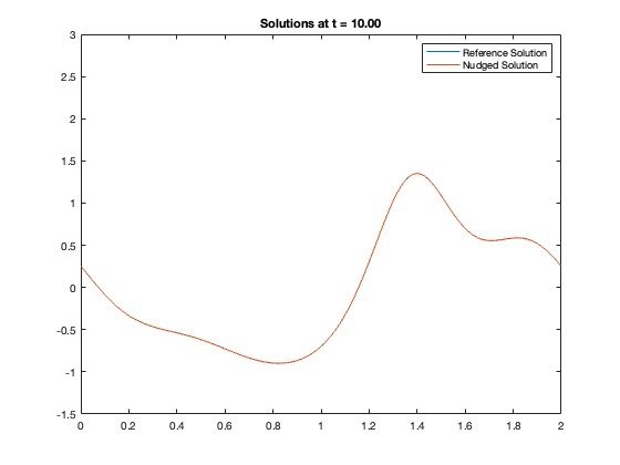
Using initial data of the form Equation 4.1 we can now construct solutions to Equation 2.6 which the nudging algorithm Equation 2.7 explicitly fails to recover. Given a number of observed modes , we can set such that . Again, we emphasize that solutions initialized in this way (see Equation 4.1) are initially periodic and remain periodic due to 2.0.3. Noting that , it follows immediately from 2.0.5 that where is the solution of Equation 2.6 generated from the initial data prescribed by Equation 4.1. This shows that a fixed number of observed Fourier modes are insufficient to distinguish the zero solution from solutions initialized with suitable high frequency oscillations, and so one should not expect data assimilation to succeed. Indeed, if we choose to be the solution of Equation 2.7 initialized by the identically zero solution, then it is easy to deduce that holds for all time and so the solution to Equation 2.7 simply corresponds to a solution to Equation 2.6 albeit with a different initial condition than the reference solution.
One can see computationally in Figure 1 that nudging fails to recover the solution , of Equation 2.6 generated from the initial data prescribed by Equation 4.1. In Figure 1 the solution, , of Equation 2.7 is initialized with the identically zero solution. Exactly as one expects, we find that holds for the entire simulation. Similarly, we see in Figure 2 the roles of and are reversed. That is, we instead initialize the solution to with Equation 4.1 and the reference solution, , is initialized with the identically zero solution. We see in Figure 2 similar behavior occurs, as the feedback-control term remains zero for the entire simulation and both equations evolve as solutions of Equation 2.6 with different initial conditions. While this is expected, it is nevertheless an interesting result as it shows that the initialization of the assimilated solution to Equation 2.7 matters. This fact is fundamentally different to many analytical results regarding the application of the nudging algorithm to dissipative equations, as for dissipative systems the effect of the initial condition fades given enough time, contrary to what occurs in this case.
The previous counterexample illustrates that data assimilation methods cannot uniquely determine the observed reference solution when the observations are identically zero, but one may hope that more physically realistic (i.e. not identically zero) observations will yield better results. This is true to some extent, however the level of success is highly dependent on the initial profile of the reference solution and one can similarly construct solutions that exhibit high frequency oscillations that nudging cannot recover. If given an analytic solution in of Equation 2.6, we can indeed construct infinitely many solutions where nudging fails to synchronize with the reference solution given a finite number of observed Fourier modes.
We will now demonstrate a general method of constructing solutions that nudging fails to synchronize. Let be a solution to Equation 2.6 such that . Here is the initial condition of . Note that the momentum is a conserved quantity of Equation 2.6, and so for all time. Now, let be given such that
| (4.2) |
By Parseval’s identity . Here is a specified constant, for computations we will use to denote machine precision. The purpose of finding such an is to separate the wavemodes into active low modes and inactive high modes. At any fixed time such an is guaranteed to exist as is analytic and therefore the Fourier coefficients must decay exponentially fast in wavenumber. In our computations we run only for a finite amount of time, so we take for to be the supremum over all such ’s taken across all simulated times. Without loss of generality we will assume that observation window consists of all modes, and so essentially the entire solution is known down to machine precision. We note here that is vital to the construction we outline below, thus examples we construct work only for finite times. This is due to the fact that we require a uniform bound on the number of active wavemodes to extend this arbitrarily far in time.
Now, we can take the given solution and use it to generate artificial solutions for which nudging appears to fail. Simply consider the solution generated by the following initial data:
| (4.3) |
Here and are positive constants chosen to enforce that and . That is, we are modifying the initial profile to take some of the momentum out of the active modes and shifting it into to wavemode , where is an arbitrary positive integer. As is arbitrary, we can construct infinitely many such solutions, all of which have the same momentum as the given solution, , but with a new active frequency in the initial profile. Note that the choice of using is arbitrary, and one can do this exact construction using the solution of evaluated at any given time.
We performed computational tests using the reference solution, , of Equation 2.6 with initial conditions prescribed by Equation 4.3. Here we took a solution, , of Equation 2.6 which was initialized simply with , which we found was suitable for the construction in Equation 4.3. Once was determined, we simply utilized , which was renormalized to ensure that . We see in Figure 3 the result from applying nudging to attempt to recover the constructed reference solution . Here the nudging solution, , of Equation 2.7 is initialized to be identically zero. We see in Figure 3 that the low modes of synchronize with to a fixed level of precision, but the reference solution contains high frequency oscillations that never develops. The error in both the high and low modes appears approximately constant after a very brief initial decay in the observed modes. We note that in additional tests (not depicted here) the same behavior in the error was observed up to time without any significant deviations in the error. One can clearly see activity in the frequencies immediately surrounding and that is simply not present in the nudged solution. Not only is this high frequency activity never generated, but nudging features no mechanism to generate targeted high mode oscillations. That is, if one knew a priori that the solution featured oscillations at wavemode , but one still only had observations of the first wavemodes, nudging does not have any mechanism to encourage oscillations at any unobserved frequencies beyond the nonlinear term.
It is worth mentioning that the construction of the initial profile in Equation 4.3 is more complex than necessary. If one were to observe the first modes of a solution with a spike at wavemode , being a positive integer, then nudging would likely fail. Here, when we say “spike”, we mean that looking at the spectrum one sees a local maximum at the specified wavemode. The construction of the initial profile in Equation 4.3 is done to produce examples where one can see by looking at the spectrum that nudging fails to develop any of the high oscillations featured in the reference solution. Indeed, we see in Figure 4 that we see similar behavior in the error to that seen in Figure 3. In Figure 4 we initialize the reference solution, , simply with , observing the first Fourier modes of . The nudging solution, , of Equation 2.7, was initialized to be identically zero. We see in Figure 4 that the nudged solution still fails to develop all the high frequencies present in the reference solution, even at time .
We note that the simulations presented here indicate that nudging is ill-suited to extremely capture high oscillatory solutions to Equation 2.6, but it does not necessarily prohibit other methods of data assimilation from recovering the reference solution. Unlike in Figure 2, where the observed data is identically zero, it is not impossible in theory for data assimilation to tell the difference between two solutions initialized of the form Equation 4.1. That is, unlike the case of Figure 2 if one initializes two solutions and of Equation 2.6 with initial data prescribed by Equation 4.1 with separate values for and , we have that for , and to the best of our knowledge one cannot readily construct two such solutions of this form that always agree on every observed wavemode for all time. This is due to the fact that dispersive term essentially causes the coefficients of the wavemodes to rotate in the complex plane around the origin with rotation speed . As each wavemode is rotating at a different speed one cannot rescale and shift momentum across wavemodes in a straightforward way such that the momentum backscattering due to the nonlinearity on the observed modes still agree at each timestep to produce a counterexample similar to the one present in Figures 2 and 1.
We note that all of these cases where nudging fails are specific to the undamped and unforced, classical KdV Equation 2.6, which is not a dissipative dynamical system. The addition of damping will result in the energy being drained from these high oscillations, while the forcing injects energy into specified low wavemodes, resulting in nontrivial long time dynamics that eliminate these sorts of extremely high frequency oscillations, see Section 4.2 below.


4.2. Damped and Driven KdV
In this subsection we examine the case of the damped and driven KdV equation, that is, we study the following equation:
| (4.4) |
subject to periodic boundary conditions. Here is the damping coefficient constant and is a body force that is given to be constant in time with zero spatial average. The corresponding nudged damped and driven KdV equation is given by
| (4.5) |
In [55] it was shown analytically, that given enough observed Fourier modes and large enough , that the nudged solution converges to the reference solution in exponentially fast in time with exponent for arbitrary choice of initial data with spatial mean zero for Equation 4.5.
We now verify computationally that nudging successfully drives the assimilated solution to the reference solution exponentially fast in time. Depicted in Figure 6 we can see nudging effectively recovers a reference solutions initialized as in Equation 4.1 exponentially fast in time. Here we utilize and and we note that the exponential rate of convergence is given by small perturbations from . Here we initialize the reference solution as in Equation 4.1 with , that is, we selected the initial profile . For our driving force, we utilized . We note that and we observed only the first 10 modes of the solution. It is unsurprising that convergence happens at the exponential rate proportional to the damping coefficient, , as this coincides with the results of [55]. We note that the exponential convergence is not entirely independent of , the oscillatory component at initial times and on the observed modes is particularly sensitive to values, although this effect quickly fades as the error begins to decay at rate . Moreover, as one sees from the spectrum plots in Figure 6 the primary barrier for convergence are the spikes in undetected frequencies, therefore it is unsurprising that convergence to the reference solution happens at exactly the rate, , at which momentum is drained from these modes. Indeed, this behavior is typical of simulations of nudging methods, as the unobserved modes rely on the dissipation in the system in order to synchronize. The overall decay in error can typically be decomposed into two distinct phases, an initial rapid decay in error that is highly dependent on , and a slower, but still exponentially fast in time, rate of convergence primarily driven by the dissipation in the system. For an in-depth study of the role of the particular value of see, e.g., [15].
We note that the AOT algorithm successfully recovers the reference solution, , to Equation 4.4 even when is initialized as in the counterexamples from the previous section Equations 4.1 and 4.3 given enough observed modes. We also point out, that in Figure 6 we see some behavior in the observed modes due to the presence of the body force. We could disable the body force by setting it to , however in that case data assimilation would not be required at all. This is because the damping term will drive any initial condition to , exponentially fast at the rate with or without any form of data assimilation being applied.


5. Lorenz 1963 System
As the focus of this work is examining the applicability of the AOT algorithm to dynamical systems that are not dissipative, we now turn to examine a nondissipative variant of the Lorenz 1963 system. Lorenz introduced in 1963 a simplified/reduced model of atmospheric convection [64], and so it is of particular interest for studying methods of data assimilation, see e.g. [49, 12, 29, 48, 70, 63] and the references within. The 1963 Lorenz system is given by:
| (5.1) |
Here is the Prandtl number, is the Rayleigh number, and is a geometric factor. It is well-known that, for certain parameter choices (e.g., , , ), that the Lorenz system has a chaotic global attractor [78].
It is also known that applying the AOT algorithm, or a synchronization scheme, as in [49, 48], by observing only the component is sufficient to synchronize the nudged solution with the reference solution (see e.g. [49, 12, 48]). In particular, we can consider the following three synchronization schemes from [48] (which was motivated by [68]) to understand when data assimilation works for this system.
| (5.2) |
| (5.3) |
| (5.4) |
The above equations, Equations 5.2, 5.3 and 5.4, correspond to the regimes when the observed values of , , or , respectively, are observed and inserted directly into the equations for the remaining, unobserved components. That is, e.g. in Equation 5.2 we observe the true value of continuously in time and insert that into the evolution equations of and . In these equations we note that numerically we should not be simulating the evolution of , , or as they appear in Equations 5.2, 5.3 and 5.4, respectively, but rather these values are observed (given) from the true solution in Equation 5.1 and are inserted directly into the equations for the remaining variables. Analysis on Equations 5.2, 5.3 and 5.4 was conducted in [48] where it was shown that the continuous coupling on or alone was sufficient to obtain synchronization between the assimilated equations and the reference solution, however the coupling seen in Equation 5.4 was not sufficient to obtain convergence in either the or components to the corresponding components or of the true solution. We do note that in [48] the equations for Equation 5.1 were written in a slightly different form, however this can be easily reconciled by using the transformation .
For the sake of completeness, we will discuss the convergence results for the above systems, Equations 5.2, 5.3 and 5.4 proven in [48] and discuss how the results break down in the absence of dissipation. Let
| (5.5) |
where is the given solution of Equation 5.1 and is the solution to one of the assimilated equation, Equations 5.2, 5.3 and 5.4. Here we define with the understanding that the variable in missing from the assimilated equation is taken to be equal to the corresponding variable in Equation 5.1, e.g. when considering Equation 5.2 we define for all time, and have . The convergence results for the synchronization algorithms, Equations 5.2, 5.3 and 5.4 are given as follows:
Theorem 5.0.1 (Hayden (2007) [48]).
Let , be the solution to Equation 5.1, then the following are true when and .
If is the solution to Equation 5.2, then
| (5.6) |
The proofs of 5.0.1 are derived by taking the difference of the assimilated equation (Equation 5.2 or Equation 5.3) with Equation 5.1, summing the squares of the derivatives, and applying Grönwall’s inequality to the resulting quantity. The estimate in Equation 5.7 arises from the use of the global bound
| (5.9) |
which was derived in [28] and was used to bound the contribution from the nonlinear term in the equation.
We note that the analysis done in the proof of 5.0.1 is dependent on the particular parameters and requires , and . To illustrate how these sorts of estimates break down in the absence of dissipation, we consider the case when both and are observed, i.e., are given from the true solution of Equation 5.1. This leads to the following system of equations
| (5.10) |
Now, if we take , where solves Equation 5.1, we see from Equations 5.1 and 5.10 that satisfies the following equation
| (5.11) |
From here, we can see that if , we can multiply both sides by and apply Grönwall’s inequality to obtain
| (5.12) |
which yields convergence of to exponentially fast in time. If we instead consider , removing the dissipation on the component of Equation 5.1, then we now have that , and so holds for all time. Therefore, we have that the absence of dissipation on the component prevents synchronization between the assimilated solution and the reference solution, even when both the and components are observed continuously in time.
We note that the above discussion has been on the synchronization data assimilation scheme, given by the direct insertion, as it was first introduced in [68], of the observed quantities into the model equations. We now consider the nudged Lorenz system for the observed and components of Equation 5.1, given as follows:
| (5.13) |
Here is the nudging coefficient, which controls the strength of the feedback-control terms. For simplicity, we utilize the same nudging parameter, , in the equations for and , however this is not strictly necessary.
At any fixed time, , the solutions, , to the nudged equations, Equation 5.13, are expected to converge to the solution of the synchronization algorithm, given by Equation 5.10 as . This can be justified rigorously by applying the argument present in [15] to the Lorenz 1963 system, provided both methods are initialized with the same initial data. An analogous statement was made in [72] for the Lorenz system in particular (with ), where it was shown that the solution, , of Equation 5.13, converges to at any fixed time, , as we send when the nudging term is present only on the equation for in Equation 5.13. In the case where , if we assume a priori that the solutions of Equation 5.13 converge to those of Equation 5.10 as , one can deduce using the reverse triangle inequality, that , where is given as defined previously in Equation 5.5. Therefore, we expect the nudged Lorenz system, Equation 5.13, to fail to recover the true solution in the same way that Equation 5.10 fails when dissipation is removed from the equations for .
We now demonstrate numerically that this dissipation mechanism (when ) of the Lorenz system is necessary for data assimilation methods to work. In particular, we will be considering a partially dissipative variant of the Lorenz system by taking , i.e., eliminating the dissipation mechanism only on the component. The analytical results regarding the nudging algorithm applied to the Lorenz equations have been done when and are qualitatively similar to those we reference above in 5.0.1 from [48], see e.g. [12, 72, 17]. That is, the solutions of Equation 5.13 synchronize with those of Equation 5.1 exponentially fast in time for large enough nudging parameter values and with the exponential rate depending on the particular parameters of Equation 5.1. While nudging is only required on either the or components in order to drive convergence, we will utilize nudging on both the and components to emphasize that, even with additional nudging, the method is not effective when the dissipation on the -component is eliminated (i.e. when ).
We have numerically implemented the Lorenz system as in [12, 72] using an explicit Euler scheme for the time discretization. As in [72], we will utilize for our timestep. We note that in many works the reference solution is initialized by running the solution forward in time until it is approximately on the global attractor (see e.g. [12, 49]), however as we are attempting to test nudging for non-dissipative or partially dissipative systems, which need not possess global attractors, we will instead be utilizing the initial data as in [72].
First, we verify the validity of nudging on the Lorenz system with full dissipation. Using the initial data and parameter choices discussed previously we apply nudging to the Lorenz system with . The results can be seen in Figure 7, where we have applied nudging to only the first two components of Equation 5.13. Here we can see that all variables converge to an error level of approximately with spurious dips below this error level in each component. Note that here we see exponential convergence to the true solution, as we expect in this case.

Next, we examine what happens when we apply nudging for the partially dissipative Lorenz system, i.e., with . The results can be seen in Figure 8. Note that here we still see exponential decay to the true solution in both and . While nudging appears to affect initially, this effect quickly fades after a short interval of time and the error appears to stabilize to be approximately constant . The error level that is attained appears to be directly linked to the difference in the initial conditions for the component. To illustrate this, we plotted the (Euclidean norm) error over time when both the reference and nudged equations are initialized with the same initial data, except for the component. Here and , where ranges in values from to . The results of these tests can be seen in Figure 9 and they illustrate that the error is highly sensitive to small perturbations in the initial condition for . We note that the behavior seen in Figure 9 appears to align with what one should expect from our earlier discussion of Equation 5.11 for the synchronization algorithm. We note that we obtain an initial exponential decay in the error in the component which is driven by the convergence in both and . This initial convergence levels off and becomes approximately constant as and converge to and , respectively.


6. Conclusion
Based on the results of the simulation presented in Section 4, we conclude that the AOT data assimilation algorithm is unsuitable for non-dissipative or partially dissipative dynamical systems, such as the KdV equation, Equation 2.6, and the partially dissipative Lorenz system, Equation 5.1. In fact, we conclude that the pathologic counterexamples used in Section 4.1 present an insurmountable challenge for any method of data assimilation to recover. In particular, we note that counterexample we utilize in Figure 1 will fail for any method of data assimilation, as the true solution has no discernible impact on the observed modes, and so it is impossible to reliably tell the true solution apart from the zero solution (or one of an infinite number of solutions one can readily construct) based solely on the observations. Moreover, the counter examples considered in Section 4.1 are not specific to the KdV equation. The particular solutions considered in 2.0.5 were constructed due to the periodic invariance induced by the convolutional Fourier mode structure of the nonlinear term (see 2.0.4), and thus one can construct similar counter examples for other non-dissipative systems with this same nonlinearity, such as the inviscid Burgers equations.
In addition to showing that data assimilation simply doesn’t work for certain pathological counterexamples, we note that the extent to which data assimilation does work for the classical KdV equation may be highly dependent on the choice of initial data for the nudged system, . Indeed, while it was proved in [4] that for 2D NSE the choice of initial data was arbitrary, we have here that data assimilation will simply fail if not initialized properly, as it does in Figure 1. The problem of initialization is one of the core strengths of the nudging algorithm, and so it is worth noting that this property fails to hold for a system without finitely many determining modes.
We note that data assimilation could be made to work if one were to assume more of the true solution. For instance, if one were to assume that the solution was supported on an annulus in Fourier space, one could eliminate all the examples that we study here. We caution anyone against doing this, however, as imposing these sorts of restrictions on the solution can trivialize the dynamics of equations in a way that may not be physical.
Acknowledgments
This research was supported in part by NPRP grant # S-0207-359200290 from the Qatar National Research Fund (a member of Qatar Foundation). The work of E.S.T. was also supported by King Abdullah University of Science and Technology (KAUST) Office of Sponsored Research (OSR) under Award No. OSR-2020-CRG9-4336.
References
- [1] Débora A.F. Albanez, Helena J. Nussenzveig Lopes, and Edriss S. Titi. Continuous data assimilation for the three-dimensional Navier–Stokes- model. Asymptotic Anal., 97(1-2):139–164, 2016.
- [2] M. U. Altaf, E. S. Titi, O. M. Knio, L. Zhao, M. F. McCabe, and I. Hoteit. Downscaling the 2D Benard convection equations using continuous data assimilation. Comput. Geosci, 21(3):393–410, 2017.
- [3] Richard A. Anthes. Data assimilation and initialization of hurricane prediction models. J. Atmos. Sci., 31(3):702–719, 1974.
- [4] Abderrahim Azouani, Eric Olson, and Edriss S. Titi. Continuous data assimilation using general interpolant observables. J. Nonlinear Sci., 24(2):277–304, 2014.
- [5] Abderrahim Azouani and Edriss S. Titi. Feedback control of nonlinear dissipative systems by finite determining parameters—a reaction-diffusion paradigm. Evol. Equ. Control Theory, 3(4):579–594, 2014.
- [6] Hakima Bessaih and Franco Flandoli. Weak attractor for a dissipative Euler equation. Journal of Dynamical and Differential Equations, 12:713–732, 2000.
- [7] Hakima Bessaih, Eric Olson, and Edriss S. Titi. Continuous data assimilation with stochastically noisy data. Nonlinearity, 28(3):729–753, 2015.
- [8] Animikh Biswas, Zachary Bradshaw, and Michael S. Jolly. Data assimilation for the Navier-Stokes equations using local observables. SIAM J. Appl. Dyn. Syst., 20(4):2174–2203, 2021.
- [9] Animikh Biswas, Ciprian Foias, Cecilia F. Mondaini, and Edriss S. Titi. Downscaling data assimilation algorithm with applications to statistical solutions of the Navier–Stokes equations. In Annales de l’Institut Henri Poincaré C, Analyse non linéaire, pages 295–326. Elsevier, 2019.
- [10] Animikh Biswas and Vincent R. Martinez. Higher-order synchronization for a data assimilation algorithm for the 2D Navier–Stokes equations. Nonlinear Anal. Real World Appl., 35:132–157, 2017.
- [11] Animikh Biswas and Randy Price. Continuous data assimilation for the three dimensional Navier-Stokes equations. (submitted) arXiv 2003.01329.
- [12] Jordan Blocher, Vincent R Martinez, and Eric Olson. Data assimilation using noisy time-averaged measurements. Physica D: Nonlinear Phenomena, 376:49–59, 2018.
- [13] Jerry L. Bona and Ronald Smith. The initial-value problem for the Korteweg-de Vries equation. Philosophical Transactions of the Royal Society of London. Series A, Mathematical and Physical Sciences, 278(1287):555–601, 1975.
- [14] W. P. Budgell. Nonlinear data assimilation for shallow water equations in branched channels. Journal of Geophysical Research: Oceans, 91(C9):10633–10644, 1986.
- [15] Elizabeth Carlson, Aseel Farhat, Vincent Martinez, and Collin Victor. On the infinite-nudging limit of the nudging filter for continuous data assimilation. arXiv preprint arXiv:2408.02646, 2024.
- [16] Elizabeth Carlson, Joshua Hudson, and Adam Larios. Parameter recovery for the 2 dimensional Navier-Stokes equations via continuous data assimilation. SIAM J. Sci. Comput., 42(1):A250–A270, 2020.
- [17] Elizabeth Carlson, Joshua Hudson, Adam Larios, Vincent R Martinez, Eunice Ng, and Jared P Whitehead. Dynamically learning the parameters of a chaotic system using partial observations. Discrete and Continuous Dynamical Systems, 42(8):3809–3839, 2022.
- [18] Elizabeth Carlson and Adam Larios. Sensitivity analysis for the 2D Navier–Stokes equations with applications to continuous data assimilation. Journal of Nonlinear Science, 31(5):84, 2021.
- [19] Elizabeth Carlson, Ṽan Roekel, Luke, Mark Petersen, Humberto C. Godinez, and Adam Larios. CDA algorithm implemented in MPAS-O to improve eddy effects in a mesoscale simulation. 2021. (submitted).
- [20] Emine Celik and Eric Olson. Data assimilation using time-delay nudging in the presence of Gaussian noise. Journal of Nonlinear Science, 33(6):110, 2023.
- [21] Nan Chen, Yuchen Li, and Evelyn Lunasin. An efficient continuous data assimilation algorithm for the Sabra shell model of turbulence, 2021.
- [22] Vladimir V. Chepyzhov and Mark I. Vishik. Trajectory attractors for dissipative 2D Euler and Navier–Stokes equations. Russian Journal of Mathematical Physics, 15:156–170, 2008.
- [23] Vladimir V. Chepyzhov, Mark I. Vishik, and Sergey V. Zelik. Strong trajectory attractors for dissipative Euler equations. Journal de Mathématiques Pures et Appliquées, 96(4):395–407, 2011.
- [24] Patricio Clark Di Leoni, Andrea Mazzino, and Luca Biferale. Inferring flow parameters and turbulent configuration with physics-informed data assimilation and spectral nudging. Physical Review Fluids, 3(10):104604, 2018.
- [25] B. Cockburn, D.A. Jones, and E.S. Titi. Estimating the number of asymptotic degrees of freedom for nonlinear dissipative systems. Math. Comput., 66:1073–1087, 1997.
- [26] S. Desamsetti, H.P. Dasari, S. Langodan, O. Knio, I. Hoteit, and Edriss S. Titi. Efficient dynamical downscaling of general circulation models using continuous data assimilation. Quarterly Journal of the Royal Meteorological Society, 2019.
- [27] Amanda E. Diegel and Leo G. Rebholz. Continuous data assimilation and long-time accuracy in a interior penalty method for the Cahn-Hilliard equation. Appl. Math. Comput., 424:Paper No. 127042, 22, 2022.
- [28] Charles R. Doering and J. D. Gibbon. Applied Analysis of the Navier–Stokes Equations. Cambridge Texts in Applied Mathematics. Cambridge University Press, Cambridge, 1995.
- [29] Yi Juan Du and Ming-Cheng Shiue. Analysis and computation of continuous data assimilation algorithms for Lorenz 63 system based on nonlinear nudging techniques. Journal of Computational and Applied Mathematics, 386:113246, 2021.
- [30] Tarek Elgindi, Wenqing Hu, and Vladimír Šverák. On 2d incompressible Euler equations with partial damping. Communications In Mathematical Physics, 355(1):145–159, 2017.
- [31] Aseel Farhat, Michael S. Jolly, and Edriss S. Titi. Continuous data assimilation for the 2D Bénard convection through velocity measurements alone. Phys. D, 303:59–66, 2015.
- [32] Aseel Farhat, Evelyn Lunasin, and Edriss S. Titi. Abridged continuous data assimilation for the 2D Navier–Stokes equations utilizing measurements of only one component of the velocity field. J. Math. Fluid Mech., 18(1):1–23, 2016.
- [33] Aseel Farhat, Evelyn Lunasin, and Edriss S. Titi. Data assimilation algorithm for 3D Bénard convection in porous media employing only temperature measurements. J. Math. Anal. Appl., 438(1):492–506, 2016.
- [34] Aseel Farhat, Evelyn Lunasin, and Edriss S. Titi. On the Charney conjecture of data assimilation employing temperature measurements alone: the paradigm of 3D planetary geostrophic model. Mathematics of Climate and Weather Forecasting, 2(1), 2016.
- [35] Aseel Farhat, Evelyn Lunasin, and Edriss S. Titi. Continuous data assimilation for a 2D Bénard convection system through horizontal velocity measurements alone. J. Nonlinear Sci., pages 1–23, 2017.
- [36] C. Foias, O. Manley, R. Rosa, and R. Temam. Navier–Stokes Equations and Turbulence, volume 83 of Encyclopedia of Mathematics and its Applications. Cambridge University Press, Cambridge, 2001.
- [37] C. Foiaş and G. Prodi. Sur le comportement global des solutions non-stationnaires des équations de Navier-Stokes en dimension . Rend. Sem. Mat. Univ. Padova, 39:1–34, 1967.
- [38] Ciprian Foias, Cecilia F. Mondaini, and Edriss S. Titi. A discrete data assimilation scheme for the solutions of the two-dimensional Navier–Stokes equations and their statistics. SIAM J. Appl. Dyn. Syst., 15(4):2109–2142, 2016.
- [39] K. Foyash, M. S. Dzholli, R. Kravchenko, and È. S. Titi. A unified approach to the construction of defining forms for a two-dimensional system of Navier–Stokes equations: the case of general interpolating operators. Uspekhi Mat. Nauk, 69(2(416)):177–200, 2014.
- [40] Trenton Franz, Adam Larios, and Collin Victor. The bleeps, the sweeps, and the creeps: Convergence rates for observer patterns via data assimilation for the 2d Navier-Stokes equations. Comput. Methods Appl. Mech. Engrg., 392:Paper No. 114673, 19, 2022.
- [41] Bosco García-Archilla and Julia Novo. Error analysis of fully discrete mixed finite element data assimilation schemes for the Navier-Stokes equations. Adv. Comput. Math., 46(4):Paper No. 61, 33, 2020.
- [42] Bosco García-Archilla, Julia Novo, and Edriss S. Titi. Uniform in time error estimates for a finite element method applied to a downscaling data assimilation algorithm for the Navier-Stokes equations. SIAM J. Numer. Anal., 58(1):410–429, 2020.
- [43] M. Gardner, A. Larios, L. G. Rebholz, D. Vargun, and C. Zerfas. Continuous data assimilation applied to a velocity-vorticity formulation of the 2d Navier-Stokes equations. Electronic Research Archive, 29(3):2223–2247, 2021.
- [44] Masakazu Gesho, Eric Olson, and Edriss S. Titi. A computational study of a data assimilation algorithm for the two-dimensional Navier–Stokes equations. Commun. Comput. Phys., 19(4):1094–1110, 2016.
- [45] J-M. Ghidaglia. Weakly damped forced Korteweg-de Vries equations behave as a finite dimensional dynamical system in the long time. Journal of Differential Equations, 74:369–390, 1988.
- [46] J-M. Ghidaglia. A note on the strong convergence towards attractors of damped forced KdV equations. Journal of Differential Equations, 110:356–359, 1994.
- [47] Shandy Hauk. The long-time behavior of the Stommel-Charney model of the gulf-stream: An analytical and computational study. PhD thesis, Department of Mathematics, University of California - Irvine, 1997.
- [48] Kevin Hayden. Synchronization in the Lorenz System. PhD thesis, Masters Thesis, University of Nevada, Department of Mathematics and Statistics, 2007.
- [49] Kevin Hayden, Eric Olson, and Edriss S. Titi. Discrete data assimilation in the Lorenz and 2D Navier–Stokes equations. Phys. D, 240(18):1416–1425, 2011.
- [50] James E Hoke and Richard A Anthes. The initialization of numerical models by a dynamic-initialization technique. Monthly Weather Review, 104(12):1551–1556, 1976.
- [51] Hussain A Ibdah, Cecilia F Mondaini, and Edriss S. Titi. Fully discrete numerical schemes of a data assimilation algorithm: uniform-in-time error estimates. IMA Journal of Numerical Analysis, 40(4):2584–2625, 2020.
- [52] Alexei A. Ilyin and Edriss S. Titi. On the domain of analyticity and small scales for the solutions of the damped-driven 2D Navier–Stokes equations. Dyn. Partial Differ. Equ., 4(2):111–127, 2007.
- [53] Michael S. Jolly, Vincent R. Martinez, Eric J. Olson, and Edriss S. Titi. Continuous data assimilation with blurred-in-time measurements of the surface quasi-geostrophic equation. Chin. Ann. Math. Ser. B, 40(5):721–764, 2019.
- [54] Michael S. Jolly, Vincent R. Martinez, and Edriss S. Titi. A data assimilation algorithm for the subcritical surface quasi-geostrophic equation. Adv. Nonlinear Stud., 17(1):167–192, 2017.
- [55] Michael S. Jolly, Tural Sadigov, and Edriss S. Titi. Determining form and data assimilation algorithm for weakly damped and driven Korteweg–de Vries equation—Fourier modes case. Nonlinear Analysis: Real World Applications, 36:287–317, 2017.
- [56] Don A. Jones and Edriss S. Titi. Determining finite volume elements for the 2D Navier–Stokes equations. Phys. D, 60(1-4):165–174, 1992. Experimental mathematics: computational issues in nonlinear science (Los Alamos, NM, 1991).
- [57] Aly-Khan Kassam and Lloyd N. Trefethen. Fourth-order time-stepping for stiff PDEs. SIAM J. Sci. Comput., 26(4):1214–1233, 2005.
- [58] N.KR. Kevlahan, R. Khan, and B. Protas. On the convergence of data assimilation for the one-dimensional shallow water equations with sparse observations. Advances in Computational Mathematics, 45:3195–3216, 2019.
- [59] Adam Larios and Yuan Pei. Nonlinear continuous data assimilation. arXiv:1703.03546.
- [60] Adam Larios and Yuan Pei. Approximate continuous data assimilation of the 2D Navier–Stokes equations via the Voigt-regularization with observable data. Evol. Equ. Control Theory, 9(3):733–751, 2020.
- [61] Adam Larios, Leo G. Rebholz, and Camille Zerfas. Global in time stability and accuracy of IMEX-FEM data assimilation schemes for Navier-Stokes equations. Computer Methods in Applied Mechanics and Engineering, 2018.
- [62] Adam Larios and Collin Victor. Continuous data assimilation with a moving cluster of data points for a reaction diffusion equation: A computational study. Commun. Comp. Phys., 29:1273–1298, 2021.
- [63] Kody Law, Abhishek Shukla, and Andrew Stuart. Analysis of the 3DVAR filter for the partially observed Lorenz ’63 model, 2014.
- [64] Edward N Lorenz. Deterministic nonperiodic flow. Journal of atmospheric sciences, 20(2):130–141, 1963.
- [65] Evelyn Lunasin and Edriss S. Titi. Finite determining parameters feedback control for distributed nonlinear dissipative systems—a computational study. Evol. Equ. Control Theory, 6(4):535–557, 2017.
- [66] Peter A. Markowich, Edriss S. Titi, and Saber Trabelsi. Continuous data assimilation for the three-dimensional Brinkman-Forchheimer-extended Darcy model. Nonlinearity, 29(4):1292–1328, 2016.
- [67] Cecilia F. Mondaini and Edriss S. Titi. Uniform-in-time error estimates for the postprocessing Galerkin method applied to a data assimilation algorithm. SIAM J. Numer. Anal., 56(1):78–110, 2018.
- [68] Eric Olson and Edriss S. Titi. Determining modes and grashof number in 2D turbulence: a numerical case study. Theor. Comp. Fluid Dyn., 22(5):327–339, 2008.
- [69] Benjamin Pachev, Jared P. Whitehead, and Shane A. McQuarrie. Concurrent multi-parameter learning demonstrated on the Kuramoto-Sivashinsky equation. SIAM J. Sci. Comput., 44(5):A2974–A2990, 2022.
- [70] Louis M Pecora and Thomas L Carroll. Synchronization in chaotic systems. Physical review letters, 64(8):821, 1990.
- [71] Yuan Pei. Continuous data assimilation for the 3D primitive equations of the ocean. Comm. Pure Appl. Math., 18(2):643, 2019.
- [72] Yu Chen Peng, Liang Chun Wu, and Ming-Cheng Shiue. Finite time synchronization of the continuous/discrete data assimilation algorithms for Lorenz 63 system based on the back and forth nudging techniques. Results in Applied Mathematics, 20:100407, 2023.
- [73] Leo G. Rebholz and Camille Zerfas. Simple and efficient continuous data assimilation of evolution equations via algebraic nudging. Numer Methods Partial Differential Eq., pages 1–25, 2021.
- [74] J. C. Robinson. Infinite-Dimensional Dynamical Systems. Cambridge Texts in Applied Mathematics. Cambridge University Press, Cambridge, 2001. An Introduction to Dissipative Parabolic PDEs and the Theory of Global Attractors.
- [75] R. Temam. Infinite-Dimensional Dynamical Systems In Mechanics and Physics, volume 68 of Applied Mathematical Sciences. Springer-Verlag, New York, second edition, 1997.
- [76] Seshu Tirupathi, Tigran T. Tchrakian, Sergiy Zhuk, and Sean McKenna. Shock capturing data assimilation algorithm for 1d shallow water equations. Advances in Water Resources, 88:198–210, 2016.
- [77] Lloyd N. Trefethen. Spectral Methods in MATLAB, volume 10 of Software, Environments, and Tools. Society for Industrial and Applied Mathematics (SIAM), Philadelphia, PA, 2000.
- [78] Warwick Tucker. The Lorenz attractor exists. Comptes Rendus de l’Académie des Sciences - Series I - Mathematics, 328(12):1197–1202, 1999.
- [79] N. J. Zabusky and M. D. Kruskal. Interaction of ”solitons” in a collisionless plasma and the recurrence of initial states. Phys. Rev. Lett., 15:240–243, Aug 1965.
- [80] Camille Zerfas, Leo G. Rebholz, Michael Schneier, and Traian Iliescu. Continuous data assimilation reduced order models of fluid flow. Comput. Methods Appl. Mech. Engrg., 357:112596, 18, 2019.