On the Feasible Region of Efficient Algorithms for Attributed Graph Alignment

The graph alignment problem, also referred to as the graph matching or noisy graph isomorphism problem, is the problem of finding the correspondence between the vertices of two correlated graphs. This problem has been given increasing attention for its applications in social network de-anonymization. For instance, datasets of social networks are typically anonymized for privacy protection. However, an attacker may be able to de-anonymize the dataset by aligning its user-user connection graph with that of publicly available data. Attributed graph alignment is a variant of graph alignment in which side information, referred to as attributes of vertices, is also publicly available in addition to the user-user connection information. This variant is motivated by the fact that there might exist publicly available attribute information in social networks. For example, the anonymized network Netflix has users’ movie-watching history and ratings publicly available. Moreover, the examination of the proposed model provides both achievability and converse results for various well-known variations of the Erdős–Rényi graph alignment problems. These variations include the traditional graph alignment problem without attributes, the seeded graph alignment problem, and the bipartite alignment problem. Consequently, the study of attributed graph alignment introduces a novel perspective for investigating these problems within an integrated framework.

In this paper, we focus on the attributed graph alignment problem under the attributed Erdős–Rényi pair model $\mathcal{G}(n,p,s_{\mathrm{u}};m,q,s_{\mathrm{a}})$, first proposed in [1]. In this model, a base graph $G$ is generated on the vertex set $[n+m]$ where the vertices from the set $[n]$ represent users and the rest of the vertices represent attributes. Between each pair of users, an edge is generated independently and identically with probability $p$ to represent their connection. For each user-attribute pair, an edge is generated independently and identically with probability $q$ to represent their association. Note that there are no edges between attributes. The graph $G$ is then independently subsampled to two graphs $G_{1}$ and $G_{2}$, where each user-user edge is subsampled with probability $s_{\mathrm{u}}$ and each user-attribute edge is subsampled with probability $s_{\mathrm{a}}$. To model the anonymization procedure, a random permutation $\Pi^{*}$ chosen uniformly at random is applied to the users in $G_{2}$ to generate an anonymized version $G_{2}^{\prime}$. Our goal in this model is to achieve exact alignment, i.e., to exactly recover the permutation $\Pi^{*}$ using $G_{1}$ and $G_{2}^{\prime}$.

For the attributed graph alignment problem, and the graph alignment problem in general, two often asked questions are the following. First, for what region of graph statistics is exact alignment feasible with unlimited computational power? This region is usually referred to as the information-theoretically feasible region or the information-theoretic limits. Second, for what region of graph statistics is exact alignment feasible with polynomial-time algorithms? This region is usually referred to as the feasible region of polynomial-time algorithms. Characterizing these two feasible regions and their relationship is of utmost importance to developing a fundamental understanding of the graph alignment problem.

There has been extensive studies on these two questions under the Erdős–Rényi pair model without attributes. A line of research focuses on the information-theoretic limits of exact alignment [2, 3, 4, 5]. Roughly speaking, it is shown that exact alignment is information-theoretically feasible when the intersection graph is dense enough. A sharp threshold of exact alignment has been established, while there still exists some gap between the converse and the achievability results. Another line of research focuses on polynomial-time algorithms for exact alignment [6, 7, 8, 9, 10]. Compared to the information-theoretic limits, the existing polynomial-time algorithms further require higher edge correlation between the pair of graphs to achieve exact alignment. The question of whether there exists polynomial-time algorithms that achieve the known information-theoretic limits is still left open.

For the attributed graph alignment problem, the information-theoretic limit has been studied in [1], where the feasible region (achievability results) and infeasible region (converse results) are characterized with a gap in between in some regimes. However, the feasible region of polynomial-time algorithms for attributed graph alignment has not been studied before, and it is the focus of this paper. In this work, we propose two polynomial-time algorithms for attributed graph alignment and characterize their feasible regions. The two algorithms are designed for two different regimes of parameters based on the richness of attribute information: the algorithm AttrRich is designed for the regime where $mqs_{\mathrm{a}}^{2}=\Omega(\log n)$, referred to as the attribute-information rich regime; and the algorithm AttrSparse is designed for the regime where $mqs_{\mathrm{a}}^{2}=o(\log n)$, referred to as the attribute-information sparse regime. In both algorithms, we first explore the user-attribute connections to align a set of anchor users, and then utilize the user-user connections to the anchors to align the rest of users. Due to the regime difference, AttrRich is able to generate a much larger set of anchors in the first step than AttrSparse. Therefore, AttrRich and AttrSparse make use of the anchors differently in the second step: AttrRich explores one-hop user-user connections to align the rest of users, while AttrSparse explores one-hop or multiple-hop user-user connections to align the rest of users depending on the sparsity of user-user connections. This idea of matching vertices based on common neighbor witnesses has been explored to construct efficient graph alignment algorithms under the context of seeded graph alignment [11, 12, 13, 14]. In this work, we employ this idea in a two-step procedure under the setting of attributed graphs, and analyze its performance through a careful treatment of the dependency between the two steps.

Our characterizations of the feasible regions of AttrRich and AttrSparse are illustrated in Figure 1 as areas and , respectively. The information-theoretically feasible and infeasible regions given in [1] are also illustrated in the figure for comparison. We can see that there is a gap between the feasible region achieved by AttrRich and AttrSparse and the known information-theoretically feasible region. It is left open whether this gap is a fundamental limit of polynomial-time algorithms ¹¹1We comment that in the line of work [15, 16, 17], the authors have explored efficient algorithms for a closely-related problem known as attributed network alignment. In this problem, attributes are attached to both vertices and edges, in contrast to the exclusive association with vertices in attributed graph alignment. The focus in this line of work is the empirical performance rather than the theoretical feasible region.

In addition, we specialize the feasible region of the proposed algorithms to the context of the seeded Erdős–Rényi graph alignment problem, and demonstrate that the specialized feasible region includes certain range of parameters that is not known to be achievable in the literature.

Our results reveal that attributes possibly facilitate graph alignment in a much more significant way when computational efficiency is a priority. We demonstrate this possible impact of attributes under the sparse regime $np=\Theta(\log n)$ in Figure 2. In Figure 2(a), we let $mqs_{\mathrm{a}}^{2}=0$ so there is no information from the attributes, which is equivalent to the graph alignment problem without attributes; in Figure 2(b), we let $mqs_{\mathrm{a}}^{2}=0.1\log n$. We keep $p=o(1)$, and assume the value of $nps_{\mathrm{u}}/\log n$ can be an arbitrarily large constant but not tending to infinity in both settings for ease of comparison. Comparing these two figures, we can see that when $mqs_{\mathrm{a}}^{2}$ increases from $0$ to $0.1\log n$, the information-theoretic limits in terms of user-user parameters ($n,p$ and $s_{\mathrm{u}}$) improve a bit as expected. However, a more fundamental improvement is in the feasible region achievable by polynomial-time algorithms. In Figure 2(a), the green region above $s_{\mathrm{u}}=\sqrt{\alpha}$ is achievable by a polynomial-time algorithm proposed in [10], where $\alpha\approx 0.338$ is known as the Otter’s constant. The red region below $s_{\mathrm{u}}=\sqrt{\alpha}$ is not known to be achievable by any polynomial-time algorithms. Moreover, in [18], this red region is conjectured to be infeasible by any polynomial-time algorithm.²²2We note that the conjecture presented in [18] pertains to the sparse regime where $np=\Theta(\log n)$. In contrast, for the dense regime, it is conjectured in [19] that no polynomial-time algorithm can achieve exact alignment if $s_{\mathrm{u}}\leq 1/\mathrm{polylog}(n)$. In comparison, in Figure 2(b), the green region above the information theoretic limit, which is presented as the dotted curve, is achievable by our proposed polynomial-time algorithm AttrRich (assuming $q=o(1)$ and $s_{\mathrm{a}}=\Theta(1)$). Therefore, if $\sqrt{\alpha}$ is indeed the right threshold between achievable and impossible under polynomial-time algorithms for graph alignment without attributes in the sparse regime, a small amount of attribute information lowers this threshold to an arbitrarily small constant.

In this section, we describe a random process that generates a pair of correlated graphs, which we refer to as the attributed Erdős–Rényi pair model $\mathcal{G}(n,p,s_{\mathrm{u}};m,q,s_{\mathrm{a}})$. Under this model, we define the exact alignment problem.

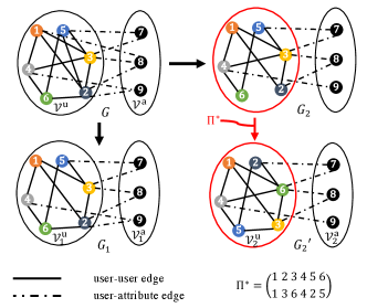
Base graph generation. We first generate a base graph $G$, whose vertex set $\mathcal{V}(G)$ consists of two disjoint sets, the user vertex set $\mathcal{V}^{\mathrm{u}}=\{1,2,\ldots,n\}$ and the attribute vertex set $\mathcal{V}^{\mathrm{a}}=\{n+1,n+2,\ldots,n+m\}$. There are two types of edges in the base graph $G$, the user-user edges (edges connecting a pair of users) and the user-attribute edges (edges connecting a user vertex and an attribute vertex). The user-user edges are generated independently and identically with probability $p$, and the user-attribute edges are generated independently and identically with probability $q$. Throughout this paper, we assume that $p=o(1)$ and $q=o(1)$. We write $i\stackrel{{\scriptstyle G}}{{\sim}}j$ if vertices $i$ and $j$ are connected in graph $G$.

Edge subsampling. From the base graph $G$, we obtain two correlated graphs $G_{1}$ and $G_{2}$ by subsampling the edges in $G$ independently. More specifically, we get $G_{1}$ and $G_{2}$ by independently including each user-user edge in $G$ with probability $s_{\mathrm{u}}$ and independently including each user-attribute edge with probability $s_{\mathrm{a}}$. Throughout this paper, we assume that $s_{\mathrm{u}}=\Theta(1)$ and $s_{\mathrm{a}}=\Theta(1)$.

Anonymization. From the $G_{2}$ generated as above, we get an anonymized graph $G_{2}^{\prime}$ by applying an unknown permutation $\Pi^{*}$ on the user vertices of $G_{2}$, where $\Pi^{*}$ is drawn uniformly at random from the set of all possible permutations on $\mathcal{V}^{\mathrm{u}}$. We use $\mathcal{V}_{2}^{\text{u}}$ to denote the user vertex set of $G_{2}^{\prime}$ and use $\mathcal{V}_{1}^{\text{u}}$ to denote the user vertex set of $G_{1}$. Finally, we remark that this subsampling process is a special case of an earlier described attributed Erdős–Rényi pair model in [1].

Exact alignment. Given an observable pair $(G_{1},G_{2}^{\prime})$, our goal is to recover the unknown permutation $\Pi^{*}$, which allows us to recover the original labels of user vertices in the anonymized graph $G_{2}^{\prime}$. We say exact alignment is achieved with high probability (w.h.p.) if $\lim_{n\rightarrow\infty}\mathsf{P}(\hat{\Pi}\neq\Pi^{*})=0$. It is worth mentioning that ${\mathsf{P}}(\hat{\Pi}\neq\Pi^{*})={\mathsf{P}}(\hat{\Pi}\neq\Pi^{*}|\Pi^{*}=\pi_{\text{id}})$ due to the symmetry among user vertices. Thus, we later assume without loss of generality that the underlying true permutation is the identity permutation.

Related random graph models. A closely related graph generation model is the correlated stochastic block model [20, 21, 22]. In this model, the base graph $G$ is instead generated from the stochastic block model, where vertices are grouped into latent blocks, and edges are formed between blocks with specific probabilities, capturing the underlying community structure in the network. The base graph $G$ is then subsampled into the two generated graphs $G_{1}$ and $G_{2}$. In the proposed attributed Erdős–Rényi graph pair models, users and attributes can be viewed as two communities in the correlated stochastic block model. However, a key distinction lies in the fact that the attributed Erdős–Rényi graph pair model specifies the correspondence between attributes in the two graphs, whereas the correlated stochastic block model does not disclose such information.

Another well-studied graph alignment model with side information is the seeded Erdős–Rényi graph pair model [11, 12, 13, 14], where we have access to part of the true correspondence between user vertices. To make a comparison between the seeded Erdős–Rényi graph pair model and the proposed model, here we describe the seeded Erdős–Rényi pair model $\mathcal{G}(N,\alpha,p,s)$ in detail. We first sample a base graph $G$ from the Erdős–Rényi graph on $N$ vertices with edge probability $p$. Then two correlated copies $G_{1}$ and $G_{2}$ are obtained by independently subsampling the edges in the base graph where each edge is preserved with probability $s$. The anonymized graph $G_{2}^{\prime}$ is obtained by applying an unknown permutation $\Pi^{*}$ on $G_{2}$, where $\Pi^{*}$ is drawn uniformly at random. Let $\mathcal{V}(G_{1})$ and $\mathcal{V}(G_{2}^{\prime})$ denote the vertex sets of $G_{1}$ and $G_{2}^{\prime}$ respectively. Then, a subset $\mathcal{V}_{s}\subset\mathcal{V}(G_{1})$ of size $\lfloor N\alpha\rfloor$ is chosen uniformly at random and we define the vertex pairs $\mathcal{I}_{0}=\{(v_{1},\Pi^{*}(v_{1})):v_{1}\in\mathcal{V}_{s}\}$ as the seed set. The graph pair $(G_{1},G_{2}^{\prime})$ together with the seed set $\mathcal{I}_{0}$ are given and the goal of the exact alignment is to recover the underlying permutation for the remaining vertices w.h.p.

Comparing the seeded Erdős–Rényi pair model and the attributed Erdős–Rényi pair model, we can see that the seed set and the attribute set both provide side information to assist the alignment of the remaining vertices. Nevertheless, there are two main differences between the two models. First, in the attributed Erdős–Rényi pair model, we allow different edge probabilities and subsampling probabilities for user-user edges and user-attribute edges, whereas in the seeded Erdős–Rényi pair model, the edge probability is identical for all edges and so is the subsampling probability. Second, while there are edges between seeds in seeded Erdős–Rényi pair model, there are no attribute-attribute edges in the attributed Erdős–Rényi pair model. However, it can be shown that the existence of edges between seeds has no influence on the information-theoretic limits for exact alignment in the seeded Erdős–Rényi pair model (see Lemma 1 in [23]). This further suggests that regarding the task of exact alignment, the information-theoretic limits on attributed graph alignment recover the information-theoretic limits on seeded Erdős–Rényi graph alignment if we specialize $p=q$ and $s_{\mathrm{u}}=s_{\mathrm{a}}$ in the attributed Erdős–Rényi pair model $\mathcal{G}(n,p,s_{\mathrm{u}};m,q,s_{\mathrm{a}})$.

Other notation. Our algorithms rely on exploring the neighborhood similarity of user vertices in $G_{1}$ and $G_{2}^{\prime}$. Here we introduce our notation of local neighborhoods. We define $\mathcal{N}_{1}^{\text{a}}(i)\triangleq\{j\in\mathcal{V}_{1}^{\text{a}}:i\stackrel{{\scriptstyle G_{1}}}{{\sim}}j\}$ as the set of attribute neighbors of a user vertex $i$ in $G_{1}$ and $\mathcal{N}_{2}^{\text{a}}(i)\triangleq\{j\in\mathcal{V}_{2}^{\text{a}}:i\stackrel{{\scriptstyle G_{2}^{\prime}}}{{\sim}}j\}$ as the set of attribute neighbors of a user vertex $i$ in $G_{2}^{\prime}$. For two user vertices $i$ and $j$ in the same graph, let $d(i,j)$ be the length of the shortest path connecting $i$ and $j$ via user-user edges. For a user vertex $i\in\mathcal{V}_{1}^{\text{u}}$, we define the set of $l$-hop user neighbors of vertex $i$ as $\mathcal{N}_{1}^{\text{u}}(i,l)\triangleq\{j\in\mathcal{V}_{1}^{\text{u}}:d(i,j)\leq l\}$ for any positive integer $l$. By convention, when $l=1$, we simply write $\mathcal{N}_{1}^{\text{u}}(i)\equiv\mathcal{N}_{1}^{\text{u}}(i,1)$. The quantities $\mathcal{N}_{2}^{\text{u}}(i,l)$ and $\mathcal{N}_{2}^{\text{u}}(i)$ are defined similarly for user vertices in $G_{2}^{\prime}$.

Reminder of the Landau notation.

In this section, we propose two polynomial-time algorithms for the attributed graph alignment problem. Their feasible regions are characterized in the following two theorems.

The proofs of Theorems 1 and 2 are deferred to Sections V and VI respectively.

In this section, we compare the feasible region in Theorems 1 and 2 to existing works. In Section IV-A, we compare the feasible region with the information-theoretic limits in [1]. It is shown that there still exists a gap between the feasible region of the proposed algorithms and the information-theoretic limit. In Section IV-B, we specialize the feasible region of the proposed algorithm to the context of seeded graph alignment problem, and compare the specialized feasible region to the information-theoretic limits as well as the best-known feasible regions by polynomial-time algorithms for exact alignment in literature given in [13] and [14]. It is shown that while having a gap to the information-theoretic limit, the proposed Algorithms AttrRich and AttrSparse achieves exact recovery in certain range of parameters that is unknown to be feasible by any existing efficient algorithms. In Section IV-C, we consider the bipartite alignment problem which is another special case. We show that the proposed Algorithm AttrRich provides an alternative polynomial-time algorithm to the theoretically optimal Hungarian Algorithm [24], with a slightly lower complexity.

References

• Zhang et al. [2021] N. Zhang, W. Wang, and L. Wang, “Attributed graph alignment,” in Proc. IEEE Internat. Symp. Inf. Theory, 2021, pp. 1829–1834.
• Pedarsani and Grossglauser [2011] P. Pedarsani and M. Grossglauser, “On the privacy of anonymized networks,” in Proc. Ann. ACM SIGKDD Conf. Knowledge Discovery and Data Mining (KDD), 2011, pp. 1235–1243.
• Cullina and Kiyavash [2016] D. Cullina and N. Kiyavash, “Improved achievability and converse bounds for Erdős-Rényi graph matching,” ACM SIGMETRICS Perform. Evaluation Rev., vol. 44, no. 1, p. 63–72, June 2016.
• Cullina and Kiyavash [2017] D. Cullina and N. Kiyavash, “Exact alignment recovery for correlated Erdős-Rényi graphs,” 2017. [Online]. Available: https://arxiv.org/abs/1711.06783
• Wu et al. [2022] Y. Wu, J. Xu, and S. H. Yu, “Settling the sharp reconstruction thresholds of random graph matching,” IEEE Transactions on Information Theory, vol. 68, no. 8, pp. 5391–5417, 2022.
• Dai et al. [2019] O. Dai, D. Cullina, N. Kiyavash, and M. Grossglauser, “Analysis of a canonical labeling algorithm for the alignment of correlated erdős-rényi graphs,” ACM SIGMETRICS Perform. Evaluation Rev., vol. 47, pp. 96–97, 12 2019.
• Ding et al. [2021] J. Ding, Z. Ma, Y. Wu, and J. Xu, “Efficient random graph matching via degree profiles,” Probability Theory and Related Fields, vol. 179, pp. 29–115, 2021.
• Fan et al. [2020] Z. Fan, C. Mao, Y. Wu, and J. Xu, “Spectral graph matching and regularized quadratic relaxations: Algorithm and theory,” in Proceedings of the 37th International Conference on Machine Learning, ser. Proceedings of Machine Learning Research, H. D. III and A. Singh, Eds., vol. 119.   PMLR, 13–18 July 2020, pp. 2985–2995.
• Mao et al. [2023a] C. Mao, M. Rudelson, and K. Tikhomirov, “Exact matching of random graphs with constant correlation,” Probability Theory and Related Fields, vol. 186, no. 1-2, pp. 327–389, 2023.
• Mao et al. [2023b] C. Mao, Y. Wu, J. Xu, and S. H. Yu, “Random graph matching at otter’s threshold via counting chandeliers,” in Proceedings of the 55th Annual ACM Symposium on Theory of Computing, 2023, pp. 1345–1356.
• Korula and Lattanzi [2014] N. Korula and S. Lattanzi, “An efficient reconciliation algorithm for social networks,” Proc. VLDB Endow., vol. 7, no. 5, p. 377–388, jan 2014.
• Yartseva and Grossglauser [2013] L. Yartseva and M. Grossglauser, “On the performance of percolation graph matching,” in Proceedings of the First ACM Conference on Online Social Networks, ser. COSN ’13.   New York, NY, USA: Association for Computing Machinery, 2013, p. 119–130. [Online]. Available: https://doi.org/10.1145/2512938.2512952
• Mossel and Xu [2020] E. Mossel and J. Xu, “Seeded graph matching via large neighborhood statistics,” Random Structures & Algorithms, vol. 57, no. 3, pp. 570–611, 2020.
• Shirani et al. [2017] F. Shirani, S. Garg, and E. Erkip, “Seeded graph matching: Efficient algorithms and theoretical guarantees,” in Proc. Asilomar Conf. Signals, Systems, and Computers, 2017, pp. 253–257.
• Zhang and Tong [2016] S. Zhang and H. Tong, “Final: Fast attributed network alignment,” in Proc. Ann. ACM SIGKDD Conf. Knowledge Discovery and Data Mining (KDD), ser. KDD ’16.   New York, NY, USA: Association for Computing Machinery, 2016, p. 1345–1354.
• Zhang and Tong [2019] ——, “Attributed network alignment: Problem definitions and fast solutions,” Proc. IEEE Trans. Knowl. Data Eng., vol. 31, no. 9, pp. 1680–1692, 2019.
• Zhou et al. [2021] Q. Zhou, L. Li, X. Wu, N. Cao, L. Ying, and H. Tong, Attent: Active Attributed Network Alignment.   New York, NY, USA: Association for Computing Machinery, 2021, p. 3896–3906.
• Yu [2023] S. H. Yu, “Matching in networks: Fundamental limits and efficient algorithms,” Ph.D. dissertation, Duke University, 2023.
• Mao et al. [2022] C. Mao, Y. Wu, J. Xu, and S. H. Yu, “Testing network correlation efficiently via counting trees,” arXiv preprint arXiv:2110.11816, 2022.
• Onaran et al. [2016] E. Onaran, S. Garg, and E. Erkip, “Optimal de-anonymization in random graphs with community structure,” in 2016 50th Asilomar Conference on Signals, Systems and Computers, 2016, pp. 709–713.
• Cullina et al. [2016] D. Cullina, K. Singhal, N. Kiyavash, and P. Mittal, “On the simultaneous preservation of privacy and community structure in anonymized networks,” arXiv preprint arXiv:1603.08028, 2016.
• Lyzinski et al. [2015] V. Lyzinski, D. E. Fishkind, M. Fiori, J. T. Vogelstein, C. E. Priebe, and G. Sapiro, “Graph matching: Relax at your own risk,” IEEE transactions on pattern analysis and machine intelligence, vol. 38, no. 1, pp. 60–73, 2015.
• Zhang et al. [2023] N. Zhang, Z. Wang, W. Wang, and L. Wang, “Attributed graph alignment,” 2023. [Online]. Available: https://arxiv.org/abs/2102.00665
• Kuhn and Yaw [1955] H. W. Kuhn and B. Yaw, “The Hungarian method for the assignment problem,” Naval Res. Logist. Quart, pp. 83–97, 1955.
• Munkres [1957] J. Munkres, “Algorithms for the assignment and transportation problems,” Journal of the Society for Industrial and Applied Mathematics, vol. 5, no. 1, pp. 32–38, 1957. [Online]. Available: http://www.jstor.org/stable/2098689
• Hoeffding [1963] W. Hoeffding, “Probability inequalities for sums of bounded random variables,” Journal of the American Statistical Association, vol. 58, no. 301, pp. 13–30, 1963.
• Ash [1990] R. Ash, Information Theory, ser. Dover books on advanced mathematics.   Dover Publications, 1990.