On the feasibility of deriving pseudo-redshifts of gamma-ray bursts from two phenomenological correlations
Abstract
Accurate knowledge of gamma-ray burst (GRB) redshifts is essential for studying their intrinsic properties and exploring their potential application in cosmology. Currently, only a small fraction of GRBs have independent redshift measurements, primarily due to the need of rapid follow-up optical/IR spectroscopic observations. For this reason, many have utilized phenomenological correlations to derive pseudo-redshifts of GRBs with no redshift measurement. In this work, we explore the feasibility of analytically deriving pseudo-redshifts directly from the Amati and Yonetoku relations. We simulate populations of GRBs that (i) fall perfectly on the phenomenological correlation track, and (ii) include intrinsic scatter matching observations. Our findings indicate that, in the case of the Amati relation , the mathematical formulation is ill-behaved so that it yields two solutions within a reasonable redshift range . When realistic scatter is included, it may result in no solution, or the redshift error range is excessively large. In the case of the Yonetoku relation, while it can result in a unique solution in most cases, the large systematic errors of the redshift calls for attention, especially when attempting to use pseudo redshifts to study GRB population properties.
1 Introduction
Gamma-ray bursts (GRBs) rank among the most luminous explosions in the Universe. Their isotropic and extragalactic origins were firmly established by the Burst and Transient Source Experiment (BATSE) onboard the Compton Gamma Ray Observatory (Meegan et al., 1992); due to their extraordinary brightness, they have been detected up to a redshift (Cucchiara et al., 2011). Thus, GRBs stand as a potential candidate to perform cosmological studies (Amati & Valle, 2013). GRBs have traditionally been categorized by the duration of their prompt emission. Short-duration GRBs (SGRBs) are defined as those with seconds, while long-duration GRBs (LGRBs) have seconds; It is generally believed that the origin of SGRBs is attributed to the merger of binary compact objects, whereas LGRBs are associated with the deaths of massive stars (Zhang et al., 2009; Berger, 2014). However, this simple dichotomy of long versus short may not fully capture the complexity and intricacies of GRBs, since a subclass of GRBs have been found to exhibit properties of both LGRBs and SGRBs (Norris & Bonnell, 2006; Yi et al., 2023; Wang et al., 2024; Yi et al., 2024; Zhang, 2024). Moreover, using a phenomenological classification scheme based on , which depends on the detector’s energy band, can also lead to contradictory results between different detectors observing the same GRB (Bromberg et al., 2013). Zhang (2006) proposes a more physical classification scheme, where GRBs are divided into Type-I (merger origin) and Type-II (collapsar origin) categories, based on their progenitor; while it may not always be possible to determine the progenitor, GRBs exhibiting characteristics of both types can be categorized based on whether the majority of its properties align more closely with a merger or core collapse scenario.
In recent decades, GRBs have been found to exhibit various phenomenological correlations among parameters of the prompt emission. Among these are two robust correlations which correlate the spectral peak energy (in the spectrum), , to isotropic energy (Amati et al., 2008), and isotropic peak luminosity (Yonetoku et al., 2004), i.e.,
| (1) |
and
| (2) |
There exists two distinct tracks for LGRBs and SGRBs in (Amati) space, with SGRBs forming a parallel track above LGRBs, due to their lower energy output (See Fig.1). This may be attributed to their shorter durations. However, in – (Yonetoku) parameter space, there exists no significant separation between LGRBs and SGRBs.
The origin of these correlations remains a topic of active debate. While some have attributed them as being an artifact of instrumental selection biases (Band & Preece, 2005), several studies have quantified the impact of selection biases and concluded that, although selection effects may influence the slope and scatter, they cannot fully account for the existence of the spectral energy correlations. Further evidence for the Amati and Yonetoku correlations comes from the discovery of an relationship that appears within individual bursts (Liang et al., 2004; Frontera et al., 2012). Notwithstanding the uncertainties in the underlying physics, many have considered their potential utility in deriving “pseudo-redshifts” (Yonetoku et al., 2004; Dainotti et al., 2011; Tan et al., 2013; Tsutsui et al., 2013; Deng et al., 2023), which would be particularly vital for population studies. For example, Zhang & Wang (2018) applied the Yonetoku relation to constrain the luminosity function and formation rate of SGRBs, while others, such as Wanderman & Piran (2015) and Paul (2018), have investigated the evolution of the luminosity function in depth. Given that Fermi-GBM has amassed a dataset of over 2,400 GRB detections since its launch (Poolakkil et al., 2021), we believe it is pertinent to evaluate the viability of using these correlations for deriving pseudo-redshifts.
In this study, we test the feasibility of using the Amati and Yonetoku relations to analytically derive pseudo-redshifts by utilizing a synthetic catalogue of GRBs and comparing the inferred psuedo-redshifts (henceforth denoted as ) to their true, generated redshift . We mainly consider the case for LGRBs as they have traditionally been used for cosmological studies; however, we also provide some analysis for SGRBs in the Discussion. The paper is organized as follows: section 2 describes our detailed simulation process; in section 3, we summarize our results, and section 4 offers a summary and discussion.

2 Methods
The Amati correlation is defined in terms of two intrinsic (i.e., rest-frame) quantities: the peak energy and the isotropic energy , for a given redshift . The intrinsic parameters and are related to their observed counterparts through
| (3) |
and
| (4) |
where is the fluence, is the k-correction (which we take as , due to the wide energy coverage of Fermi-GBM), and is the luminosity distance, i.e.,
| (5) |
We adopt the Planck18 cosmology, assuming a flat CDM universe with and as reported by Aghanim et al. (2020). Holding and fixed for a given burst, and allowing to vary continuously (over ), we trace out a continuous curve in the plane. We refer to this locus of points as
| (6) |
Geometrically, it is a parametric curve where the running parameter is . We next compare to the best-fit Amati line; any intersection between and this correlation line corresponds to a candidate “pseudo-redshift” : that is, a redshift for which the observed values place the burst exactly on the Amati relation.
We fit the Amati parameters to the LGRB sample of Lan et al. (2023), finding and We first simulate a population of 100 GRBs that perfectly obey this best-fit Amati line 111All the relevant codes in this paper can be accessed from the GitLab repository </> . Specifically, we first draw values from the observed distribution of Lan et al. (2023) and sample the “true” redshift for each GRB from a typical LGRB formation rate (Salvaterra & Chincarini, 2007):
| (7) |
where is the metallicity-convolved efficiency function (Kewley & Kobulnicky, 2005)
| (8) |
is the star formation rate from Li (2008) and we take the normalization factor . For each simulated burst, we set
and then compute its observed fluence and observed peak energy via Equations. 3 and 4.
Thus, each simulated GRB is assigned both intrinsic parameters and observed parameters . Finally, to infer its pseudo-redshift, we construct the parametric curve and find any intersection(s) with the Amati line. The resulting solution(s) can then be compared to the known “true” . Reliable distance indicators must yield only a single redshift solution within a reasonable redshift range, and so we wish to see if the Amati relation can yield a unique solution for each GRB, given its observed spectral peak energy and fluence . Next, we add intrinsic scatter to the simulated data, based on our measured dispersion of = 0.30 on the data of Lan et al. (2023), where we attempt to gauge the statistics of with a simulated catalogue of 500 GRBs; this dispersion defines an upper and lower boundary around the best-fit Amati relation, forming the uncertainty region . For each simulated GRB, we determine its 1 redshift range by finding where the parametric curve intersects .


In the case of the Yonetoku relation, the intrinsic luminosity is given by
| (9) |
where is the observed flux. Since we are substituting with luminosity, the GRB parametric curve in Yonetoku parameter space takes on a distinct functional form with respect to than ; in this case, each simulated GRB in Yonetoku parameter space is characterized by the parameters and warrants a separate investigation. We follow a similar procedure outlined for the Amati relation when assigning the intrinisic parameters of the simulated GRBs, and dispersion according to = 0.25 (Ghirlanda et al., 2005), which defines the Yonetoku uncertainty band . We take to be 0.625 , and to be -30.22 taken from literature (Yonetoku et al., 2010) 222From Yonetoku et al. (2010),
Thus, = , and = . We sample the luminosities from a simple lognormal distribution . Note that the choice of luminosity function does not alter the key results, because the functional form of —and hence the geometry of its intersection with the Yonetoku correlation—remains unchanged. Consequently, only the relative weighting of the parameter space is affected, not the overall behavior of solutions.
3 Results
3.1 Amati Relation
In the top left panel of Figure 2, we display two example curves of GRBs simulated without scatter (assuming perfect Amati relation) overlaid on the best-fit Amati line within the Amati parameter space. It is evident that these GRBs have double intersections with the Amati line. In fact, unless the parametric curve is exactly tangent to the Amati line—which occurs only at a specific redshift —there will be two redshift solutions for each GRB, one with and another with . We derive an expression for , which is dependant on the Amati slope (see Appendix):
| (10) |
In the bottom left panel of Fig. 2, we show that analytically solving the Amati relation yields two solutions, with (i) and (ii) ; the two solution branches of and intersect at , as predicted by Eq 10 (See left panel of Figure 6 in the appendix). The condition that determines whether the Amati relation is “ill-behaved” in the physical redshift interval depends on how steep is. Specifically, one can require ensuring every parametric curve to admit a single solution rather than two. This translates to a limiting slope , significantly larger than the best-fit value currently measured (see the left panel of Fig. 6) in the appendix
When we incorporate intrinsic scatter into the simulated GRBs as previously described, the curves will either have no solution, a single solution, or double solution. As a direct corollary of Eq 10, we see that taking the redshift at which is closest to the mean Amati line for those curves which do not intersect the Amati line will always result in the same redshift, . The curves which yield only a single solution (about 34% of the sample) will always have (see Fig 7 in appendix).
When we consider the intersection of with the Amati dispersion area , the curves would either have no crossings (10%) , single crossings, or double crossings (8%) . In the bottom right panel of Fig. 2, we plot the confidence intervals against , including both GRBs with single crossings or double crossings. Clearly, even with the 1 uncertainty band, the uncertainty range of is around the same order of magnitude as the redshift range of interest, and in fact often extends beyond . There exists no correlation between and . Note that the case of single crossings here is intrinsically different from the case of with a single intersection (at ) when simulated without scatter.


3.2 Yonetoku Relation
Because is more sensitive to redshift than , the parametric curve does not intersect the correlation line multiple times within . As a result, each burst yields a unique solution for (see Fig. 3). . With the same line of reasoning adopted for the case of the Amati relation, we can obtain a threshold slope for which the Yonetoku relation would no longer always yield a unique solution within , through
| (11) |
where we find that the condition of being ill-behaved is satisfied for , well below the uncertainty range for (See right panel of Fig 6 in Appendix). Therefore, the Yonetoku relation is always well behaved and provides a unique redshift solution within . When intrinsic scatter is added to , we find that about 5% of GRBs do not intersect the Yonetoku line. In the bottom left panel of Fig. 4, we plot vs . It is evident that the vs trend is highly sensitive to the intrinsic scatter of the sample; we obtain a pearson correlation coefficient of , indicating little predictive power.
In the bottom right panel of Figure 4, we show vs , found from the intersection of with the yonetoku dispersion area ; unlike in the case of the Amati relation, we do not find any curves with double crossings, and a small fraction () of curves have no crossings. Nonetheless, the confidence bands are excessively large, often extending well beyond . We cap to 20.
4 Summary & Discussion
In this paper, we examine the feasibility of analytically obtaining pseudo-redshifts using two well-known phenomenological correlations of the prompt emission, which have become the de facto method for this purpose. With the aid of a synthetic catalogue of GRBs, we find this practice to be untenable for the following reasons:
-
•
Analytically solving for from the best fit Amati relation always results in two solutions, which are both within a physical range (except in the case of ). The Amati relation can be practically well behaved over if the Amati slope , well above the uncertainty range of . Intrinsic scatter would not salvage the situation; if intrinsic scatter is added, there would either be (i) two solutions, (ii) one solution, or (iii) no solution. In the case of no solution, taking the point on closest to the mean Amati track would only yield a constant , as a corollary of Equation 10. In the case of a single solution, it is easy to see that in all cases , and hovers around a constant value. Therefore, the Amati relation fails at a fundamental level and cannot be reliably used as a distance indicator
-
•
Although the Yonetoku relation results in a unique solution for , the intrinsic scatter leads to there being no solution for about 5% simulated GRBs and little predictive power of .
-
•
Incorporating the confidence areas and would yield excessively large error bands for for both the Amati and Yonetoku relations.
We have not simulated GRBs with uncertainty bands in and , so in practice, we would expect even larger uncertainties in if the uncertainties of fluence and peak energy are accounted for. In order to check whether the redshift distribution of the simulated GRB population will change the above analysis on the Yonetoku relation, we repeat the analysis with a different redshift distribution, a density evolved rate, as proposed in Lan et al, ie, , with , which places more GRBs at higher redshifts Lan et al. (2019). In this case, the strength of the vs correlation decreases to , and the curves of about 20% of LGRBs would not intersect the Yonetoku line, and hence have no solution. In the vs. plots shown in Figure 4, not only is the scatter around the line quite large, but the confidence intervals for individual are also very wide—exceeding 2.5 for GRBs with . For LGRBs, the 1 confidence interval of (upper limit capped at 10) averages to 4.19, which is broader than the characteristic width () of the metallicity-convolved GRB rate distribution. It is critical to emphasize again that this result is without considering for errors in measurements of fluence and peak energy. Such high uncertainties of the inferred (significantly larger than the width of distribution of the population) calls into question the feasibility of any population studies which aim to infer distributions directly from pseudo-redshifts; for instance, it would be difficult to obtain any meaningful constraints on our understanding between the correlation of LGRBs and the cosmic star formation history, the characteristic delay time, or the luminosity function.
In this work, we have assumed a k-correction factor of 1; in reality, the curves of and would be slightly modified. Zegarelli et al. (2022) found the k-correction distribution of GRBs detected by Fermi-GBM to be highly skewed towards 1, with a median value of 1.12 and a mean value of 1.27, and with a maximum value of an outlier at 4. Therefore, although in principle would increase with , the effect would be negligible due to the wide energy coverage of Fermi-GBM. In fact, Paul (2018) demonstrated that by assuming Fermi-GBM’s GRBs follow the Band function and averaging the low- and high-energy indices and , the average spectral shape detected by Fermi-GBM yields a k-correction below 1.5 even at .
4.1 SGRBs
Although most cosmological uses of GRBs focus on long-duration bursts, we have also briefly examined the case of SGRBs, whose redshift distribution is expected to peak at lower . With regards to the Amati relation, since the slope for SGRBs is also below the limiting value for a unique solution, our conclusion for long GRBs extends equally to short GRBs in this context. With regards to the Yonetoku relation, we sample the SGRBs from a BNS merger rate density (see appendix). Assuming Gyr, we obtain a correlation coefficient of for vs. , and the average 1 sigma confidence intervals of (capping the upper limit to 10 ) is 3.16, which greatly exceeds the delay time-scale (). In the case of = 1 Gyr, we find for vs. and the average 1 sigma confidence intervals of is 3.57.

4.2 Concluding Remarks
Our findings underscore the inherent difficulty in analytically solving for redshifts using phenomenological GRB correlations as distance indicators for both individual GRBs and population studies. Nevertheless, it is important to stress that these correlations, when combined with other observational information or advanced statistical/machine-learning frameworks, may still hold promise for constraining population distributions (e.g., luminosity functions, formation rates). For instance, Bayesian hierarchically informed methods or multi-parameter regressions leveraging detailed spectral shapes, afterglow properties, or prompt light-curve features could help refine pseudo-redshift estimates. In fact, recent studies have incorporated machine learning with great success in deriving pseudo-redshifts; (See, for example, Dainotti et al., 2024; Aldowma & Razzaque, 2024). In the study of Aldowma & Razzaque (2024), for instance, the models included not only the key parameters of fluence, flux, and peak energy, but also additional spectral features, such as the low and high spectral indices of the Band function. This broader set of input variables allows machine learning approaches to identify complex, non-linear relationships that may not be immediately apparent in traditional regression-based methods. We stress that machine learning does not override the foundational limitations we present here, but instead provides a complementary way to address them by utilizing a wider range of observational data. Hence, we believe that the extensive data collected by Fermi-GBM still retains potential in this regard.
We have not considered other phenomenological correlations of the prompt emission, such as (Ghirlanda) relation (Ghirlanda et al., 2004), (Firmani) relation (Firmani et al., 2006), or those of the afterglow, such as the (Dainotti) relation (Dainotti et al., 2008) and (Liang-Zhang) relation (Liang & Zhang, 2005). Nonetheless, if any such correlations are to be used as “distance indicators”, they must (i) yield a unique solution within a physical redshift range, and (ii) be tight enough to have a predictive power of statistical significance and yield reasonable error bands.
References
- Aghanim et al. (2020) Aghanim, N., Akrami, Y., Ashdown, M., et al. 2020, Astronomy & Astrophysics, 641, A6
- Aldowma & Razzaque (2024) Aldowma, T., & Razzaque, S. 2024, Monthly Notices of the Royal Astronomical Society, 529, 2676
- Amati et al. (2008) Amati, L., Guidorzi, C., Frontera, F., et al. 2008, MNRAS, 391, 577, doi: 10.1111/j.1365-2966.2008.13943.x
- Amati & Valle (2013) Amati, L., & Valle, M. D. 2013, International Journal of Modern Physics D, 22, 1330028, doi: 10.1142/S0218271813300280
- Band & Preece (2005) Band, D. L., & Preece, R. D. 2005, Astrophys. J., 627, 319, doi: 10.1086/430402
- Berger (2014) Berger, E. 2014, Annual Review of Astronomy and Astrophysics, 52, 43
- Bromberg et al. (2013) Bromberg, O., Nakar, E., Piran, T., et al. 2013, The Astrophysical Journal, 764, 179
- Cucchiara et al. (2011) Cucchiara, A., Levan, A. J., Fox, D. B., et al. 2011, The Astrophysical Journal, 736, 7
- Dainotti et al. (2008) Dainotti, M. G., Cardone, V. F., & Capozziello, S. 2008, Monthly Notices of the Royal Astronomical Society: Letters, 391, L79
- Dainotti et al. (2011) Dainotti, M. G., Fabrizio Cardone, V., Capozziello, S., Ostrowski, M., & Willingale, R. 2011, ApJ, 730, 135, doi: 10.1088/0004-637X/730/2/135
- Dainotti et al. (2024) Dainotti, M. G., Taira, E., Wang, E., et al. 2024, The Astrophysical Journal Supplement Series, 271, 22
- Deng et al. (2023) Deng, C., Huang, Y.-F., & Xu, F. 2023, The Astrophysical Journal, 943, 126
- Firmani et al. (2006) Firmani, C., Ghisellini, G., Avila-Reese, V., & Ghirlanda, G. 2006, Monthly Notices of the Royal Astronomical Society, 370, 185
- Frontera et al. (2012) Frontera, F., Amati, L., Guidorzi, C., Landi, R., et al. 2012, The Astrophysical Journal, 754, 138
- Ghirlanda et al. (2005) Ghirlanda, G., Ghisellini, G., Firmani, C., Celotti, A., & Bosnjak, Z. 2005, Monthly Notices of the Royal Astronomical Society: Letters, 360, L45
- Ghirlanda et al. (2004) Ghirlanda, G., Ghisellini, G., & Lazzati, D. 2004, The Astrophysical Journal, 616, 331
- Kewley & Kobulnicky (2005) Kewley, L., & Kobulnicky, H. A. 2005, in Starbursts: From 30 Doradus to Lyman Break Galaxies (Springer), 307–310
- Lan et al. (2019) Lan, G.-X., Zeng, H.-D., Wei, J.-J., & Wu, X.-F. 2019, Monthly Notices of the Royal Astronomical Society, 488, 4607
- Lan et al. (2023) Lan, L., Gao, H., Li, A., et al. 2023, The Astrophysical Journal Letters, 949, L4
- Li (2008) Li, L.-X. 2008, Monthly Notices of the Royal Astronomical Society, 388, 1487
- Liang & Zhang (2005) Liang, E., & Zhang, B. 2005, The Astrophysical Journal, 633, 611
- Liang et al. (2004) Liang, E. W., Dai, Z.-G., & Wu, X. F. 2004, Astrophys. J. Lett., 606, L25, doi: 10.1086/421016
- Madau & Dickinson (2014) Madau, P., & Dickinson, M. 2014, Annual Review of Astronomy and Astrophysics, 52, 415
- Meegan et al. (1992) Meegan, C., Fishman, G., Wilson, R., et al. 1992, Nature, 355, 143
- Norris & Bonnell (2006) Norris, J. P., & Bonnell, J. T. 2006, The Astrophysical Journal, 643, 266
- Paul (2018) Paul, D. 2018, Monthly Notices of the Royal Astronomical Society, 473, 3385
- Poolakkil et al. (2021) Poolakkil, S., Preece, R., Fletcher, C., et al. 2021, The Astrophysical Journal, 913, 60
- Salvaterra & Chincarini (2007) Salvaterra, R., & Chincarini, G. 2007, The Astrophysical Journal, 656, L49
- Tan et al. (2013) Tan, W.-W., Cao, X.-F., & Yu, Y.-W. 2013, ApJ, 772, L8, doi: 10.1088/2041-8205/772/1/L8
- Tsutsui et al. (2013) Tsutsui, R., Yonetoku, D., Nakamura, T., Takahashi, K., & Morihara, Y. 2013, MNRAS, 431, 1398, doi: 10.1093/mnras/stt262
- Vitale et al. (2019) Vitale, S., Farr, W. M., Ng, K. K., & Rodriguez, C. L. 2019, The Astrophysical Journal Letters, 886, L1
- Wanderman & Piran (2015) Wanderman, D., & Piran, T. 2015, MNRAS, 448, 3026, doi: 10.1093/mnras/stv123
- Wang et al. (2024) Wang, C.-W., Tan, W.-J., Xiong, S.-L., et al. 2024, arXiv e-prints, arXiv:2407.02376, doi: 10.48550/arXiv.2407.02376
- Yi et al. (2024) Yi, S.-X., Seyit Yorgancioglu, E., Xiong, S. L., & Zhang, S. N. 2024, arXiv e-prints, arXiv:2411.16174, doi: 10.48550/arXiv.2411.16174
- Yi et al. (2023) Yi, S. X., Wang, C. W., Shao, X. Y., et al. 2023, arXiv e-prints, arXiv:2310.07205, doi: 10.48550/arXiv.2310.07205
- Yonetoku et al. (2004) Yonetoku, D., Murakami, T., Nakamura, T., et al. 2004, The Astrophysical Journal, 609, 935
- Yonetoku et al. (2010) Yonetoku, D., Murakami, T., Tsutsui, R., et al. 2010, Publications of the Astronomical Society of Japan, 62, 1495
- Zegarelli et al. (2022) Zegarelli, A., Celli, S., Capone, A., et al. 2022, Physical Review D, 105, 083023
- Zhang (2006) Zhang, B. 2006, Nature, 444, 1010
- Zhang (2024) Zhang, B. 2024, arXiv e-prints, arXiv:2501.00239, doi: 10.48550/arXiv.2501.00239
- Zhang et al. (2009) Zhang, B., Zhang, B.-B., Virgili, F., et al. 2009, The Astrophysical Journal, 703, 1696
- Zhang & Wang (2018) Zhang, G. Q., & Wang, F. Y. 2018, ApJ, 852, 1, doi: 10.3847/1538-4357/aa9ce5
Appendix A Derivation of Tangent Redshift
The Amati line is given by
| (A1) |
where is the slope of the Amati relation and is the intercept. in space is parameterized by
| (A2) |
and
| (A3) |
Lemma: The point on closest to the amati line for curves with no intersection occurs when the slope of in space matches the slope of the Amati line, .
We first need to compute the derivatives of with respect to :
| (A4) |
and
| (A5) |
We need to find the redshift at which the Amati slope and the derivative of match:
| (A6) |
Hence:
| (A7) |
since is a constant. It is easy to see that in the case of the Yonetoku relation, this becomes:
| (A8) |
We plot Equation A7 in Figure 6 (left), and Equation A8 in Figure 6 (right). It is clear that is at the midpoint of the intersection range between Equation A7 and the LGRB Amati slope uncertainty. The Yonetoku and Amati relations results unique solutions within for slopes which satisfy . Clearly the observed slopes of both relations indicate that the Yonetoku relation is well-behaved (resulting unique solution), but the Amati relation is not.
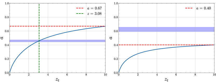
Figure 7 illustrates the case where the curves have only one solution when intrinsic scatter is introduced. This can be easily explained by noting that represents the highest possible redshift solution for curves that intersect the Amati line only once.


Appendix B The redshift distribution when simulating the population of sGRBs
We assume the SGRBs to follow the Binary Neutron Star (BNS) merger rate. The differential BNS merger rate as function of redshift , can be expressed in terms of the volumetric total BNS merger rate density in the source frame as
| (B1) |
where is the differential comoving volume. We adopt the Parametrization by Vitale et al. (2019) and take as:
| (B2) |
where is the non-normalized Madau-Dickinson star formation rate:
| (B3) |
with , , (Madau & Dickinson, 2014), and is the probability that a BNS system merges at given its formation at . This is the distribution of delay times, which has the form:
| (B4) |
Here, and are the look back time as a function of and , respectively. is the characteristic delay time. We sample SGRBs assuming a = 3 Gyr and 1 Gyr, and perform the same statistics as in section 3.2 . In Figure 8, we only show the results for the case of = 3 Gyr, as it is skewed towards smaller redshifts compared to the case of = 1 Gyr (See Figure 5).

