On the Energy Spectrum of Non-Newtonian Turbulence
Abstract
The goal of this paper is to propose a theoretical framework to study homogeneous and isotropic turbulence in a viscoelastic fluid, regarded as a perturbation of a Newtonian incompressible fluid, where the fluid relaxation time, or else the Weissenberg number, plays the role of small parameter. We use a Martin-Siggia-Rose framework to obtain a formal expression for the velocity correlation function of the non-Newtonian flow, and we expand this formal expression to linear order in the relaxation time. The coefficients in this expansion are correlation functions of the base Newtonian flow. We do not derive these correlations, instead we replace them by their values according to K41 theory, which could be regarded as an extreme form of renormalization. While substantial work will be necessary to validate the model against numerical and experimental data, preliminary results are encouraging.
I Introduction
The goal of this paper is to propose a theoretical framework for studying turbulent flows in situations beyond K41 theory [1, 2, 3] yet connected to it. The example we discuss is the spectrum of velocity fluctuations in homogeneous, isotropic turbulence of viscoelastic fluids [4, 5, 6, 7, 8, 9, 10, 11, 12], which reduce to Newtonian incompressible fluids when the relaxation time is taken to . Another example, closely connected to the first, see Appendix A, is the turbulent flow of a relativistic viscous fluid [13, 14], which becomes a Non-Newtonian fluid when the speed of light .
The basic idea is to formulate the problem within a Martin-Siggia-Rose (MSR) framework [15, 16, 17, 18, 19, 20]. In this approach, the Schwinger-Dyson equations for the causal response and the velocity correlations are derived from an effective action (EA) [21, 22, 23, 24, 25, 26, 27], which has a formal expression as a path integral over velocity and stress tensor fluctuations (details are provided in Section II). We then expand this formal expression in powers of the relaxation time (or its dimensionless equivalent, the Weissenberg number). The coefficients in this expansion can be written in terms of correlation functions in the base Newtonian flow. We do not derive these correlations from the MSR EA itself; instead, we substitute them with convenient ansätze suggested by K41 theory. This will allow us to sidestep some known criticisms of the MSR formalism in the literature [28, 29, 30, 31, 32, 33]. We discuss this strategy in the Final Remarks Section V; for the time being, we simply propose it as a matter of expediency.
Concretely, we begin by assuming that the Navier-Stokes equations (NSE) provide the “bare” description of homogeneous, isotropic turbulence in a Newtonian incompressible fluid. Then we perturb the NSE by adding non-Newtonian terms in the fluid stress tensor [34, 35, 36, 37]. The perturbation we consider arises in models of polymeric solutions [38, 39, 40, 41, 42, 43]. In Appendix A we show that this model also describes the non-relativistic limit of a conformal fluid [44, 45, 46]. We then work out the first order correction to the spectrum from the perturbed EA. We thus find a concrete analytical expression for the velocity correlation function of the viscoelastic flow, see eq. (56) below. Validating this expression against numerical and experimental data is a massive undertaking; preliminary comparisons at moderate Reynolds numbers and low Weissenberg numbers, such as the data presented in [10], are encouraging.
This paper is organized as follows. Next section II presents the basic notations and the equations of the fluid, both the NSE and the perturbed one. To make the work self-contained, we include an introduction to the MSR approach and the EA therefrom. We show how to derive the correlation functions from the EA and develop their perturbative expansion. In this Section we have adopted a highly compressed notation that best displays the structure of the problem, but we return to a more natural notation in the remaining Sections.
In section III we proceed to compute the kernels necessary to write down the perturbed Schwinger-Dyson equations, solve for the causal response function and finally derive the analytical expression for the spectrum of velocity correlations eq. (56), which is the main result of this paper. We begin with a brief review of the correlations in K41 theory. While this contains no new material, it is convenient to have all the basic formulae in one place.
In section IV we introduce the overall velocity scale (see eq. (57)) and the Taylor microscale (see eq. (58)) [47]. This allows us to define two dimensionless numbers, Reynolds number and Weissenberg number (see eqs. (59) and (60)) [37], which make it much easier to compare our results with the literature. We conclude with some brief final remarks in section V.
The paper includes four appendices. In Appendix A we show how the model in Section II describes the nonrelativistic limit of a conformal fluid. In Appendix B we discuss how to account for the random Galilean invariance [48, 49, 50, 51, 52] of the NSE in the EA formalism. This subject, which we left out of the main text for simplicity, has deep implications for the development of the theory. Appendixes Cand D contain some technical details.
II The model
The model is represented by the equations
| (1) |
| (2) |
where is the incompresible fluid velocity, is the stress tensor, is the pressure, is the constant fluid mass density, is the shear tensor
| (3) |
and is the kinematic viscosity. When at fixed we get an ordinary Newtonian fluid. When , the derivative terms in the second of eqs. (1) add up to the upper convected derivative of [37]. When it reduces to a material derivative, which is the case that describes the nonrelativistic limit of a conformal fluid, see Appendix A. In this note we shall assume .
We note that the right hand side of equations (1) ought to display stochastic sources necessary to put the fluid in motion. However, since we wish to work in the regime where fluid fluctuations are self-sustained, we shall not consider these sources explicitly.
To be able to derive equations (1) from a variational principle we introduce Lagrange multipliers and such that , and write
| (4) |
We delete the pressure term from , since it integrates to zero anyway.
II.1 The MSR EA
We see that the action functional eq. (4) depends on four different fields, the physical fields and and the auxiliary fields and . This diversity makes for a rather complex field theory.
To avoid unnecessary complications, we shall adopt an scheme based on three levels of description. Eqs. (1) and (4) belong to the first level, where we treat both physical and auxiliary fields as distinct. In the second level, however, we drop this distinction and gather together the physical fields into a single string , and similarly the auxiliary fields into a string . For higher compression, in the third level of description we regard all variables as components of a single object . In the second and third levels space-time indexes are included into the indexes and we apply Einstein’s convention to sums over indexes, both discrete and continuous.
Given an action we define a generating functional
| (5) |
were the are a string of external sources. Differentiation yields the mean fields
| (6) |
We shall work under conditions where symmetry forces all background fields to zero, namely homogeneous, isotropic turbulence. Further differentiation produces the higher cumulants, in particular the two-point correlations
| (7) |
where we are already using that the mean fields vanish. It is convenient to choose the mean fields, rather than the sources, as independent variables. To achieve this, we introduce the effective action as the Legendre transform of the generating functional
| (8) |
whereby we get the equations of motion for the mean fields
| (10) |
denotes the identity operator in the corresponding functional space. Similarly, from eq. (9) we get
| (11) |
These are the Schwinger-Dyson equations of the theory. From either of these equations we can derive the two-point correlations from the effective action.
II.2 Auxiliary and physical fields
We will now elaborate on the analysis above by distinguishing physical fields from auxiliary fields . We also distinguish the external sources coupled to physical fields from the sources coupled to auxiliary fields. The action eq. (4) is written as
| (12) |
The equations of motion are causal and we assume ([81])
| (13) |
We may choose the constant to be . The generating functional eq. (5) is expanded into
| (14) |
Observe that
| (15) |
identically, so all the expectation values of products of auxiliary fields vanish. Eq. (10) becomes
| (16) |
This implies that and are non singular, since
| (17) |
and then it must be
| (18) |
when the mean auxiliary fields vanish.
The correlations of type are the response functions of the theory. Once they are found, the physical correlations follow from
| (19) |
The second derivatives are the so-called “noise kernels” [22]
II.3 Computing the EA with the background field method
According to the usual rule [22], the EA is the classical action plus a “quantum correction”
| (20) |
To compute , we split all fields into a background value plus a fluctuation etc., expand the action eq. (4) and discard terms independent or linear in the fluctuations. Then
| (21) |
where is just the action eq. (4) evaluated on the fluctuation fields. is linear on the background fields and quadratic on the fluctuation fields. The sources enforce the constraints that the expectation value of the fluctuations vanish. For this reason, all one-particle insertions in the diagrammatic evaluation of the effective action cancel out, and it is enough to consider one-particle irreducible graphs only. We shall no longer write the sources explicitly, they are assumed to be included into .
We normalize the integration measure so that
| (22) |
So that . Then we find
| (23) |
Taking one more derivative
| (24) |
Expanding
| (25) |
then to first order in we have
| (26) | |||||
where
| (27) |
In computing the path integral only one-particle irreducible graphs should be considered.
The point of this analysis is that the expectation values in eq. (26) are computed at , that is, for a Newtonian theory. We shall not attempt to derive them from the path integral representation of , but rather assume that they take values that are consistent with K41 theory. We shall come back to discussing the validity of this procedure in the final remarks.
III Perturbative energy spectrum
In this Section we shall derive the energy spectrum to first order in , which will be evaluated in next Section IV. It is convenient to first review the response function and noise kernel in the K41 theory, which will be used later to build the corresponding kernels for viscoelastic flow.
III.1 Response and noise kernels in K41 theory
The K41 theory is built on the observation that turbulent fluctuations are non-Gaussian, with skewness
| (28) |
This is the so-called Kolmogorov’s law ([3]). The dynamically generated scale has dimensions of . It measures the transport of energy accross the turbulent cascade because of nonlinear interactions.
The K41 theory recognizes three flow regimes. There is a scale , basically the linear dimension of the flow, where energy is being injected. This scale and larger wavelengths form the “creation range”. Out of and the molecular viscosity we can form the Kolmogorov scale
| (29) |
At smaller length scales the flow is dominated by viscosity. This is the dissipation range.
From to we are in the inertial range, where is the only relevant dimensionful parameter. We may use to build the second derivative of the quantum action
| (30) |
The subscript denotes that this result holds for , is a dimensionless constant, and
| (31) |
is a projector that enforces incompressibility. Adding this to the linearized NSE we obtain the response function [53, 54]
| (32) | |||||
where
| (33) |
For the noise kernel, we assume
| (34) |
and then we may compute the correlation function from eq. (19)
| (35) |
Taking the coincidence limit yields the energy spectrum
| (36) | |||||
has dimensions of and has dimensions of . Since we are working in a frame where the fluid is globally at rest, see Appendix (B), we expect when . peaks at the scale . In the inertial range, may depend only on and , so .
in the creation range [55] and falls off exponentially in the dissipation range [56]. We interpolate between these regimes adopting [57, 58]
Then
| (38) |
where is a dimensionless constant. Note that the value of remains undetermined.
III.2 Noise kernels in viscoelastic flow
After reviewing the K41 theory, we return to the viscoelastic flow.
Let us begin by writing in full the expression for the velocity-velocity correlation, eq. (19). Since the “classical” action eq. (4) is linear on the auxiliary fields, the noise kernels come entirely from , whereby
| (39) | |||||
Our first concern will be to show that, of the four noise kernels listed in eq. (39), only the first survives in the high Reynolds number limit, where viscosity effects are negligible. In other words, when
| (40) |
Let us begin by listing , , and , cfr. eqs (25), in the limit.
| (41) |
| (42) | |||||
Let us return to verifying eq. (40). Since , there is simply nothing to compute when applying eq. (26) to , which must be at least 0f .
With respect to , from eq. (26) we find
| (43) | |||||
It is not necessary to filter out the longitudinal modes, since the whole expression vanishes. Because only contains in the combination , we find a Novikov-type formula [63].
| (44) |
From this formula it is obvious that eq. (43) vanishes.
It is an important point that we have been able to show the validity of eq. (40) directly from the properties of the path integral, without relying on any particular turbulent flow model. However, in the remaining, we shall need to rely on the K41 theory to move forward.
Since only the first line of eq. (39) survives, we only need one response function, namely , and one noise kernel, namely . We shall consider the latter here, and the former in next section.
At the noise kernel is given by eqs. (34) and (38). We shall now show that the linear order corrections from eq. (26) vanish. Indeed since , the only possible correction is
| (45) |
which is seen to vanish from eq. (44). Once again, we do not filter our the longitudinal modes.
III.3 The response functions
The remaining step to compute the viscoelastic spectrum is to find the response function . To do this we must solve the system
| (46) |
It is easy to see that the first order corrections to , and vanish because of eq. (44).
The only remaining kernel we need to compute the Schwinger-Dyson equations to first order in is
| (47) |
Where only transverse modes contribute to the variational derivative with respect to . We assume this kernel is local in time, and then on dimensional grounds ( has units of , has units of )
| (48) |
where is dimensionless
| (49) |
See appendix (C).
We may now solve the system eq. (46). Let us parametrize
| (50) |
Then
| (51) |
Solving for
| (52) |
where
| (53) |
Once is known, we may compute
| (54) |
where
| (55) |
as in eq. (38). The energy spectrum is computed from the coincidence limit of the velocity-self correlation
IV Results
To be able to compare the spectrum found in eq. (56) with results in the literature we need to introduce several relevant scales.
The spectrum eq. (56) defines a velocity scale
| (57) |
We also introduce the Taylor microscale [47]
| (58) |
We next introduce two dimensionless parameters, the Newtonian Reynolds number
| (59) |
and the Weissenberg number [37]
| (61) |
We may now write
| (62) |
and
| (63) |
Observe that in the terms of the viscoelastic model presented in ref. [10] we are working in the limit where the Bingham number goes to infinity.
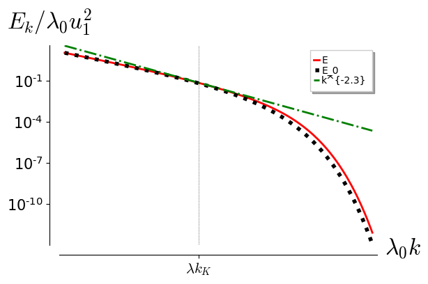
We plot a typical spectrum in fig. (2)
V Final remarks
Our goal in this paper is to develop a practical tool to explore problems that can be regarded as perturbations of homogeneous, isotropic turbulence in Newtonian incompressible fluids.
To achieve this goal we have deployed functional methods, such as the EA approach to the MSR formalism, to obtain formal expressions that display the parametric dependence of the correlation functions in full. These formal expressions can be used to construct perturbative series in terms of a suitable small parameter, the Weissenberg number in the case of viscoelastic flow, or the inverse speed of light for a relativistic fluid.
Of course, to obtain results which may be matched against numerical and experimental data requires computing the expansion coefficients to a high accuracy. Achieving this accuracy may be regarded as a unsolved problem in itself. We sidestep this issue by relying on our understanding of fully developed turbulence. Thus we replace the formal path integrals by simple ansätze known to work in Kolmogorov turbulence. We regard this procedure as an extreme, but valid, kind of renormalization [64].
As a final remark on this subject, we note that the application of field theory methods to turbulence is almost as old as the K41 theory itself [65, 66, 67, 68, 69, 70, 71, 72, 73, 74]. The MSR approach is typically seen as the most systematic way to translate a classical stochastic problem into a field theory. It has been used extensively in turbulence (to cite a few examples, see [75, 76, 77, 78, 79]). However, there remain lingering doubts on whether these methods can provide a convincing derivation of the K41 theory, let alone a means to improve it, such as providing a better prediction of the scaling exponents for the higher structure functions [28, 29, 30, 31, 32, 33]. Replacing the unknown correlations by their K41 form is a way to mimic the yet undiscovered non-perturbative methods necessary to compute them from first principles.
We would like to conclude with a few comments on our results.
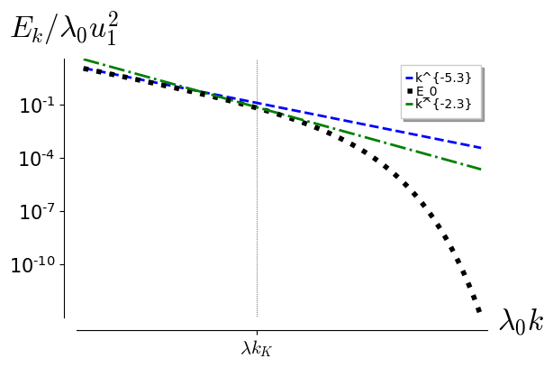
It is customary to fit turbulent spectra to power laws and in this sense a exponent for velocity correlations in Non Newtonian fluids has been reported, see eg. [8, 10]. This scaling does not seem to emerge from our analysis. However, as fig. (1) shows, for moderate Reynolds numbers the spectrum spans a range of scaling laws in the transition from the inertial to the dissipative range. For (as shown in fig. (1)) it actually displays a scaling around the Kolmogorov scale. The Non-Newtonian spectrum in fig. (2) shows a similar behavior.
This could be a case where two completely different analytic expressions nevertheless yield similar results. This is not uncommon, the agreement between the Colebrook formula and the Blasius law for the friction factor in pipe turbulence comes to mind [80].
A remarkable property of the spectrum eq. (56), clearly shown in fig. (2), is the enhancement of velocity fluctuations for very small scales, deep in the dissipative range, relative to the already strongly suppressed Newtonian spectrum of eq. (37). To the best of our understanding, this is not ruled out by available data, such as those in refs. ([6]), ([8]) and ([10]), but it may well be a make or break issue for the validation of the model.
Regarding this last point, we believe that the most relevant feature of our results is the way they display the functional dependence of the non-Newtonian spectrum on the different parameters of the theory. Validating this theoretical prediction requires comparing it against numerical and experimental data accross a full range of Reynolds and Weissenberg numbers.
We stress that we have discussed flows which are strictly homogeneous and isotropic. Data obtained from different configurations, such as wall-bounded flow ([8]), while relevant, cannot be directly compared to our theory.
In conclusion, our goal is to establish the cogency of our proposal, with its validation to be discussed in future communications.
Acknowledgements.
I thank P. Mininni for multiple talks. E. C. acknowledges financial support from Universidad de Buenos Aires through Grant No. UBACYT 20020170100129BA, CONICET Grant No. PIP2017/19:11220170100817CO and ANPCyT Grant No. PICT 2018: 03684.Appendix A Non-Newtonian fluid as the non-relativistic limit of a conformal fluid
We consider a relativistic fluid of massless particles.
At the macroscopic level, the theory is described by the energy-momentum tensor (EMT) . Adopting the Landau prescription for the four velocity and the energy density
| (64) |
and observing that is traceless, we are led to write
| (65) |
where
| (66) |
and
| (67) |
We must also provide an entropy flux. For an ideal fluid, namely when , the entropy density is
| (68) |
where is the temperature and is the pressure. From the thermodynamic relation
| (69) |
we conclude that
| (70) |
for some constant . The entropy flux is then
| (71) |
When we consider the real fluid, , we observe that because of (67) we cannot make a vector out of and . Therefore it makes sense to write
| (72) |
The entropy density ought to be maximum when the fluid is in equilibrium, namely when vanishes. So at least close to equilibrium we should have
| (73) |
for some dimensionless constant . If we further write
| (74) |
Then the conservation laws are
| (75) |
On the other part, positive entropy creation yields
| (76) |
which using the conservation laws and the transversality of may be written as
| (77) |
where
| (78) |
is the covariant form of the shear tensor eq. (3). Therefore, positive entropy creation is achieved by adopting the Cattaneo-Maxwell equation
| (79) |
We shall now consider the nonrelativistic limit. We write explicitly and
| (84) |
where . Observe that
| (85) |
The first nontrivial terms in the energy conservation equation are of order and read
| (86) |
From the momentum conservation equation we get
| (87) |
The Cattaneo-Maxwell equation (79) yields
| (88) |
A consistent nonrelativistic limit requires . Then from energy conservation we get to lowest order. Let us write
| (89) |
where .
Collecting again the leading terms we get
| (90) |
| (91) |
Taking the divergence of this equation we get
| (92) |
so we may write a scalar-free equation of motion
| (93) |
where
| (94) |
Finally
| (95) |
We may define a mass density
| (96) |
Then is constant to order . We see that , where is the non-constant part of the pressure. is not a dynamical variable but it is determined from the constraint
| (97) |
We see that we recover equations (1) in the particular case .
Appendix B Random Galilean invariance
Let us go back to the action functional eq. (4) and the corresponding generating functional eq. (5), whose Legendre transform yields the 1PI effective action , eq. (8).
This construction misses the fact that the equations of motion (1) are random galilean invariant, that is, they are invariant under the transformation
| (98) |
where is an arbitrary time dependent field. Of course we are using that
| (99) |
For this reason the path integral defining the generating functional, eq. (5), is redundant. To eliminate the overcounting, we consider the non-invariant function
| (100) |
Assuming that transforms as we see that
| (101) |
where is the total mass of the fluid. We now observe that
| (102) |
Introducing this identity into the path integral, we can take the integral out as a constant factor (for this we make a change of variables within the integral, with unit Jacobian), integrate over the with a Gaussian weight and exponentiate the determinant introducing Grassmann variables and , where now
| (103) |
where
| (104) |
Note that the ghost fields are decoupled. This action is still invariant under a BRST transformation defined as follows: the matter and auxiliary fields transform as in a random galilean transformation with parameter , where is a Grassmann constant, transforms into , and is invariant. We thus obtain the Zinn-Justin equation [81]
| (105) | |||||
Since the integral over ghost fields is just a decoupled Gaussian integral, the binary products decouple, namely
| (106) |
etc., and
| (107) |
Moreover
| (108) |
So eq. (105) is consistent with
| (109) |
where is independent of . is an effective action without the Fadeev-Popov procedure. This implies that is identically zero when the auxiliary fields vanish, independently of the physical fields.
In the presence of the gauge-fixing term and are unchanged, and now
| (110) |
When this forces the noise kernels and the self energies to vanish at zero momentum, as we have assumed in the text.
Appendix C Derivation of eq. (49)
We may estimate as follows. First note that at becomes a Lagrange multiplier enforcing the constraint
| (111) |
Now use a quasi-Gaussian approximation to get
| (113) | |||||
Since the integral is dominated by the infrared band, we approximate . Observe that two of the integrals vanish from symmetry, so
| (114) |
We filter out a longitudinal term and use again the spherical symmetry to get
| (115) |
is given in eq. (37). Since the integrals are cut off at , the first integral is the dominant one. We observe that the integral diverges as , keeping only the most divergent term we get
| (116) |
We finally approximate
Appendix D Computation of the Non-Newtonian spectrum
In this Appendix we give details of the derivation of eq. (56). We begin by writing from eq. (53) as
| (118) |
Both are real and positive; when , and ; this shows we are dealing with a singular limit.
The integral over in (56) is computed by contour methods and yields
| (120) |
To obtain eq. (56) we substitute these expressions and develop the result to first order in .
References
- [1] S. Chandrasekhar, The theory of turbulence, editado por E. Spiegel, Springer (2011).
- [2] A. S. Monin and A. M. Yaglom, Statistical Fluid Mechanics, MIT Press, 1971.
- [3] U. Frisch, Turbulence, the Legacy of A. N. Kolmogorov (Cambridge University Press, Cambridge, England, 1995).
- [4] J. L. Lumley, Turbulence in NonNewtonian Fluids, Physics of Fluids (1958-1988) 7, 335 (1964).
- [5] H. J. Seybold, H. A. Carmona, H. J. Herrmann and J. S. Andrade Jr., Self-organization and Nonuniversal Anomalous Scaling in Non-Newtonian Turbulence, Phys. Rev. Fluids 4, 064604 (2019).
- [6] Zhang, Y. B., Bodenschatz, E., Xu, H. and Xi, H. D. Experimental observation of the elastic range scaling in turbulent flow with polymer additives. Sci. Adv. 7, eabd3525 (2021).
- [7] Khalid M. Saqr and Iham F. Zidane, On non‑Kolmogorov turbulence in blood flow and its possible role in mechanobiological stimulation, Scientific Reports. 12, 13166 (2022).
- [8] Mitishita, R. S., MacKenzie, J. A., Elfring, G. J. and Frigaard, I. A. Fully turbulent flows of viscoplastic fluids in a rectangular duct. J. Non-Newtonian Fluid Mech. 293, 104570 (2021).
- [9] Rosti, M. E., Perlekar, P. and Mitra, D. Large is different: non-monotonic behaviour of elastic range scaling in polymeric turbulence at large Reynolds and Deborah numbers. Sci. Adv. 9, eadd3831 (2023).
- [10] Abdelgawad MS, Cannon I, Rosti ME. Scaling and intermittency in turbulent flows of elastoviscoplastic fluids. Nature Physics. 2023 Jul;19(7):1059-63.
- [11] R. K. Singh, P. Perlekar, D. Mitra and M. E. Rosti, Intermittency in the not-so-smooth elastic turbulence, Nature Communications 15:4070 ( 2024) (https://doi.org/10.1038/s41467-024-48460-5).
- [12] A. Chiarini, R. K. Singh and M. E. Rosti, Extending Kolmogorov Theory to Polymeric Turbulence, arXiv:2410.03237v2 (2024).
- [13] G. L. Eyink and Th. D. Drivas, Cascades and Dissipative Anomalies in Relativistic Fluid Turbulence, Phys. Rev. X 8, 011023 (2018).
- [14] Esteban Calzetta, Fully developed relativistic turbulence, Phys. Rev. D 103, 056018 (2021).
- [15] P.C. Martin, E.D. Siggia and H.A. Rose, Statistical Dynamics of Classical Systems, Phys. Rev. A8 423 (1973).
- [16] R Phythian, The functional formalism of classical statistical dynamics, J. Phys. A: Math. Gen., Vol. 10, No. 5, 777 (1977).
- [17] G.L. Eyink, Turbulence Noise, J. Stat. Phys. 83, 955 (1996).
- [18] A. Kamenev, Field Theory of Non-Equilibrium Systems, Cambridge University Press, Cambridge, U.K. (2011).
- [19] J. Zanella and E. Calzetta, Renormalization group and nonequilibrium action in stochastic field theory, Phys. Rev. E 66 036134 (2002).
- [20] C. de Dominicis and I. Giardina, Random fields and spin glasses: a field theory approach (Cambridge University Press, Cambridge, England, 2006).
- [21] J. Rammer, Quantum field theory of nonequilibrium states (Cambridge University Press, Cambridge (England), 2007)
- [22] E. Calzetta and B-L. Hu, Nonequilibrium Quantum Field Theory (Cambridge University Press, Cambridge, England, 2008).
- [23] P. Kovtun, Lectures on hydrodynamic fluctuations in relativistic theories, J. Phys. A 45, 473001 (2012).
- [24] P. Kovtun, G.D. Moore and P. Romatschke, Towards an effective action for relativistic dissipative hydrodynamics, JHEP 07, 123 (2014).
- [25] M. Harder, P. Kovtun and A. Ritz, On thermal fluctuations and the generating functional in relativistic hydrodynamics, JHEP 07, 025 (2015).
- [26] F. M. Haehl, R. Loganayagam and M. Rangamani, Effective action for relativistic hydrodynamics: fluctuations, dissipation, and entropy inflow, JHEP 10, 194 (2018).
- [27] N. Mirón Granese, A. Kandus and E. Calzetta, Field Theory Approaches to Relativistic Hydrodynamics. Entropy 24, 1790 (2022).
- [28] R. Kraichnan, An almost-Markovian Galilean-invariant turbulence model, J. Fluid Mech. 47, part 3, 513, (1971).
- [29] S Gauthier, M-E Brachet and J-D Fournier, Testing field-theoretical methods on a classical cubic equation with stochastic driving, J. Phys. A: Math. Gen. 14, 2969 (1981).
- [30] M. J. Giles, Is the renormalization group useless in turbulence?, Eur. J. Mech. B/Fluids, 17, no 4, 519 (1998).
- [31] A. Tsinober, An informal conceptual introduction to turbulence (Springer, Dordretch, 2009).
- [32] D. McComb, Jackson R. Herring and the Statistical Closure Problem of Turbulence: A Review of Renormalized Perturbation Theories, Atmosphere 14, 827 (2023).
- [33] D. McComb, What is isotropic turbulence and why is it important?, arXiv:2403.13962v1 (2024).
- [34] R. J. Gordon and W. R. Schowalter, Anisotropic Fluid Theory: A Different Approach to the Dumbbell Theory of Dilute Polymer Solutions, Trans. Soc. Rheol. 16, 79 (1972).
- [35] M. Doi and S. F. Edwards, The theory of polymer dynamics (Clarendon Press, Oxford, 1986).
- [36] Saramito, P. A new constitutive equation for elastoviscoplastic fluid flows. J. Non-Newtonian Fluid Mech. 145, 1–14 (2007).
- [37] Alexander Morozov and Saverio E. Spagnolie, Introduction to Complex Fluids, in S. Spagnolie (ed.), Complex Fluids in Biological Systems (Springer, New York, 2015).
- [38] J. L. Lumley, Drag reduction by additives, Ann. Rev. Fluid Mech. 1, 367 (1969).
- [39] P. S. Virk, Drag reduction fundamentals. AIChE J. 21, 625–656 (1975).
- [40] P. G. de Gennes, Introduction to polymer dynamics (Cambridge UP, Cambridge (England), 1990)
- [41] R. B. Bird, C. F. Curtiss, R. C. Armstrong and O. Hassager, Dynamics of Polymer Liquids, Vol 2, (John Wiley, New York, 1987).
- [42] E. Calzetta, Drag reduction by polymer additives from turbulent spectra, Phys. Rev. E 82, 066310 (2010).
- [43] E. Muratspahic, L. Brandfellner, J. Schöffmann, A. Bismarck, and H. W. Müller, Aqueous Solutions of Associating Poly(acrylamide-co-styrene): A Path to Improve Drag Reduction?, Macromolecules 55, 10479 (2022).
- [44] L. Rezzolla and O. Zanotti, Relativistic Hydrodynamics (Oxford University Press, Oxford, 2013).
- [45] P. Romatschke and U. Romatschke, Relativistic fluid dynamics in and out equilibrium - Ten years of progress in theory and numerical simulations of nuclear collisions (Cambridge University Press, Cambridge (England), 2019).
- [46] L. Cantarutti and E. Calzetta, Dissipative-type theories for Bjorken and Gubser flows, International Journal of Modern Physics A Vol. 35, 2050074 (2020).
- [47] H. Tennekes and J. L. Lumley, A first course in turbulence (MIT Press, Cambridge, 1972).
- [48] R. Kraichnan, Phys. Fluids 7, 1723 (1964) Kolmogorov’s hypotheses and eulerian turbulence theory
- [49] H. Horner and R. Lipowsky, On the Theory of Turbulence: A non Eulerian Renormalized Expansion, Z. Physik B 33, 223 (1979).
- [50] A. Berera, and D. Hochberg, Galilean invariance and homogeneous anisotropic randomly stirred flows, PHYSICAL REVIEW E 72, 057301 2005.
- [51] A. Berera and D. Hochberg, Gauge symmetry and Slavnov-Taylor identities for randomly stirred fluids, Phys. Rev. Lett. 99, 254501 (2007).
- [52] A. Berera, and D. Hochberg, Gauge fixing, BRS invariance and Ward identities for randomly stirred flows, Nuclear Physics B 814 [FS] (2009) 522–548.
- [53] S. A. Orszag, Analytical theories of turbulence, J. Fluid Mech. 41, part 2, 363 (1970).
- [54] W.D. McComb, The Physics of Fluid Turbulence (Clarendon Press, Oxford, 1994).
- [55] T. von Kármán, Progress in the statistical theory of turbulence. Proc. Natl. Acad. Sci. USA 34, 530 (1948).
- [56] R. H. Kraichnan, The structure of isotropic turbulence at very high Reynolds numbers, J. Fluid Mech. 5, 497 (1959).
- [57] J. O. Hinze, Turbulence (McGraw-Hill, New York, 1975).
- [58] S. B. Pope, Turbulent Flows (Cambridge University Press, Cambridge, England, 2000).
- [59] K. R. Sreenivasan, On the universality of the Kolmogorov constant, Phys. Fluids 7 (11), 2778 (1995).
- [60] I. Proudman and W. H. Reid, On the decay of a normally distributed and homogeneous turbulent velocity field, Philos. Trans. R. Soc. London, Ser. A 247, 163 (1954).
- [61] Henry Chang, Robert D. Moser, An inertial range model for the three-point third-order velocity correlation, Physics of Fluids 19, 105111 (2007).
- [62] A. V. Kopyev and K. P. Zybin, Exact result for mixed triple two-point correlations of velocity and velocity gradients in isotropic turbulence, Journal of Turbulence, DOI: 10.1080/14685248.2018.1511055 (2018).
- [63] E. A. Novikov, Functionals and the random-force method in turbulence theory, J. Exptl. Theoret. Phys. (U.S.S.R.) 47, 1919-1926 (Eng. trans. Sov. Phys. JETP 20, 1290 (1965).
- [64] W.D. McComb, Renormalization Methods (Clarendon Press, Oxford, 2004).
- [65] G. Eyink and U. Frisch, Robert H. Kraichnan, in P. Davidson et al. (editors)A Voyage through Turbulence (Cambridge U.P., Cambridge, 2011).
- [66] Wyld, H.W., Jr. Formulation of the Theory of Turbulence in an Incompressible Fluid. Ann. Phys. 1961, 14, 143–165.
- [67] L. L. Lee, A Formulation of the Theory of Isotropic Hydromagnetic Turbulence in an Incompressible Fluid, Ann. Phys. 32, 292 (1965).
- [68] V. I. Belinicher and V.S. L’vov, A scale-invariant theory of fully developed hydrodynamic turbulence, Zh. Eksp. Teor. fiz. 93, 533 (1987) (Engl. Trans. Sov. Phys. JETP 66, 303 (1987)).
- [69] V. S. L’vov, and I. Procaccia, Exact resummations in the theory of hydrodynamic turbulence II: A ladder to anomalous scaling, Phys. Rev. E52, 3858 (1996).
- [70] V. I. Belinicher, V. S. L’vov, and I. Procaccia, A new approach to computing the scaling exponents in fluid turbulence from first principles, Physica A 254, 215 (1998).
- [71] V. S. L’vov, and I. Procaccia, Computing the scaling exponents in fluid turbulence from first principles: the formal setup, Physica A 257, 165 (1998).
- [72] A.N.Vasil’ev, The Field Theoretic Renormalization Group in Critical Behavior Theory and Stochastic Dynamics (CRC, London, 1998).
- [73] A. Berera, M. Salewski and W. D. McComb, Eulerian field-theoretic closure formalisms for fluid turbulence, Phys. Rev. E 87, 013007 (2013).
- [74] L. Ts. Adzhemyan and Y. Kirienko, Theory of Turbulence for : Four-Loop Approximation of the Renormalization Group, arXiv:2406.14575 (2024).
- [75] V. I. Belinicher and V. S. L’vov, A scale-invariant theory of fully developed hydrodynamic turbulence, Zh. Eksp. Teor. Fiz. 93, 533 (1987) (Engl. trans. Sov. Phys. JETP 66, 303 (1987).
- [76] G. L. Eyink, Large-N limit of the “spherical model” of turbulence, Phys. Rev. E49, 3990 (1994).
- [77] W. D. Thacker, A path integral for turbulence in incompressible fluids, Journal of Mathematical Physics 38, 300 (1997).
- [78] P. Tomassini, An exact renormalization group analysis of 3D well developed turbulence, Physics Letters B 411, 117 (1997).
- [79] S. Flores and J-B. Fouvry, Vector Resonant Relaxation and Statistical Closure Theory. I. Direct Interaction Approximation, arXiv:2406.19306 (2024).
- [80] H. Schlichting, Boundary Layer Theory (McGraw-Hill, New York, 1979).
- [81] J. Zinn-Justin, Quantum Field Theory and Critical Phenomena (Clarendon Press, Oxforf, 1993).