On the Distribution of SINR for Cell-Free Massive MIMO Systems

During the uplink training phase, each user simultaneously transmits a pilot sequence to all APs, with the length of the pilot sequence denoted as $l_{p}$. Define $i_{k}\in\left\{1,\dots,l_{p}\right\}$ as the index of the pilot used by user $k$, represented by $\boldsymbol{\phi}_{i_{k}}\in\mathbb{C}^{l_{p}\times 1}$. We assume that $l_{p}\leq K$, which indicates that some users will share the same pilot sequence. Consequently, we define $\mathcal{P}_{k}\subset\mathcal{K}$ as the set of indices, including $k$, corresponding to users assigned the same pilot as user $k$. Therefore, for any user $k_{1}$ where $k_{1}\neq k$, the condition $i_{k}=i_{k_{1}}\Leftrightarrow k_{1}\in\mathcal{P}_{k}$ holds true. The pilot sequences are mutually orthogonal and the inner product of pilot sequences is given by

The pilot signal received by AP $m$, denoted as $\mathbf{Y}_{m}^{p}$, can be expressed as

where $\rho_{p}$ denotes the normalized pilot power, and $\mathbf{Z}_{m}^{p}\in\mathbb{C}^{N\times l_{p}}$ corresponds to the additive Gaussian noise matrix at AP $m$ during the uplink training phase, each element of which is independent and follows the distribution of $\mathcal{CN}(0,1)$.

To estimate the channel to user $k$, AP $m$ performs a correlation operation between the received pilot signal and the corresponding pilot sequence $\boldsymbol{\phi}_{i_{k}}$. Subsequently, it applies the MMSE technique to obtain the MMSE channel estimate $\hat{\mathbf{h}}_{mk}$ [12], which can be calculated as

where $\kappa_{mk}$ is defined as

The channel estimation follows the distribution of $\mathcal{CN}(0,c_{mk}\mathbf{I}_{N})$ with $c_{mk}$ given by [12]

Then, denote $\bar{\mathbf{h}}_{mk}=\mathbf{h}_{mk}-\hat{\mathbf{h}}_{mk}$ as the channel estimation error, which is independent of $\hat{\mathbf{h}}_{mk}$ and follows the distribution of $\mathcal{CN}(0,(\beta_{mk}-c_{mk})\mathbf{I}_{N})$. When multiple users share the same pilot sequence, their channel estimates are parallel to each other. This relationship can be expressed as

During downlink data training, all APs transmit signals to all users. The signal transmitted by AP $m$ is given by

where $\rho_{d}$ represents the normalized downlink transmission power each AP and $\eta_{mk}$ denotes power control coefficient from AP $m$ to user $k$. The symbol $q_{k}$, which satisfies $\mathbb{E}\left\{\left|q_{k}\right|^{2}\right\}=1$, is the symbol intended for the user $k$ during downlink data transmission and $\mathbf{b}_{mk}$ is precoding vector.

The precoding vector $\mathbf{b}_{mk}$ for user $k$ at AP $m$ is determined based on the channel estimation. The matrix of the channel estimates, $\hat{\mathbf{H}}_{m}=\left[\hat{\mathbf{h}}_{m1},\hat{\mathbf{h}}_{m2},\cdots,\hat{\mathbf{h}}_{mK}\right]\in\mathbb{C}^{N\times K}$, is rank-deficient due to the pilot sequence length being smaller than the number of users. To obtain a full-rank matrix of channel estimates, denoted as $\bar{\mathbf{H}}_{m}\in\mathbb{C}^{N\times l_{p}}$, we define $\bar{\mathbf{H}}_{m}=\mathbf{Y}_{m}^{p}\boldsymbol{\Phi}$, where $\boldsymbol{\Phi}=\left[\boldsymbol{\phi}_{1},\dots,\boldsymbol{\phi}_{l_{p}}\right]\in\mathbb{C}^{l_{p}\times l_{p}}$ is the pilot-book matrix [12]. The channel estimate between AP $m$ and user $k$ can be expressed in terms of $\bar{\mathbf{H}}_{m}$ as

where $\mathbf{e}_{k}$ represent the $i_{k}$th column of unit matrix $\mathbf{I}_{l_{p}}$. We consider using MRT and FZF precoding during downlink data transmission [11, 12], the precoding vector $\mathbf{b}_{mk}$ for user $k$ can be expressed as follows:

Each user receives the signals from all APs and the received signal at user $k$ is

where $z_{k}$ is the noise at user $k$ with the distribution of $\mathcal{CN}(0,1)$. Then, the SINR of user $k$ during downlink data transmission is given in (12).

In this subsection, we derive the distribution of SINR when MRT precoding is used. In the presence of multiple users receiving signals from all APs simultaneously, it becomes evident from equation (12) that all signals are interconnected, giving rise to the formation of the DS and the IN. Consequently, directly analyzing the distribution of SINR under MRT precoding is a challenging task. To overcome this difficulty, we adopt a feasible approach in the subsequent analysis. Firstly, we scrutinize the expressions for the distribution of DS and IN individually. Subsequently, by utilizing the derived expressions for the distributions of DS and IN, we are able to obtain the distribution of SINR.

When the number of APs $M$ and number of antennas at each AP $N$ are large enough, the distribution of $\sum_{m\in\mathcal{M}}\sqrt{\eta_{k}}\mathbf{b}_{mk}^{H}\hat{\mathbf{h}}_{mk}$ is approximated as a Gaussian distribution. Then we can approximate $U_{k}^{1}$ as a Gamma distribution in the following lemma.

Since $\text{DS}_{k}=\rho_{d}U_{k}^{1}$, we have $\mathbb{E}\left\{\text{DS}_{k}\right\}=\rho_{d}\mathbb{E}\left\{U_{k}^{1}\right\}$ and $\mathbb{E}\left\{\text{DS}_{k}^{2}\right\}=\rho_{d}\mathbb{E}\left\{\left(U_{k}^{1}\right)^{2}\right\}$. Then, $\text{DS}_{k}^{\text{MRT}}$ can be approximated as a Gamma distribution with shape parameter $j_{k1}$ and scale parameter $\rho_{d}\chi_{k1}$, i.e., $\text{DS}_{k}^{\text{MRT}}\sim\text{Gamma}(j_{k1},\rho_{d}\chi_{k1})$, where $\text{DS}_{k}^{\text{MRT}}$ represents the $\text{DS}_{k}$ with MRT precoding.

Then we turn to analyze the distribution of $\text{IN}_{k}^{\text{MRT}}$, where $\text{IN}_{k}^{\text{MRT}}$ represents the $\text{IN}_{k}$ with MRT precoding. Similarly, the distribution of $\text{IN}_{k}^{\text{MRT}}$ can be approximated as a Gamma distribution. In the following lemma, we approximate $\text{IN}_{k}^{\text{MRT}}$ as a Gamma distribution.

Based on the above analysis, we have obtained the distributions of the two components of the SINR: DS and IN. By leveraging the independence property between these two components, we can obtain the distribution of SINR in the CF mMIMO system which is shown in the following theorem.

Different from MRT precoding, FZF precoding can suppress inter-user interference. The FZF precoding vector used by AP $m$ towards user $k$ is given in (10), and the denominator of the precoding vector is given in closed form by [12]

where $(a)$ is obtained based on [33, Lemma 2.10], for a $l_{p}\times l_{p}$ central complex Wishart matrix with $M$ degrees of freedom satisfying $M\geq l_{p}+1$. Interference between users using different pilot sequences is suppressed and the product between $\hat{\mathbf{h}}_{mk}^{H}$ and $\mathbf{b}_{mk^{\prime}}$ can be calculated as follows [12]:

Then we can obtain the value of $\text{DS}_{k}$ based on (21) as follows:

where $\text{DS}_{k}^{\text{FZF}}$ represents the $\text{DS}_{k}$ with FZF precoding.

Similar to the analysis under MRT precoding, we approximate the distribution of $\text{IN}_{k}^{\text{FZF}}$ under FZF precoding as a Gamma distribution in the following lemma.

We calculate the value of $\text{DS}_{k}^{\text{FZF}}$ and obtain the distribution of $\text{IN}_{k}^{\text{FZF}}$ above. Then the distribution of SINR under the FZF precoding can be obtained as shown in the following theorem.

When MRT precoding is used in the CF mMIMO system, then the lower bound of achievable downlink rate is given in (33) [12]. The achievable rate in the CF mMIMO system with MRT precoding employed is given in the following lemma.

Consider the encoding rate of user $k$ is $r_{k}^{\text{MRT}}$ in the CF mMIMO system unser MRT precoding. An outage event for user $k$ when the SINR cant support the target rate $r_{k}^{\text{MRT}}$. The outage probability of user $k$ in the CF mMIMO system is given by

When FZF precoding is used in the CF mMIMO system, then the lower bound of achievable downlink rate is given (34) [12].

The achievable rate in the CF mMIMO system with FZF precoding employed is given in the following lemma.

Consider the encoding rate of user $k$ is $r_{k}^{\text{MRT}}$ in the CF mMIMO system under FZF precoding. The outage probability of user $k$ is given by

In our simulations, we consider a system of randomly distributed APs and users within a rectangular area measuring $1km\times 1km$. The large-scale fading coefficient, which accounts for both path loss and shadowing effects, is denoted as $\beta_{mn}=PL_{mn}+z_{mn}$, where $PL_{mn}$ represents the path loss component, while $z_{mn}\sim\mathcal{CN}(0,\delta_{sh}^{2})$ represents the shadowing component following a complex Gaussian distribution with a mean of zero and a variance of $\delta_{sh}^{2}$. To characterize the path loss, we employ a three-slope model proposed in [11] and adopt the same parameter settings as described in that paper. In addition, we set the pilot power to 20 dBm and the downlink transmit power to 23 dBm. The system bandwidth is 2 MHz and the power of Gaussian noise is -174 dB/Hz. The pilots are sequentially assigned to users, i.e., $i_{k}=\text{rem}\left(k,l_{p}\right)$, where $\text{rem}\left(,\right)$ represents the remainder operation. We employ the heuristic power allocation scheme introduced in [12], and the power allocation coefficients are computed using the following equation:

For the specific configuration details regarding the number of APs, users, the number of antennas per AP, and the pilot length in the system, we will provide them during the corresponding experiments.

Once MRT precoding is implemented in CF mMIMO systems, the CDF of DS and IN, concerning the variation in the number of antennas at the AP, are illustrated in Fig. 1 and Fig. 2, respectively. As anticipated, both DS and IN exhibit a corresponding increase with the augmentation of antenna quantity. This phenomenon can be attributed to the fact that a higher number of antennas enables the AP to transmit a greater number of signals, consequently leading to an enhancement in signal strength. Furthermore, the results derived from our theoretical analysis align closely with the outcomes obtained through Monte Carlo simulations. This congruence serves as evidence supporting the accuracy of our conclusions.

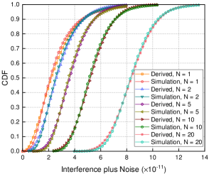
In Fig. 3, we investigate the impact of the variation in the number of antennas at each AP on the CDF of IN when FZF precoding is deployed. As the number of antennas increases at each AP, interference becomes more severe, resulting in a proportional increase of IN. Moreover, the graph illustrates a close alignment between the distribution derived from our theoretical analysis and the distribution obtained through Monte Carlo simulations, providing strong evidence that our conclusions are accurate.

We compare the CDF of the SINR for varying numbers of users under FZF precoding, as illustrated in Fig. 4. It is evident that as the number of users increases, the derived results closely converge with the Monte Carlo simulation results, eventually reaching a consistent agreement. This convergence is attributed to our approximation of the IN based on the CLT. As the number of users grows, this approximation becomes increasingly accurate and approaches the true results. Furthermore, with an increasing number of users, the SINR correspondingly decreases. Despite the unchanged length of the pilot sequence, more users share the same pilot, resulting in significant pilot contamination and subsequently causing severe interference, ultimately leading to a lower SINR.

In Fig. 5, we present the CDF of the SINR under the deployment of MRT precoding, showcasing its variation with respect to the number of users. As the number of users increases, the derived distribution of SINR exhibits a growing consistency with the results obtained from Monte Carlo simulations. This increasing alignment can be attributed to the heightened applicability of the CLT as the number of users expands. Furthermore, similar to the observation in the case of FZF precoding, the SINR decreases with an increasing number of users. The reason for this degradation in SINR is the same. Additionally, under MRT precoding, users who do not employ the same pilot sequence also introduce interference with each other. Consequently, employing FZF precoding in CF mMIMO systems generally yields higher SINR, indicating superior performance compared to MRT precoding.

We turn our attention to comparing the impact of varying the number of antennas on each AP under FZF precoding on the CDF of the SINR in CF mMIMO systems, as depicted in Fig. 6. It is evident that as the number of antennas increases, the derived results align more closely with the results obtained from system analysis. This convergence can be attributed to the increased number of constituent signals in the DS and IN due to the growing number of antennas, thereby enhancing the accuracy of the approximation based on the CLT. Furthermore, the increase in the number of antennas leads to an increase in SINR. From (22), it can be observed that DS increases with the growing number of antennas. While, according to (24), the $U_{kk_{1}}^{2}$ component of IN also increases with the number of users, (25) indicates that $U_{kk_{1}}^{3}$ remains unchanged with an increasing number of antennas. Hence, an increase in the number of antennas results in an improvement in SINR.

Fig. 7 illustrates the distribution of SINR under MRT precoding for different numbers of antennas. Similar to the scenario with FZF precoding, it is observed that as the number of antennas increases, the derived CDF of SINR closely aligns with the results obtained from Monte Carlo simulations. Furthermore, an increase in the number of antennas leads to an improvement in SINR. As MRT precoding only mitigates the influence of noise, while FZF precoding suppresses the effects of interference, FZF precoding generally achieves better performance.

We have investigated the impact of varying the number of antennas on each AP and the number of users on achievable rates under both FZF precoding and MRT precoding, as depicted in Fig. 8 and Fig. 9, respectively. It can be observed that the results derived from our analysis align with the results obtained from Monte Carlo simulations. As the number of users decreases and the number of antennas increases, the achievable rates also increase. This is because the reduction in the number of users and the increase in the number of antennas result in higher SINR, thereby leading to an increase in achievable rates. Besides, it can be observed that our derived results are higher than the lower bound with different scenarios. Under MRT precoding, our derived results are significantly higher than the lower bound. However, under FZF precoding, our derived results are only slightly higher than the lower bound. This is because, with FZF precoding, both desired signals and interference can be directly computed, and the uncertainty in SINR mainly comes from channel estimation errors. Therefore, compared to MRT precoding, FZF precoding yields a more stable SINR, resulting in actual achievable rates that are closer to the lower bound.

We conducted separate investigations on the impact of different coding rates and the number of antennas on each AP for outage probability under FZF precoding and MRT precoding, as depicted in Fig. 10 and Fig. 11, respectively. As anticipated, the outage probability increases continuously with higher coding rates and a reduced number of antennas on the APs. Moreover, it is noteworthy that our derived results closely align with the results obtained from Monte Carlo simulations across various scenarios.

References

- [1] K. Zheng, L. Zhao, J. Mei, B. Shao, W. Xiang, and L. Hanzo, “Survey of large-scale MIMO systems,” IEEE Commun. Surveys Tuts., vol. 17, no. 3, pp. 1738–1760, 3rd Quart., 2015.
- [2] H. Pei, X. Chen, X. Huang, X. Liu, X. Zhang, and Y. Huang, “Key issues and algorithms of multiple-input-multiple-output over-the-air testing in the multi-probe anechoic chamber setup,” Sci. China Inf. Sci., vol. 65, no. 3, p. 131302, 2022.
- [3] R. Feng, C.-X. Wang, J. Huang, and X. Gao, “Recent advances of ultramassive multiple-input, multiple-output technologies: Realizing a sixth-generation future in spatial and beam domains,” IEEE Veh. Technol. Mag., vol. 18, no. 1, pp. 70–79, Mar. 2023.
- [4] S. Elhoushy, M. Ibrahim, and W. Hamouda, “Cell-free massive MIMO: A survey,” IEEE Commun. Surveys Tuts., vol. 24, no. 1, pp. 492–523, 1st Quart., 2022.
- [5] A. Lozano, R. W. Heath, and J. G. Andrews, “Fundamental limits of cooperation,” IEEE Trans. Inf. Theory, vol. 59, no. 9, pp. 5213–5226, Sep. 2013.
- [6] F. Guo, H. Lu, and Z. Gu, “Joint power and user grouping optimization in cell-free massive MIMO systems,” IEEE Trans. Wireless Commun., vol. 21, no. 2, pp. 991–1006, Feb. 2022.
- [7] J. Zhang, S. Chen, Y. Lin, J. Zheng, B. Ai, and L. Hanzo, “Cell-free massive MIMO: A new next-generation paradigm,” IEEE Access, vol. 7, pp. 99 878–99 888, Jul. 2019.
- [8] Z. Chen and E. Björnson, “Channel hardening and favorable propagation in cell-free massive MIMO with stochastic geometry,” IEEE Trans. Commun., vol. 66, no. 11, pp. 5205–5219, Nov. 2018.
- [9] E. Nayebi, A. Ashikhmin, T. L. Marzetta, H. Yang, and B. D. Rao, “Precoding and power optimization in cell-free massive MIMO systems,” IEEE Trans. Wireless Commun., vol. 16, no. 7, pp. 4445–4459, Jul. 2017.
- [10] H. Q. Ngo, L.-N. Tran, T. Q. Duong, M. Matthaiou, and E. G. Larsson, “On the total energy efficiency of cell-free massive MIMO,” IEEE Trans. Green Commun. Netw., vol. 2, no. 1, pp. 25–39, Mar. 2018.
- [11] H. Q. Ngo, A. Ashikhmin, H. Yang, E. G. Larsson, and T. L. Marzetta, “Cell-free massive MIMO versus small cells,” IEEE Trans. Wireless Commun., vol. 16, no. 3, pp. 1834–1850, Mar. 2017.
- [12] G. Interdonato, M. Karlsson, E. Björnson, and E. G. Larsson, “Local partial zero-forcing precoding for cell-free massive MIMO,” IEEE Trans. Wireless Commun., vol. 19, no. 7, pp. 4758–4774, Jul. 2020.
- [13] J. Zhang, J. Zhang, E. Björnson, and B. Ai, “Local partial zero-forcing combining for cell-free massive MIMO systems,” IEEE Trans. Commun., vol. 69, no. 12, pp. 8459–8473, Dec. 2021.
- [14] E. Nayebi, A. Ashikhmin, T. L. Marzetta, and B. D. Rao, “Performance of cell-free massive MIMO systems with MMSE and LSFD receivers,” in Proc. 50th Asilomar Conf. Signals, Syst. Comput., Nov. 2016, pp. 203–207.
- [15] Z. Wang, J. Zhang, B. Ai, C. Yuen, and M. Debbah, “Uplink performance of cell-free massive MIMO with multi-antenna users over jointly-correlated rayleigh fading channels,” IEEE Trans. Wireless Commun., vol. 21, no. 9, pp. 7391–7406, Sep. 2022.
- [16] J. Zheng, J. Zhang, J. Cheng, V. C. M. Leung, D. W. K. Ng, and B. Ai, “Asynchronous cell-free massive MIMO with rate-splitting,” IEEE J. Sel. Areas Commun., vol. 41, no. 5, pp. 1366–1382, May. 2023.
- [17] A. Papazafeiropoulos, P. Kourtessis, M. D. Renzo, S. Chatzinotas, and J. M. Senior, “Performance analysis of cell-free massive MIMO systems: A stochastic geometry approach,” IEEE Trans. Veh. Commun., vol. 69, no. 4, pp. 3523–3537, Apr. 2020.
- [18] O. Özdogan, E. Björnson, and J. Zhang, “Performance of cell-free massive MIMO with rician fading and phase shifts,” IEEE Trans. Wireless Commun., vol. 18, no. 11, pp. 5299–5315, Nov. 2019.
- [19] Y. Fang, L. Qiu, X. Liang, and C. Ren, “Cell-free massive MIMO systems with oscillator phase noise: Performance analysis and power control,” IEEE Trans. Veh. Commun., vol. 70, no. 10, pp. 10 048–10 064, Oct. 2021.
- [20] H. Masoumi and M. J. Emadi, “Performance analysis of cell-free massive MIMO system with limited fronthaul capacity and hardware impairments,” IEEE Trans. Wireless Commun., vol. 19, no. 2, pp. 1038–1053, Feb. 2020.
- [21] Y. Zhang, M. Zhou, X. Qiao, H. Cao, and L. Yang, “On the performance of cell-free massive MIMO with low-resolution ADCs,” IEEE Access, vol. 7, pp. 117 968–117 977, Aug. 2019.
- [22] B. Al-Nahhas, M. Obeed, A. Chaaban, and M. J. Hossain, “Ris-aided cell-free massive MIMO: Performance analysis and competitiveness,” in Proc. IEEE Int. Conf. Commun. Workshops (ICC Workshops), Jun. 2021, pp. 1–6.
- [23] S. Kusaladharma, W.-P. Zhu, W. Ajib, and G. A. A. Baduge, “Stochastic geometry based performance characterization of swipt in cell-free massive MIMO,” IEEE Trans. Veh. Commun., vol. 69, no. 11, pp. 13 357–13 370, Nov. 2020.
- [24] Y. Li and G. A. Aruma Baduge, “NOMA-aided cell-free massive MIMO systems,” IEEE Wireless Commun. Lett., vol. 7, no. 6, pp. 950–953, Dec. 2018.
- [25] A. Mishra, Y. Mao, L. Sanguinetti, and B. Clerckx, “Rate-splitting assisted massive machine-type communications in cell-free massive MIMO,” IEEE Commun. Lett., vol. 26, no. 6, pp. 1358–1362, Jun. 2022.
- [26] P. Li, D. Paul, R. Narasimhan, and J. Cioffi, “On the distribution of SINR for the MMSE MIMO receiver and performance analysis,” IEEE Trans. Inf. Theory, vol. 52, no. 1, pp. 271–286, Jan. 2006.
- [27] H. Lim and D. Yoon, “On the Distribution of SINR for MMSE MIMO Systems,” IEEE Trans. Commun., vol. 67, no. 6, pp. 4035–4046, Jun. 2019.
- [28] H. Q. Ngo, E. G. Larsson, and T. L. Marzetta, “Energy and spectral efficiency of very large multiuser MIMO systems,” IEEE Trans. Commun., vol. 61, no. 4, pp. 1436–1449, Apr. 2013.
- [29] Y. Jiang, M. K. Varanasi, and J. Li, “Performance analysis of ZF and MMSE equalizers for MIMO systems: An in-depth study of the high snr regime,” IEEE Trans. Inf. Theory, vol. 57, no. 4, pp. 2008–2026, Apr. 2011.
- [30] Z. Zhang, X. You, D. Wang, X. Xia, P. Zhu, Y. Jiang, C. Liang, and J. Wang, “Performance of multidevice downlink cell-free system under finite blocklength for uRLLC with hard deadlines,” IEEE J. Sel. Areas Commun., pp. 1–1, 2023.
- [31] X. Zhang, J. Wang, and H. V. Poor, “Statistical delay and error-rate bounded qos provisioning for mURLLC over 6g cf M-MIMO mobile networks in the finite blocklength regime,” IEEE J. Sel. Areas Commun., vol. 39, no. 3, pp. 652–667, Mar. 2021.
- [32] Wolfram. Hypergeometric function. [Online]. Available: {https://reference.wolfram.com/language/ref/Hypergeometric2F1.html}
- [33] A. Edelman and N. R. Rao, “Random matrix theory,” Acta Numer., vol. 14, p. 233–297, 2005.
- [34] Wolfram. Generalized hypergeometric function. [Online]. Available: {https://reference.wolfram.com/language/ref/HypergeometricPFQ.html}