On the Convergence of SGD with Biased Gradients
Abstract
We analyze the complexity of biased stochastic gradient methods (SGD), where individual updates are corrupted by deterministic, i.e. biased error terms. We derive convergence results for smooth (non-convex) functions and give improved rates under the Polyak-Łojasiewicz condition. We quantify how the magnitude of the bias impacts the attainable accuracy and the convergence rates (sometimes leading to divergence).
Our framework covers many applications where either only biased gradient updates are available, or preferred, over unbiased ones for performance reasons. For instance, in the domain of distributed learning, biased gradient compression techniques such as top- compression have been proposed as a tool to alleviate the communication bottleneck and in derivative-free optimization, only biased gradient estimators can be queried. We discuss a few guiding examples that show the broad applicability of our analysis.
1 Introduction
The stochastic gradient descent (SGD) algorithm has proven to be effective for many machine learning applications. This first-order method has been intensively studied in theory and practice in recent years (cf. Bottou et al., 2018). Whilst vanilla SGD crucially depends on unbiased gradient oracles, variations with biased gradient updates have been considered in a few application domains recently.
For instance, in the context of distributed parallel optimization where the data is split among several compute nodes, the standard mini-batch SGD updates can yield a bottleneck in large-scale systems and techniques such as structured sparsity (Alistarh et al., 2018; Wangni et al., 2018; Stich et al., 2018) or asynchronous updates (Niu et al., 2011; Li et al., 2014) have been proposed to reduce communication costs. However, sparsified or delayed SGD updates are no longer unbiased and the methods become more difficult to analyze (Stich and Karimireddy, 2019; Beznosikov et al., 2020).
Another class of methods that do not have access to unbiased gradients are zeroth-order methods which find application for optimization of black-box functions (Nesterov and Spokoiny, 2017), or for instance in deep learning for finding adversarial examples (Moosavi-Dezfooli et al., 2016; Chen et al., 2017). Some theoretical works that analyze zeroth-order training methods argue that the standard methods often operate with a biased estimator of the true gradient (Nesterov and Spokoiny, 2017; Liu et al., 2018), in contrast to SGD that relies on unbiased oracles.
Approximate gradients naturally also appear in many other applications, such as in the context of smoothing techniques, proximal updates or preconditioning (d’Aspremont, 2008; Schmidt et al., 2011; Devolder et al., 2014; Tappenden et al., 2016; Karimireddy et al., 2018).
Many standard textbook analyses for SGD typically require unbiased gradient information to prove convergence (Lacoste-Julien et al., 2012; Bottou et al., 2018). Yet, the manifold applications mentioned above, witness that SGD can converge even when it has only access to inexact or biased gradient oracles. However, all these methods and works required different analyses which had to be developed separately for every application. In this work, we reconcile insights that have been accumulated previously, explicitly or implicitly, and develop novel results, resulting in a clean framework for the analysis of a general class of biased SGD methods.
We study SGD under a biased gradient oracle model. We go beyond the standard modeling assumptions that require unbiased gradient oracles with bounded noise (Bottou et al., 2018), but allow gradient estimators to be biased, for covering the important applications mentioned above. We find that SGD with biased updates can converge to the same accuracy as SGD with unbiased oracles when the bias is not larger than the norm of the expected gradient. Such a multiplicative bound on the bias does for instance hold for quantized gradient methods (Alistarh et al., 2017). Without such a relative bound on the bias, biased SGD in general only converges towards a neighborhood of the solution, where the size of the neighborhood depends on the magnitude of the bias.
Although it is a widespread view in parts of the literature that SGD does only converge with unbiased oracles, our findings shows that SGD does not need unbiased gradient estimates to converge.
Algorithm and Setting.
Specifically, we consider unconstrained optimization problems of the form:
| (1) |
where is a smooth function and where we assume that we only have access to biased and noisy gradient estimator. We analyze the convergence of (stochastic) gradient descent:
| (2) |
where is a sequence of step sizes and is a (potentially biased) gradient oracle for zero-mean noise , , and bias terms. In the case , the gradient oracle becomes unbiased and we recover the setting of SGD. If in addition almost surely, we get back to the classic Gradient Descent (GD) algorithm.
Contributions.
We show that biased SGD methods can in general only converge to a neighborhood of the solution but indicate also interesting special cases where the optimum still can be reached. Our framework covers smooth optimization problems (general non-convex problems and non-convex problems under the Polyak-Łojasiewicz condition) and unifies the rates for both deterministic and stochastic optimization scenarios. We discuss a host of examples that are covered by our analysis (for instance top- compression, random-smoothing) and compare the convergence rates to prior work.
2 Related work
Optimization methods with deterministic errors have been previously studied mainly in the context of deterministic gradient methods. For instance, Bertsekas (2002) analyzes gradient descent under the same assumptions on the errors as we consider here, however does not provide concise rates. Similar, but slightly different, assumptions have been made in (Hu et al., 2020a) that considers finite-sum objectives.
Most analyses of biased gradient methods have been carried out with specific applications in mind. For instance, computation of approximate (i.e. corrupted) gradient updates is for many applications computationally more efficient than computing exact gradients, and therefore there was a natural interest in such methods (Schmidt et al., 2011; Tappenden et al., 2016; Karimireddy et al., 2018). d’Aspremont (2008); Baes (2009); Devolder et al. (2014) specifically also consider the impact of approximate updates on accelerated gradient methods and show these schemes have to suffer from error accumulation, whilst non-accelerated methods often still converge under mild assumptions. Devolder et al. (2014); Devolder (2011) consider a notion of inexact gradient oracles that generalizes the notion of inexact subgradient oracles (Polyak, 1987). We will show later that their notion of inexact oracles is stronger than the oracles that we consider in this work.
In distributed learning, both unbiased (Alistarh et al., 2017; Zhang et al., 2017) and biased (Dryden et al., 2016; Aji and Heafield, 2017; Alistarh et al., 2018) compression techniques have been introduced to address the scalability issues and communication bottlenecks. Alistarh et al. (2018) analyze the top- compression operator which sparsifies the gradient updates by only applying the top components. They prove a sublinear rate that suffers a slowdown compared to vanilla SGD (this gap could be closed with additional assumptions). Biased updates that are corrected with error-feedback (Stich et al., 2018; Stich and Karimireddy, 2019) do not suffer from such a slowdown. However, these methods are not the focus of this paper. In recent work, Beznosikov et al. (2020) analyze top- compression for deterministic gradient descent, often denoted as greedy coordinate descent (Nutini et al., 2015; Karimireddy et al., 2019). We recover greedy coordinate descent convergence rates as a special case (though, we are not considering coordinate-wise Lipschitzness as in those specialized works). Asynchronous gradient methods have sometimes been studied trough the lens of viewing updates as biased gradients (Li et al., 2014), but the additional structure of delayed gradients admits more fine-grained analyses (Niu et al., 2011; Mania et al., 2017).
Another interesting class of biased stochastic methods has been studied in (Nesterov and Spokoiny, 2017) in the context of gradient-free optimization. They show that the finite-difference gradient estimator that evaluates the function values (but not the gradients) at two nearby points, provides a biased gradient estimator. As a key observation, they can show randomized smoothing estimates an unbiased gradient of a different smooth function that is close to the original function. This observation is leveraged in the proofs. In this work, we consider general bias terms (without inherent structure to be exploited), and hence our convergence rates are slightly weaker for this special case. Randomized smoothing was further studied in (Duchi et al., 2012; Bach and Perchet, 2016).
Hu et al. (2016) study bandit convex optimization with biased noisy gradient oracles. They assume that the bias can be bounded by an absolute constant. Our notion is more general and covers uniformly bounded bias as a special case. Other classes of biased oracle have been studied for instance by Hu et al. (2020b) who consider conditional stochastic optimization, Chen and Luss (2018) who consider consistent biased estimators and Wang and Giannakis (2020) who study the statistical efficiency of Q-learning algorithms by deriving finite-time convergence guarantees for a specific class of biased stochastic approximation scenarios.
3 Formal setting and assumptions
In this section we discuss our main setting and assumptions. All our results depend on the standard smoothness assumption, and some in addition on the PL condition.
3.1 Regularity Assumptions
Assumption 1 (-smoothness).
The function is differentiable and there exists a constant such that for all :
| (3) |
Sometimes we will assume the Polyak- Łojasiewicz (PL) condition (which is implied by standard -strong convexity, but is much weaker in general):
Assumption 2 (-PL).
The function is differentiable and there exists a constant such that
| (4) |
3.2 Biased Gradient Estimators
Finally, whilst the above assumptions are standard, we now introduce biased gradient oracles.
Definition 1 (Biased Gradient Oracle).
A map s.t.
for a bias and zero-mean noise , that is , .
We assume that the noise and bias terms are bounded:
Assumption 3 (-bounded noise).
There exists constants such that
Assumption 4 (-bounded bias).
There exists constants , and such that
Our assumption on the noise is similar as in (Bottou, 2010; Stich, 2019) and generalizes the standard bounded noise assumption (for which only is admitted). By allowing the noise to grow with the gradient norm and bias, an admissible parameter can often be chosen to be much smaller than under the constraint .
Our assumption on the bias is similar as in (Bertsekas, 2002). For the special case when one might expect (and we prove later) that gradient methods can still converge for any bias strength , as in expectation the corrupted gradients are still aligned with the true gradient, (see e.g. Bertsekas, 2002). In the case , gradient based methods can only converge to a region where . We make these claims precise in Section 4 below.
A slightly different condition than Assumption 4 was considered in (Hu et al., 2020a), but they measure the relative error with respect to the stochastic gradient , and not with respect to as we consider here. Whilst we show that biased gradient methods converge for any , for instance Hu et al. (2020a) required a stronger condition on -strongly convex functions (see also Remark 7 below).
4 Biased SGD Framework
In this section we study the convergence of stochastic gradient descent (SGD) with biased gradient oracles as introduced in Definition 1, see also Algorithm 1. For simplicity, we will assume constant stepsize , , in this section.
4.1 Modified Descent Lemma
A key step in our proof is to derive a modified version of the descent lemma for smooth functions (cf. Nesterov, 2004). We give all missing proofs in the appendix.
Lemma 2.
When we recover (even with the same constants) the standard descent lemma.
4.2 Gradient Norm Convergence
We first show that Lemma 2 allows to derive convergence on all smooth (including non-convex) functions, but only with respect to gradient norm, as mentioned in Section 3.2 above. By rearranging (5) and the notation , we obtain
and by summing and averaging over ,
where . We summarize this observation in the next lemma:
Lemma 3.
The quantity on the left hand side is equal to the expected gradient norm of a uniformly at random selected iterate, for and a standard convergence measure. Alternatively one could consider .
If there is no additive bias, , then Lemma 3 can be used to show convergence of SGD by carefully choosing the stepsize to minimize the term in the round bracket. However, with a bias SGD can only converge to a neighborhood of the solution.
Theorem 4.
If there is no bias, , then this result recovers the standard convergence rate of gradient descent (when also ) or stochastic gradient descent, in general. When the biased gradients are correlated with the gradient (i.e. , ), then the exact solution can still be found, though the number of iterations increases by a factor of in the deterministic case, or by if the noise term is dominating the rate. When there is an uncorrelated bias, , then SGD can only converge to a neighborhood of a stationary point and a finite number of iterations suffice to converge. This result is tight in general, as we show in Remark 5 below.
Remark 5 (Tightness of Error-floor).
Consider a -smooth function with gradient oracle , for , with and . This oracle has -bounded bias. For any stationary point with , it holds , i.e. .
4.3 Convergence under PL condition
To show convergence under the PL condition, we observe that (5) and (4) imply
| (6) |
By now unrolling this recursion we obtain the next theorem.
Theorem 6.
This result shows, that SGD with constant stepsize converges up to the error floor , given in (7). The second term in this bound can be decreased by choosing the stepsize small, however, the first term remains constant, regardless of the choice of the stepsize. We will investigate this error floor later in the experiments.
Without bias terms, we recover the best known rates under the PL condition (Karimi et al., 2016). Compared to the SGD convergence rate for -strongly convex function our bound is worse by a factor of compared to (Stich, 2019), but we consider convergence of the function value of the last iterate here.
Remark 7 (Convergence on Strongly Convex Functions.).
Theorem 6 applies also to -strongly convex functions (which are -PŁ) and shows convergence in function value for any (if ). By -strong convexity this implies iterate convergence , however, at the expense of an additional factor. For proving a stronger result, for instance to prove a one-step progress bound for (as it standard in the unbiased case (Lacoste-Julien et al., 2012; Stich, 2019)) it is necessary to impose a strong condition , similar as in (Hu et al., 2020a).
4.4 Divergence on Convex Functions
Albeit Theorem 4 shows convergence of the gradient norms, this convergence does not imply convergence in function value in general (unless the gradient norm is related to the function values, as for instance guaranteed by (4)). We now give an example of a weakly-convex (non-strongly convex) smooth function, where Algorithm 1 can diverge.
Example 8.
Consider the Huber-loss function ,
and define the gradient oracle . This is a biased oracle with , and it is easy to observe that iterations (2) diverge for any stepsize , given .
This result shows that in general it is not possible to converge when , and that the approximate solutions found by SGD with unbiased gradients (in Example 8 converging to 0) and by SGD with biased gradients can be arbitrarily far away. It is an interesting open question, whether SGD can be made robust to biased updates, i.e. preventing this diverging behaviour through modified updates (or stronger assumptions on the bias). We leave this for future work.
5 Discussion of Examples
In this section we are going to look into some examples which can be considered as special cases of our biased gradient framework. Table 1 shows a summary of these examples together with value of the respective parameters.
| def | M | 1-m | |||
|---|---|---|---|---|---|
| top- compression | 0 | ||||
| random- compression | 0 | 0 | |||
| random- compression (of stochastic g.) | 0 | ||||
| Gaussian smoothing | 4(d+4) | 1 | |||
| -oracle | (see text) | 0 | 0 | 1 | |
| stochastic -oracle | (see appendix) | 0 | 1 | ||
| compressed gradient | 0 | 0 | 0 |
5.1 Top- and Random- sparsification
The well-known top- spasification operator (Dryden et al., 2016; Alistarh et al., 2018) that selects the largest coordinates of the gradient vector is a biased gradient oracle with and . This means, that GD with top- compression converges to a stationary point on smooth functions and under the PL condition the convergence rate is when there is no additional noise. This recovers the rate of greedy coordinate descent when analyzed in the Euclidean norm (Nutini et al., 2015).
The biased random- sparsification operator randomly selects out of the coordinates of the stochastic gradient, and sets the other entries to zero. As , this implies a slowdown over the corresponding rates of GD (recovering the rate of random coordinate descent (Nesterov and Spokoiny, 2017; Richtárik and Takác, 2016)) and SGD, with asymptotic dominant term that is expected (cf. Chaturapruek et al., 2015). In the appendix we further discuss differences to unbiased random- sparsification.111By rescaling the obtained sparse vector by the factor one obtains a unbiased estimator (with higher variance). With these sparsification operators the dominant term in the rate remains , but the optimization terms can be improved as a benefit of choosing larger stepsizes. However, this observation does not show a limitation of the biased rand- oracle, but is merely a consequence of applying our general result to this special case. Both algorithms are equivalent when properly tuning the stepsize.
5.2 Zeroth-Order Gradient
Next, we discuss the zeroth-order gradient oracle obtained by Gaussian smoothing (cf. Nesterov and Spokoiny, 2017). This oracle is defined as (Polyak, 1987):
| (8) |
where is a smoothing parameter and a random Gaussian vector. Nesterov and Spokoiny (2017, Lemma 3 & Theorem 4) provide estimates for the bias:
and the second moment:
We conclude that Assumptions 3, and 4 hold with:
Nesterov and Spokoiny (2017) show that on smooth functions gradient-free oracles in general slow-down the rates by a factor of , similar as we observe here with . However, their oracle is stronger, for instance they can show convergence (up to ) on weakly-convex functions, which is not possible with our more general oracle (see Example 8).
5.3 Inexact gradient oracles
Devolder et al. (2014) introduced the notion of inexact gradient oracles. A -gradient oracle for is a pair that satisfies :
We have by (Devolder et al., 2014):
hence we can conclude: and .
It is important to observe that the notion of a oracle is stronger than what we consider in Assumption 4. For this, consider again the Huber-loss from Example 8 and a gradient estimator . For , we observe that it must hold , otherwise the condition of the oracle is violated. In contrast, the bias term in Assumption 4 can be constant, regardless of . Devolder (2011, preprint) generalized the notion of oracles to the stochastic case, which we discuss in the appendix.
5.4 Biased compression operators
The notion of top- compressors has been generalized to arbitrary -compressors, defined as
Definition 2 (-compressor).
if s.t.:
5.5 Delayed Gradients
Another example of updates that can be viewed as biased gradients, are delayed gradients, for instance arising in asynchronous implementations of SGD (Niu et al., 2011). For instance Li et al. (2014, Proof of Theorem 2) provide a bound on the bias. See also (Stich and Karimireddy, 2019) for a more refined analysis in the stochastic case. However, these bounds are not of the form as in Assumption 4, as they depend on past gradients, and not only the current gradient at . We leave generalizations of Assumption 4 for future work (moreover, delayed gradient methods have been analyzed tightly with other tools already).
6 Experiments
In this section we verify numerically whether our theoretical bounds are aligned with the numerical performance of SGD with biased gradient estimators. In particular, we study whether the predicted error floor (7) of the form can be observed in practice.
Synthetic Problem Instance.
We consider a simple least squares objective function , in dimension , where the matrix is chosen according to the Nesterov worst function (Nesterov, 2004). We choose this function since its Hessian, i.e., has a very large condition number and hence it is a hard function to optimize. By the choice of this objective function is strongly convex. We control the stochastic noise by adding Gaussian noise to every gradient.
6.1 Experiment with a synthetic additive bias
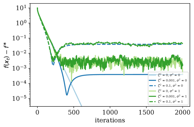
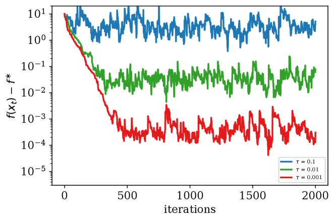
In our first setup (Figure 1), we consider a synthetic case in which we add a constant value to the gradient to control the bias, and vary the noise . This corresponds to the setting where we have , , .
Discussion of Results. Figure 1 highlights the effect of the parameters and on the rate of the convergence and the neighbourhood of the convergence. Notice that a small bias value can only affect the convergence neighborhood when there is no stochastic noise. In fact this matches the error floor we derived in (7). When is small compared to , i.e, the bias is insignificant compared to the noise, the second term in (7) determines the neighborhood of the optimal solution to which SGD with constant stepsize converges. In contrast, when is large the first term in (7) dominates the second term and determines the neighborhood of the convergence. As mentioned earlier in Section 4.3, the second term in (7) also depends on the stepsize, meaning that by increasing (decreasing) the stepsize the effect of in determining the convergence neighborhood can be increased (decreased).
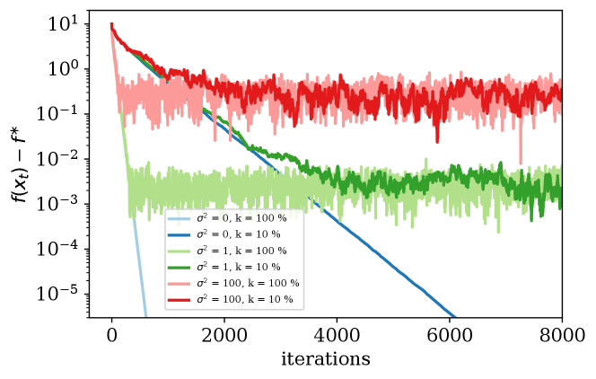
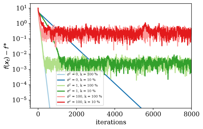
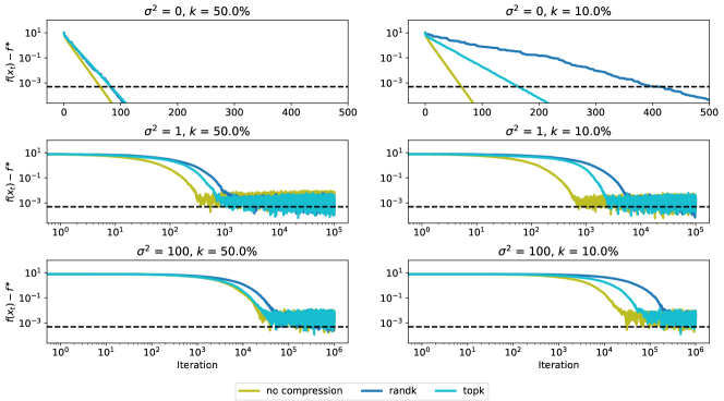
6.2 Experiment with Top- and Random- sparsification
In contrast to the previous section, we leave the completely synthetic setup, and consider structured bias that arises from compressing the gradients by using either the random- or top- method (Alistarh et al., 2018), displayed in Figures 2, 3. We use the same objective function as introduced earlier. In each iteration we compress the stochastic gradient, , by the top- or random- method, i.e.,
where is either or operator, for . As we showed in Section 5, this corresponds to the setting for rand-, and for top-, with .
Error floor. Figure 2, 3 show the effect of the parameters and (that determine the level of noise and bias respectively) on the rate of convergence as well as the error floor, when using random- and top- compressors and a constant stepsize .
Convergence rate. In Figure 5 we show the convergence for different noise levels and compression parameters . For each configuration and algorithm, we tuned the stepsize to reach the target accuracy (set by ) in the fewest number of iterations as possible.
Discussion of Results.
We can see that in this case even in the presence of stochastic noise, random- and top-, although with a slower rate, can still converge to the same level as with no compression. We note that top- consistently converges faster than rand-, for the same values of . The error floor for both schemes is mainly determined by the strength of the noise that dominates in (7). In Figure 5 we see that top- and random- can still converge to the same error level as no compression scheme but with a slower rate. The convergence rate of the compression methods become slower when decreasing the compression parameter , matching the rate we derived in Theorem 6.
6.3 Experiment with zeroth-order gradient oracle
We optimize the function using the zeroth-order gradient oracle defined in Section 5.2. The smoothing parameter affects both the values of and and hence the error floor.
Discussion of Results. Figure 4 shows the error floor for the zeroth-order gradient method with different values of . We can observe that the difference between the error floors matches what we saw in theory, i.e, .
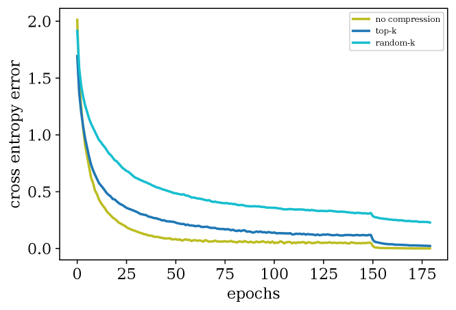
6.4 DL Experiment on CIFAR-10 on Resnet18
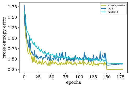
We use the PyTorch framework (Paszke et al., 2019) to empirically compare top- and random- with SGD without compression for training Resnet+BN+Dropout (Resnet18) (He et al., 2016) on the CIFAR-10 dataset (Krizhevsky, 2012). Following the standard practice in compression schemes (Lin et al., 2018; Wang et al., 2018), we apply the compression layer-wise. We use SGD with momentum and we tune the momentum parameter and the learning rate separately for each setting (see Appendix C). Although SGD with momentum is not covered by our analysis, we use this method since it is the state-of-the-art training scheme in deep learning and required to reach a good accuracy. In each setting we trained the neural network for 180 epochs and report the cross entropy error for the training data.
Discussion of results. Figure 6 shows the convergence. We can observe that similar to Figures 2 and 3, top- can still converge to the same error floor as SGD but with a slower rate. Rand- is more severely impacted by the slowdown predicted by theory and would require more iterations to converge to higher accuracy.
7 Conclusion
We provide a convergence analysis of SGD with biased gradient oracles. We reconcile insights that have been accumulated previously, explicitly or implicitly, by presenting a clean framework for the analysis of a general class of biased SGD methods. We show concisely the influence of the bias and highlight important cases where SGD converges with biased oracles. The simplicity of the framework will allow these findings to be broadly integrated, and the limitations we have identified may inspire targeted research efforts that can increase the robustness of SGD.
References
- Aji and Heafield (2017) Alham Fikri Aji and Kenneth Heafield. Sparse communication for distributed gradient descent. In Proceedings of the 2017 Conference on Empirical Methods in Natural Language Processing, pages 440–445. Association for Computational Linguistics, 2017.
- Alistarh et al. (2017) Dan Alistarh, Demjan Grubic, Jerry Li, Ryota Tomioka, and Milan Vojnovic. QSGD: Communication-efficient SGD via gradient quantization and encoding. In NIPS - Advances in Neural Information Processing Systems 30, pages 1709–1720. Curran Associates, Inc., 2017.
- Alistarh et al. (2018) Dan Alistarh, Torsten Hoefler, Mikael Johansson, Nikola Konstantinov, Sarit Khirirat, and Cédric Renggli. The convergence of sparsified gradient methods. In NeurIPS - Advances in Neural Information Processing Systems 31, pages 5977–5987. Curran Associates, Inc., 2018.
- Bach and Perchet (2016) Francis Bach and Vianney Perchet. Highly-smooth zero-th order online optimization. In ALT - 29th Annual Conference on Learning Theory, volume 49 of Proceedings of Machine Learning Research, pages 257–283. PMLR, 2016.
- Baes (2009) Michel Baes. Estimate sequence methods: extensions and approximations. preprint, 2009.
- Bertsekas (2002) Dimitri Bertsekas. Nonlinear Programming. Athena scientific, 2002.
- Beznosikov et al. (2020) Aleksandr Beznosikov, Samuel Horváth, Peter Richtárik, and Mher Safaryan. On biased compression for distributed learning. arXiv preprint arXiv:2002.12410, 2020.
- Bottou et al. (2018) L. Bottou, F. Curtis, and J. Nocedal. Optimization methods for large-scale machine learning. SIAM Review, 60(2):223–311, 2018.
- Bottou (2010) Léon Bottou. Large-scale machine learning with stochastic gradient descent. In Proceedings of COMPSTAT’2010, pages 177–186, 2010.
- Chaturapruek et al. (2015) Sorathan Chaturapruek, John C Duchi, and Christopher Ré. Asynchronous stochastic convex optimization: the noise is in the noise and SGD don’t care. In NIPS - Advances in Neural Information Processing Systems 28, pages 1531–1539. Curran Associates, Inc., 2015.
- Chen and Luss (2018) Jie Chen and Ronny Luss. Stochastic gradient descent with biased but consistent gradient estimators. arXiv preprint arXiv:1807.11880, 2018.
- Chen et al. (2017) Pin-Yu Chen, Huan Zhang, Yash Sharma, Jinfeng Yi, and Cho-Jui Hsieh. ZOO: Zeroth order optimization based black-box attacks to deep neural networks without training substitute models. In Proceedings of the 10th ACM Workshop on Artificial Intelligence and Security, pages 15–26. ACM, 2017.
- d’Aspremont (2008) Alexandre d’Aspremont. Smooth optimization with approximate gradient. SIAM Journal on Optimization, 19(3):1171–1183, 2008.
- Devolder (2011) Olivier Devolder. Stochastic first order methods in smooth convex optimization. CORE Discussion Papers 2011/070, Université catholique de Louvain, Center for Operations Research and Econometrics (CORE), 2011.
- Devolder et al. (2014) Olivier Devolder, François Glineur, and Yurii Nesterov. First-order methods of smooth convex optimization with inexact oracle. Math. Program., 146(1-2):37–75, 2014.
- Dryden et al. (2016) N. Dryden, T. Moon, S. A. Jacobs, and B. V. Essen. Communication quantization for data-parallel training of deep neural networks. In 2nd Workshop on Machine Learning in HPC Environments (MLHPC), pages 1–8, 2016.
- Duchi et al. (2012) John C Duchi, Peter L. Bartlett, and Martin J Wainwright. Randomized smoothing for stochastic optimization. SIAM Journal on Optimization, 22(2):674–701, 2012.
- He et al. (2016) Kaiming He, Xiangyu Zhang, Shaoqing Ren, and Jian Sun. Deep residual learning for image recognition. In 2016 IEEE Conference on Computer Vision and Pattern Recognition, CVPR 2016, Las Vegas, NV, USA, June 27-30, 2016, pages 770–778. IEEE Computer Society, 2016. doi: 10.1109/CVPR.2016.90.
- Hu et al. (2020a) Bin Hu, Peter Seiler, and Laurent Lessard. Analysis of biased stochastic gradient descent using sequential semidefinite programs. Mathematical Programming, 2020a.
- Hu et al. (2016) Xiaowei Hu, Prashanth L. A., András György, and Csaba Szepesvári. (bandit) convex optimization with biased noisy gradient oracles. In Arthur Gretton and Christian C. Robert, editors, Proceedings of the 19th International Conference on Artificial Intelligence and Statistics, AISTATS 2016, Cadiz, Spain, May 9-11, 2016, volume 51 of JMLR Workshop and Conference Proceedings, pages 819–828. JMLR.org, 2016.
- Hu et al. (2020b) Yifan Hu, Siqi Zhang, Xin Chen, and Niao He. Biased stochastic gradient descent for conditional stochastic optimization. arXiv preprint arXiv:2002.10790, 2020b.
- Karimi et al. (2016) Hamed Karimi, Julie Nutini, and Mark Schmidt. Linear convergence of gradient and proximal-gradient methods under the polyak-łojasiewicz condition. In Machine Learning and Knowledge Discovery in Databases, pages 795–811. Springer International Publishing, 2016.
- Karimireddy et al. (2019) Sai Praneeth Karimireddy, Anastasia Koloskova, Sebastian U. Stich, and Martin Jaggi. Efficient greedy coordinate descent for composite problems. In Kamalika Chaudhuri and Masashi Sugiyama, editors, The 22nd International Conference on Artificial Intelligence and Statistics, AISTATS 2019, 16-18 April 2019, Naha, Okinawa, Japan, volume 89 of Proceedings of Machine Learning Research, pages 2887–2896. PMLR, 2019.
- Karimireddy et al. (2018) Sai Praneeth Reddy Karimireddy, Sebastian Stich, and Martin Jaggi. Adaptive balancing of gradient and update computation times using global geometry and approximate subproblems. In AISTATS - Proceedings of the 21st International Conference on Artificial Intelligence and Statistics, volume 84, pages 1204–1213. PMLR, 2018.
- Krizhevsky (2012) Alex Krizhevsky. Learning multiple layers of features from tiny images. University of Toronto, 05 2012.
- Lacoste-Julien et al. (2012) Simon Lacoste-Julien, Mark Schmidt, and Francis Bach. A simpler approach to obtaining an O(1/t) convergence rate for the projected stochastic subgradient method. arXiv e-prints, art. arXiv:1212.2002, Dec 2012.
- Li et al. (2014) Mu Li, David G. Andersen, Alexander J. Smola, and Kai Yu. Communication efficient distributed machinelearning with the parameter server. In NeurIPS, 2014.
- Lin et al. (2018) Yujun Lin, Song Han, Huizi Mao, Yu Wang, and Bill Dally. Deep gradient compression: Reducing the communication bandwidth for distributed training. In 6th International Conference on Learning Representations, ICLR 2018, Vancouver, BC, Canada, April 30 - May 3, 2018, Conference Track Proceedings. OpenReview.net, 2018.
- Liu et al. (2018) Sijia Liu, Bhavya Kailkhura, Pin-Yu Chen, Paishun Ting, Shiyu Chang, and Lisa Amini. Zeroth-order stochastic variance reduction for nonconvex optimization. In NeurIPS - Advances in Neural Information Processing Systems 31, pages 3727–3737. Curran Associates, Inc., 2018.
- Mania et al. (2017) Horia Mania, Xinghao Pan, Dimitris Papailiopoulos, Benjamin Recht, Kannan Ramchandran, and Michael I. Jordan. Perturbed iterate analysis for asynchronous stochastic optimization. SIAM Journal on Optimization, 27(4):2202–2229, 2017.
- Moosavi-Dezfooli et al. (2016) Seyed-Mohsen Moosavi-Dezfooli, Alhussein Fawzi, Omar Fawzi, and Pascal Frossard. Universal adversarial perturbations. arXiv preprints arXiv:1610.08401, 2016.
- Nesterov (2004) Yurii Nesterov. Introductory Lectures on Convex Optimization - A Basic Course, volume 87 of Applied Optimization. Springer, 2004.
- Nesterov and Spokoiny (2017) Yurii Nesterov and Vladimir Spokoiny. Random gradient-free minimization of convex functions. Found. Comput. Math., 17(2):527–566, 2017.
- Niu et al. (2011) Feng Niu, Benjamin Recht, Christopher Re, and Stephen Wright. Hogwild: A lock-free approach to parallelizing stochastic gradient descent. In NIPS - Advances in Neural Information Processing Systems 24, pages 693–701. Curran Associates, Inc., 2011. references refering to arxiv/1106.5730v2 version.
- Nutini et al. (2015) Julie Nutini, Mark Schmidt, Issam Laradji, Michael Friedlander, and Hoyt Koepke. Coordinate descent converges faster with the Gauss-Southwell rule than random selection. In ICML - Proceedings of the 32th International Conference on Machine Learning, pages 1632–1641. PMLR, 2015.
- Paszke et al. (2019) Adam Paszke, Sam Gross, Francisco Massa, Adam Lerer, James Bradbury, Gregory Chanan, Trevor Killeen, Zeming Lin, Natalia Gimelshein, Luca Antiga, Alban Desmaison, Andreas Kopf, Edward Yang, Zachary DeVito, Martin Raison, Alykhan Tejani, Sasank Chilamkurthy, Benoit Steiner, Lu Fang, Junjie Bai, and Soumith Chintala. Pytorch: An imperative style, high-performance deep learning library. In Advances in Neural Information Processing Systems 32, pages 8024–8035. Curran Associates, Inc., 2019.
- Polyak (1987) Boris T. Polyak. Introduction to Optimization. OptimizationSoftware, Inc., 1987.
- Richtárik and Takác (2016) Peter Richtárik and Martin Takác. Parallel coordinate descent methods for big data optimization. Math. Program., 156(1-2):433–484, 2016.
- Schmidt et al. (2011) Mark Schmidt, Nicolas L. Roux, and Francis R. Bach. Convergence rates of inexact proximal-gradient methods for convex optimization. In NIPS - Advances in Neural Information Processing Systems 24, pages 1458–1466. Curran Associates, Inc., 2011.
- Stich (2019) Sebastian U. Stich. Unified optimal analysis of the (stochastic) gradient method. arXiv preprint arXiv:1907.04232, 2019.
- Stich and Karimireddy (2019) Sebastian U. Stich and Sai Praneeth Karimireddy. The error-feedback framework: Better rates for SGD with delayed gradients and compressed communication. arXiv preprint arXiv:1909.05350, 2019.
- Stich et al. (2018) Sebastian U. Stich, Jean-Baptiste Cordonnier, and Martin Jaggi. Sparsified SGD with memory. In NeurIPS - Proceedings of the 32nd International Conference on Neural Information Processing Systems, NIPS’18, pages 4452–4463. Curran Associates Inc., 2018.
- Tappenden et al. (2016) Rachael Tappenden, Peter Richtárik, and Jacek Gondzio. Inexact coordinate descent: Complexity and preconditioning. Journal of Optimization Theory and Applications, 170:144–176, 2016.
- Wang and Giannakis (2020) Gang Wang and Georgios B. Giannakis. Finite-time error bounds for biased stochastic approximation with applications to q-learning. In Silvia Chiappa and Roberto Calandra, editors, The 23rd International Conference on Artificial Intelligence and Statistics, AISTATS 2020, 26-28 August 2020, Online [Palermo, Sicily, Italy], volume 108 of Proceedings of Machine Learning Research, pages 3015–3024. PMLR, 2020.
- Wang et al. (2018) Hongyi Wang, Scott Sievert, Shengchao Liu, Zachary B. Charles, Dimitris S. Papailiopoulos, and Stephen Wright. ATOMO: communication-efficient learning via atomic sparsification. In Samy Bengio, Hanna M. Wallach, Hugo Larochelle, Kristen Grauman, Nicolò Cesa-Bianchi, and Roman Garnett, editors, Advances in Neural Information Processing Systems 31: Annual Conference on Neural Information Processing Systems 2018, NeurIPS 2018, 3-8 December 2018, Montréal, Canada, pages 9872–9883, 2018.
- Wangni et al. (2018) Jianqiao Wangni, Jialei Wang, Ji Liu, and Tong Zhang. Gradient sparsification for communication-efficient distributed optimization. In NeurIPS - Advances in Neural Information Processing Systems 31, pages 1306–1316. Curran Associates, Inc., 2018.
- Zhang et al. (2017) Hantian Zhang, Jerry Li, Kaan Kara, Dan Alistarh, Ji Liu, and Ce Zhang. ZipML: Training linear models with end-to-end low precision, and a little bit of deep learning. In ICML - Proceedings of the 34th International Conference on Machine Learning, volume 70, pages 4035–4043. PMLR, 2017.
Appendix A Deferred Proofs for Section 4
A.1 Proof of Lemma 2
A.2 Proof of Theorem 4
By choosing and , we observe . To see this, assume first that the minimum is attained for . Then we verify
by the choice of . Similarly, if the minimum is attained for , then and
Finally, it remains to note that we do not need to choose smaller than , that is, we cannot get closer than to the optimal solution.
A.3 Proof of Theorem 6
Starting from Equation (6), we proceed by unrolling the recursion and using that for :
Choose the stepsize and . Then we verify:
If the minimum is attained for , then , and it holds
by the choice of . Otherwise, if then
The claim follows again by observing that it suffices to consider only. .
Appendix B Deferred Proofs for Section 5
B.1 Top- sparsification
Definition 3.
For a parameter , the operator is defined for as:
where is a permutation of such that for . In other words, the operator keeps only the largest elements of a vector and truncates the other ones to zero.
We observe that for the operator, we have
| (9) |
and both inequalities can be tight in general.
Lemma 9.
Let we differentiable, then is a -biased gradient oracle for
Proof.
This follows directly from (9). ∎
B.2 Random- sparsification
Definition 4.
For a parameter , the operator , where denotes the set of all element subsets of , is defined for as:
where is a set of elements chosen uniformly at random from , i.e, .
We observe that for the operator, we have
| (10) |
and further
| (11) |
for any vectors . Moreover
| (12) |
Lemma 10.
Let be an unbiased gradient oracle with -bounded noise. Then is a -biased gradient oracle with -bounded noise, for
Proof.
The gradient oracle can be written as , for -bounded noise. We first estimate the bias
where we used independence to conclude .
For the noise, we observe , and hence
the statement of the lemma follows. ∎
Remark 11.
These bounds are tight in general. When , then we just recover , . For the special case when , then we recover and , i.e, the randomness of the oracle would be only due to the random- sparsification.
Biased versus unbiased sparsification.
In the literature, often an unbiased version of random sparsification is considered, namely the scaled operator .
Up to the scaling by , the operator is therefore identical to the operator, and we would expect the same convergence guarantees, in particular with tuning for the optimal stepsize (as in our theorems). However, due to the constraint as a consequence of applying the smoothness in Lemma 2, this rescaling might not be possible if (only if it is smaller). This is the reason, why the lemma below gives a slightly better estimate for the convergence with than with (the optimization term, the term not depending on , is improved by a factor ).
However, we argue that this is mostly a technical issue, and not a limitation of vs. . Our Lemma 2 does not assume any particular structure on the bias and holds for arbitrary biased oracles. For the particular choice of , we know that scaling up the update by a factor is possible in any case, and hence the condition on the stepsize could be relaxed to in this special case—recovering exactly the same convergence rate as with .
Lemma 12.
Let be an unbiased gradient oracle with -bounded noise. Then is a -biased gradient oracle with -bounded noise, for
Proof.
The unbiasedness is easily verified. For the variance, observe
B.3 Zeroth-Order Gradient
Lemma 13.
Proof.
From Nesterov and Spokoiny (2017, Lemma 3) we can bound the bias for as follows:
Hence we can conclude that Assumption 4 holds with the choice , and . Moreover, Nesterov and Spokoiny (2017, Theorem 4) provide an upper bound on the second moment of the zeroth-order gradient oracle :
The second moment is an upper bound on the variance. Hence we can conclude that Assumption 3 hold with the choice
Convergence rate for under PL condition.
Using the result from Theorem 6, we can conclude that under PL condition,
iterations is sufficient for zeroth-order gradient descent to reach . Observe that for any reasonable choice of , the second term is of order only, and hence the rate is dominated by the first term. We conclude, that zeroth-order gradient descent requires iterations to converge to the accuracy level of the bias term which cannot be surpassed.
The convergence rate matches with the rate established in (Nesterov and Spokoiny, 2017, Theorem 8), but in our case the convergence radius (bias term) is times worse than theirs. This shows that in general the rates given in Theorem 6 can be improved if stronger assumptions are imposed on the bias term or if it is known how the gradient oracle (and bias) are generated, for instance by Gaussian smoothing.
B.4 Inexact gradient oracle
First, we give the definition of a oracle as introduced in (Devolder et al., 2014).
Definition 5 (()-oracle (Devolder et al., 2014)).
Let function be convex on , where is a closed convex set in . We say that is equipped with a first-order -oracle if for any we can compute a pair such that:
The constant is called the accuracy of the oracle. A function is -smooth if and only if it admits a -oracle. However the class of functions admitting a -oracle is strictly larger and includes non-smooth functions as well.
Stochastic inexact gradient oracle.
Devolder (2011) generalized the notion of -gradient oracle to the stochastic case. Instead of using the pair , they use the stochastic estimates such that:
where is a -oracle as defined above. From the third inequality we can conclude that . Moreover the bias term can be upper bounded by:
Therefore we can conclude that , and .
B.5 Biased compression operators
Appendix C Details on the deep learning experiment
The hyper-parameter choices used in our deep learning experiments (Section 6.4) are summarized in Table 2. We tuned the hyper-parameters over the range for learning rate and for momentum and choose the combination of hyper-parameters that gave the least test error. In all of the settings we reduced the learning rate at the epoch 150 with a factor of 10 and we trained the network with a batch size of and a penalty regularizer equal to .
| method | lr | momentum | ||
|---|---|---|---|---|
| SGD | 0.1 | 0.9 | ||
| top- | 0.1 | 0.75 | ||
| rand- | 0.1 | 0.75 |