On the convergence of an improved and adaptive kinetic simulated annealing
Abstract.
Inspired by the work of Fang et al. (1997), who propose an improved simulated annealing algorithm based on a variant of overdamped Langevin diffusion with state-dependent diffusion coefficient, we cast this idea in the kinetic setting and develop an improved kinetic simulated annealing (IKSA) method for minimizing a target function . To analyze its convergence, we utilize the framework recently introduced by Monmarché (2018) for the case of kinetic simulated annealing (KSA). The core idea of IKSA rests on introducing a parameter , which de facto modifies the optimization landscape and clips the critical height in IKSA at a maximum of . Consequently IKSA enjoys improved convergence with faster logarithmic cooling than KSA. To tune the parameter , we propose an adaptive method that we call IAKSA which utilizes the running minimum generated by the algorithm on the fly, thus avoiding the need to manually adjust for better performance. We present positive numerical results on some standard global optimization benchmark functions that verify the improved convergence of IAKSA over other Langevin-based annealing methods.
AMS 2010 subject classifications: 60J25, 60J60, 46N30
Keywords: simulated annealing; Langevin diffusion; relative entropy; log-Sobolev constant; self-interacting diffusion; landscape modification
1. Introduction
Given a target function to minimize, we are interested in simulated annealing algorithms based on Langevin diffusion and its various variants. Let us begin by briefly recalling the dynamics of the classical overdamped Langevin diffusion for simulated annealing (SA):
| (1.1) |
where is the standard -dimensional Brownian motion and is the temperature or cooling schedule. The instantaneous stationary distribution of (1.1) at time is the Gibbs distribution that we denote by
We shall explain the seemingly strange upper script that appears in later in (1.6). This overdamped Langevin dynamics and its convergence have been analyzed in Chiang et al. (1987); Holley et al. (1989); Miclo (1992); Jacquot (1992). It can be shown that under the logarithmic cooling schedule of the form
| (1.2) |
where , gradually concentrates around the set of global minima of in the sense that for any ,
Here we write . We call the energy level and the hill-climbing constant or the critical height associated with . Intuitively speaking, is the largest hill one need to climb starting from a local minimum to a fixed global minimum. For a precise definition of , we refer readers to (2.2) below.
While the overdamped Langevin diffusion (1.1) can be seen as the continuous counterpart of gradient descent perturbed by Gaussian noise, the analogue of momentum method in this context is the kinetic or underdamped Langevin diffusion. The kinetic Langevin dynamics (KSA) is described by
| (1.3) | ||||
| (1.4) |
where stands for the position and is the velocity or momentum variable. The instantaneous stationary distribution of at time is the product distribution of and the Gaussian distribution with variance that we denote by
We will explain the notation in (1.10) below. Unlike the overdamped Langevin dynamics (1.1) which is reversible, the kinetic counterpart (1.3) is in general non-reversible, which imposes technical difficulties in establishing its long-time convergence. On the other hand, it is known in the literature that using non-reversible dynamics may accelerate convergence in the context of sampling or optimization, see for example Diaconis et al. (2000); Bierkens (2016); Chen and Hwang (2013); Löwe (1997); Duncan et al. (2016, 2017); Hwang et al. (2005); Gao et al. (2018); Hu et al. (2020). Using a distorted entropy approach, in Monmarché (2018) the author proves for the first time convergence result of kinetic simulated annealing: under the same logarithmic cooling schedule as in (1.2), for any we have
More recently, Chak et al. (2020) analyze the generalized Langevin dynamics for simulated annealing based on the framework introduced in Monmarché (2018).
Many techniques have been developed in the literature to improve or to accelerate the convergence of Langevin dynamics. In this paper, we are particularly interested in an improved variant of Langevin dynamics (ISA) with state-dependent diffusion coefficient, introduced by Fang et al. (1997), and its dynamics is described by the following:
| (1.5) |
where we write for . Comparing the improved dynamics (1.5) with the classical one (1.1), we see that the function and the parameter are introduced. We formally state the assumptions needed on both and in Assumption 1.1 below. To briefly summarize, we need to choose and to be twice-differentiable, non-negative, bounded and non-decreasing with . It is shown in Fang et al. (1997) that the instantaneous stationary distribution at time of (1.5) is given by
| (1.6) |
where
| (1.7) |
Observe that if , (1.5) reduces to the classical overdamped dynamics (1.1). As such can be considered as a generalization of the Gibbs distribution . This also explains the notation earlier.
One important difference between (1.5) and (1.1) is the introduction of state-dependent diffusion coefficient: the greater the difference between and , the greater (in absolute terms) the Gaussian noise is to be injected, and this extra noise may improve the convergence by helping the dynamics to escape a local minimum or saddle point. On the other hand, in the region where the dynamics evolves in the same manner as the classical dynamics. As for the theoretical benefits, in Fang et al. (1997) the authors demonstrate that under the logarithmic cooling schedule of the form (1.2) with and for any ,
where we call the clipped critical height, to be defined formally in (2.3) below. It can be shown that and , and hence one can understand as if the critical height is capped at a maximum level . The key technical insight in Fang et al. (1997) relies on both the spectral gap and the log-Sobolev constant are of the order . As a result, we can operate a faster cooling schedule for the improved dynamics (1.5) that still enjoys convergence guarantee.
The crux of this paper is to cast the idea of Fang et al. (1997) into the kinetic Langevin setting for simulated annealing. One way to do so is to think of altering the target function: in SA the exponent in is , while in ISA the exponent in (1.6) takes on the generalized form as . In this way the optimization landscape is de facto modified from to and hopefully improved. We apply this idea and simply substitute by in its dynamics. More precisely, we are interested in the following dynamics that we call IKSA:
| (1.8) | ||||
| (1.9) |
Its instantaneous stationary distribution at time is the product distribution of and the Gaussian distribution with mean and variance :
| (1.10) |
Note that when , , and we retrieve exactly the classical kinetic Langevin diffusion (1.3). As such we can think of IKSA as a generalization of KSA. This also explains the notation that appears earlier.
For a general (that satisfies Assumption 1.1 below), in the case of we have , and hence the improved kinetic dynamics (1.8) evolves in the same way as the classical one (1.3) in this region. In the other case when , we see that
Thus, the greater is relative to , the greater the denominator in in the above equation, and the more dominant is the Brownian noise in the velocity update of . This effect can hopefully improve the convergence of when its value is greater than . To illustrate, we plot the following function
as in Monmarché (2018) and compare this landscape with that of in Figure 1, where we take , and . For example, when in Figure 1, we can see that the gradient of is much smaller than that of , thus the Brownian noise plays a relatively more dominant role in this region in the velocity update. While it may not be immediately apparent in Figure 1, we note that both (the black and solid curve) and (the orange and dashed curve) share exactly the same set of stationary points. As for the theoretical advantage of using IKSA, we shall prove that we can operate a faster logarithmic cooling schedule than KSA, relying on the key technical insight that the instantaneous spectral gap and the log-Sobolev constant are of the order .
While there are practical benefits in using IKSA over KSA or ISA over SA, on the other hand they come along with extra computational costs: in the velocity update of IKSA, in addition to evaluating the gradient of , we would need to evaluate both and its derivative at , as the core idea of IKSA or ISA rests on comparing and for all . As such if we implement the Euler-Maruyama discretization of IKSA, extra function evaluations are required at each iteration.
The objective of this paper is to promote the idea of landscape modification and state-dependent noise in stochastic optimization. It has been brought to us by Miclo (2020) that Olivier Catoni has also considered the operation from to in a discrete-time and finite state space setting with concave . Recently in Guo et al. (2020) the authors study perturbed gradient descent with state-dependent noise, using the notion of occupation time.

We summarize the main contributions of this paper below:
-
(1)
Propose an improved kinetic simulated annealing (IKSA) method and analyze its convergence
In our main result Theorem 1.1 below, we will prove that under the logarithmic cooling of the form (1.2) with energy level , where both and are fixed, the improved kinetic annealing converges: for any ,
This will be proved using the framework proposed by Monmarché (2018), along with the key technical insight that the log-Sobolev constant is of the order at time .
-
(2)
Propose an adaptive (IAKSA) method to tune the parameter and the energy level , and analyze its convergence
The convergence behaviour of in IKSA highly depends on the value of the parameter . Ideally we would like to choose to be close to (so that the clipped critical height is as small as possible), but it can be hard to achieve in practice without a priori information on .
In our second main result Theorem 1.2 below, we tune both and adaptively by incorporating the information of the running minimum , where both and depend on the running minimum generated by the algorithm on the fly. We call the resulting non-Markovian diffusion IAKSA. Although the setting is slightly different, this idea is in reminiscence of the adaptive biasing method Benaïm and Bréhier (2019); Benaïm et al. (2020); Lelièvre and Minoukadeh (2011); Lelièvre et al. (2008) or the self-interacting annealing method Raimond (2009), thus avoiding the need to manually tune the parameter for better performance. We also mention the related work of memory gradient diffusions Gadat et al. (2013); Gadat and Panloup (2014). Adaptive algorithms are popular in the Markov chain Monte Carlo (MCMC) literature as well Roberts and Rosenthal (2009); Andrieu and Thoms (2008); Fort et al. (2011). Note that in our context, the idea of tuning adaptively on the fly dates back to the work Fang et al. (1997) for ISA.
-
(3)
Present numerical experiments to illustrate the performance of IAKSA
We compare the performance of four simulated annealing methods, namely IAKSA, IASA (1.5) (i.e. ISA with the parameter tuned adaptively in the same way as IAKSA), KSA (1.3) and SA (1.1), on minimizing three standard global optimization benchmark functions Jamil and Yang (2013). Empirical results demonstrate the improved convergence performance of IAKSA over other annealing methods that are based on Langevin diffusions.
1.1. Notations
Before we discuss our main results, we fix a few notations that are frequently used throughout the paper. For , we write and . For , we write to be its Euclidean norm. We also denote by to be the partial derivative with respect to . For two functions on , we write if there exists constant such that for large enough . We write if . We also use the little-o notation: if . We say that a function is a subexponential function if .
In the rest of the paper, as is fixed, we shall hide its dependence on various quantities. We will write and .
1.2. Overview of the main results
In this subsection, we state our main results. First, let us clearly state the assumptions on the target function , the function and the parameter . Note that the critical height and clipped critical height will be introduced in Section 2.3. These assumptions are standard in the simulated annealing literature.
Assumption 1.1.
-
(1)
The potential function is smooth with bounded second derivatives, that is,
Also, there exist constants such that satisfies
where .
-
(2)
The function is twice-differentiable, bounded, non-negative and non-decreasing. Furthermore, satisfies
and there exist constant such that
We also denote .
-
(3)
The cooling schedule satisfies, for large enough ,
This is for instance satisfied by the logarithmic cooling schedule (1.2).
-
(4)
The parameter is picked so that . In the adaptive case, for all .
-
(5)
The initial law of admits a smooth density with respect to the Lebesgue measure that we denote by . Its Fisher information and moments are all finite, where .
Our first main result gives large-time convergence guarantee for IKSA , introduced earlier in (1.8):
Theorem 1.1.
[Convergence of IKSA] Under Assumption 1.1, for any , as we have
If we employ the logarithmic cooling schedule of the form for large enough , where , and both and are fixed, then for any , there exists constant such that
| (1.11) |
If we compare the result of Monmarché (2018) for KSA (1.3) against the result we obtain in Theorem 1.1 for IKSA (1.8), in essence we replace the critical height by the clipped critical height . In retrospect this is perhaps unsurprising, as one can understand the modification in IKSA as clipping the target function from to . While IKSA enjoys improved logarithmic cooling when compared with KSA, logarithmic cooling is however known to be inefficient, see Catoni (1992) and the Remark in (Monmarché, 2018, Section ).
In our second main result, we propose an adaptive method, that we call IAKSA, to tune the parameter and the energy level using the running minimum on the fly. We shall discuss in more technical details in Section 3. Note that the idea of tuning adaptively on the fly dates back to the work Fang et al. (1997) for ISA.
Theorem 1.2.
[Convergence of IAKSA] Under Assumption 1.1, consider the kinetic dynamics described by
where is introduced in (1.7), is tuned adaptively according to (3.1) and the cooling schedule is
with satisfying (3.2). Given , for large enough and a constant , we consider sufficiently small such that , and select such that , to yield
where
1.3. Numerical results
In this subsection, we present our numerical illustrations. The benchmark functions are the Rastrigin function , Ackley3 function and Ackley function . For further details on the experimental setup and the parameters used (such as initialization, stepsize or the cooling schedule), these are described in the Appendix.
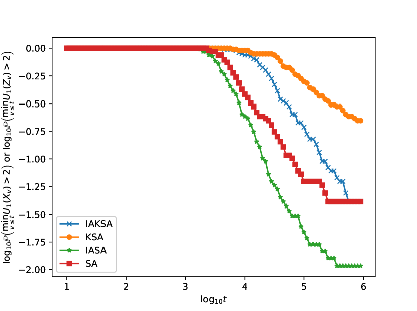
We mimic Figure in Monmarché (2018), and we plot the corresponding results in Figure 2 for the three benchmark functions. On the vertical axis, we plot or against in Figure (2(a)), (2(c)) and (2(e)), and similarly we plot or against in Figure (2(b)), (2(d)) and (2(f)). To compute these probabilities, we run 100 independent replicas and count the proportion of replicas for which or . We inject the same sequence of Gaussian noise in each of the 100 replicas across all four annealing methods for fair comparison.
KSA and SA can be considered as the baseline algorithms for IAKSA and IASA respectively. In all of the plots in Figure (2) IAKSA outperforms KSA, revealing that there is perhaps empirical advantage in using IAKSA over classical KSA in some instances.
For the Rastrigin function in Figure (2(a)) and (2(b)), we note that IAKSA enjoys improved convergence over other methods, while SA does not seem to converge near at all. For IASA and KSA, although their running minimum reach the neighbourhood of when is approximately 3 to 5, as evident from Figure (2(b)) they however do not get stuck at the neighbourhood.
For the Ackley3 function in Figure (2(c)) and (2(d)), we first observe that the curve corresponding to the running minimum of IASA drops fast but stays flat when is bigger than 5. In Figure (2(d)), the only method that lingers around the neighbourhood of is IAKSA.
For the Ackley function in Figure (2(e)) and (2(f)), the two overdamped methods IASA and SA seem to outperform the two kinetic methods IAKSA and KSA.


1.4. Organization of the paper
2. Proof of Theorem 1.1
In this section, we prove the convergence of the improved kinetic dynamics with fixed and energy level . We employ the same proof strategy as in Monmarché (2018) and break down the proof into smaller parts. Finally, in Section 2.8 we connect the auxiliary results and finish off the proof of Theorem 1.1.
2.1. Weak convergence of
In this subsection, we prove that converges weakly to the set of global minima of as . Recall that is first introduced in (1.6) as the stationary distribution of the improved annealing ISA method. Note that similar result have been obtained in Fang et al. (1997).
Proposition 2.1.
Under Assumption 1.1, for a fixed , suppose the law of is . Then for sufficiently small with , there exists a constant , independent of , such that
[Proof. ]First, denote . For any Borel set , we denote to be its Lebesgue volume. Note that an equivalent way of writing down is
where the set is compact as is quadratic at infinity. Define
Note that under Assumption 1.1, since is quadratic at infinity, the set is compact. Therefore, we have
2.2. Existence and regularity for the density of IKSA
First, we note that the infinitesimal generator of the improved kinetic dynamics (1.8) at a fixed temperature is
| (2.1) |
where we recall is first introduced in (1.7), and (resp. ) is the divergence operator with respect to the variable (resp. ). When there is no ambiguity on the parameter , we simply hide the dependency on and write and .
We show that the density of is nice:
Proposition 2.2.
Under Assumption 1.1, the process is well-defined and the second moment is finite for all . The Lebesgue density of , denoted by , is smooth and positive.
is well-defined and smooth.
[Proof. ]We follow the same proof as in (Monmarché, 2018, Proposition 4 and 5).
First, we show the non-explosiveness and the finite second moment result. Consider the homogeneous Markov process , its generator and Hamiltonian function
Note that for :
where the constant depends the bounds of and its derivative on . Using the Markov inequality and the Ito’s formula, we have which implies that the second moment is finite.
For the smoothness of , one can readily check the Hormander’s bracket condition is satisified.
For the positiveness of , we apply exactly the same argument as in Proposition of Monmarché (2018), with therein replaced by .
2.3. The log-Sobolev inequality
In this subsection, we prove the log-Sobolev inequality for the improved kinetic Langevin process . First, let us briefly recall the concept of critical height that frequently appears in various classical and modern work of the annealing literature Jacquot (1992); Holley and Stroock (1988); Miclo (1992). For two points we write to be the set of parametric curves that start at and end at . Given a target function , the classical critical height of is then defined to be
| (2.2) |
One major motivation of the current work is the introduction of the function and the parameter that control the injection of the Gaussian noise into the system, which allows one to clip the critical height at an arbitrary level , thus effectively reducing . Precisely, for an arbitrary and , we define to be
| (2.3) |
For probability measure on and smooth positive function on such that , we define the relative entropy and Fisher information to be respectively
Proposition 2.3.
Under Assumption 1.1 and suppose the temperature is fixed. For any arbitrary and positive smooth function with , there exists and a polynomial function (which may depend on ) such that
Remark 2.1.
In Fang et al. (1997), by introducing assumption on the behaviour of near (Assumption therein), they demonstrate the log-Sobolev constant is of the order , while in our Assumption 1.1, we do not place such assumption on , at the trade-off of introducing an error that appears in . Alternatively, we can insert extra assumptions and simply use the result obtained in Fang et al. (1997) for the log-Sobolev inequality.
[Proof. ]First, note that can be written as a tensor product of (for the coordinates) and a Gaussian distribution of mean with variance (for the coordinates). Since the log-Sobolev inequality tensorizes and is stable under perturbation (see e.g. the references as in Monmarché (2018); Chak et al. (2020)), it suffices for us to determine the log-Sobolev constant of .
Let us recall the improved overdamped Langevin dynamics at temperature is described by the dynamics
with generator and -spectral gap
where we write to be the inner product in for . Define
Since , we thus have
Therefore, we can pretend our target function is at temperature in the classical Langevin dynamics, and utilize the result of Jacquot (1992) to conclude that, for a constant independent of ,
| (2.4) |
If we show that
| (2.5) |
where is a constant that depends on and but not on , the desired result follows from the above spectral gap estimate and (Fang et al., 1997, Theorem ).
In order to apply the result of Jacquot (1992), we check Condition and therein:
-
•
Condition : and as since is quadratic at infinity.
-
•
Condition : Outside the ball of ,
and so is bounded below outside the ball , and hence it is bounded below for all .
Now, we observe that, for any ,
Writing to be the ball center at with sufficiently large radius , we finally show (2.5):
2.4. Lyapunov function and moment estimates
The aim of this section is to prove the following moment estimate of :
Proposition 2.4.
For any , and large enough (which depends on and the temperature schedule ), there exist a constant , independent of , such that
We first prove the following Lyapunov property in Section 2.4.1, followed by proving Proposition 2.4 in Section 2.4.2.
Proposition 2.5 (Lyapunov property of ).
Let
| (2.6) |
For , there exist constants and a subexponential function of such that
2.4.1. Proof of Proposition 2.5
As we have
summing up these two equations leads to
| (2.7) |
Note that we also have
| (2.8) |
We proceed to give an upper bound on the second and the third term in the above equation. We first consider lower bounding :
| (2.9) |
where the first inequality follows from Assumption 1.1 item 1, and we recall both and are introduced in Assumption 1.1 item 2. Next, as we have
dividing by leads to
| (2.10) |
We substitute (2.4.1) and (2.10) into (2.8) to yield
| (2.11) |
The next two results give upper and lower bounds for and .
Lemma 2.1.
For any , the upper bound of is
Consequently, we have
On the other hand, the lower bound of is
Consequently, we have
[Proof. ]We shall only prove the bounds on , and from these bounds it is straightforward to deduce the bounds on . We first prove the upper bound of . If , we have
where the second inequality follows from the assumption on in Assumption 1.1. If ,
where the inequality follows from Assumption 1.1 again. For the lower bound of , we consider
where the second inequality follows from Assumption 1.1.
Lemma 2.2.
For the upper bound of , we have
On the other hand, the lower bound of is
Using Lemma 2.1 together with (2.4.1) leads to, for some constants ,
and hence, when combined with (2.7) and (2.6),
Finally, the above equation together with Lemma 2.2 gives, for some constants and a subexponential function of ,
2.4.2. Proof of Proposition 2.4
Proposition 2.6.
For any and , there exist subexponential functions such that
[Proof. ]For some constants , we compute
Now, we use the lower bound of in Lemma 2.2 to see that
and so
The carré du champ operator of is . Using the lower bound of in Lemma 2.2, we compute, for constant and subexponential functions ,
| (2.12) |
Proposition 2.7.
For any , and large enough , there exist a constant such that
[Proof. ]We shall prove the result by induction on . We denote by . When , the result clearly holds. When , using Proposition 2.5 and 2.6 we have
As , and for any as , we deduce that, for constants ,
| (2.13) |
As a result, for constant ,
This proves the result when . Assume that the result holds for all , where . First, using Proposition 2.5 and equation (2.4.2) we compute
| (2.14) |
Differentiating with respect to , followed by using Proposition 2.6 and equation (2.4.2) give
where we use the same asymptotic estimates that lead us to (2.13) and the induction assumption on and .
Now, we wrap up the proof of Proposition 2.4.
Using the lower bound of in Lemma 2.2, we note that, for some constants and arbitrary ,
where the equality follows from the binomial theorem, the second inequality follows from the Jensen’s inequality, the third inequality comes from Proposition 2.7, and we use the estimates , for large enough in the last inequality.
2.5. Gamma calculus
For smooth enough and , as is a diffusion, recall that we have
where is the carré du champ operator with Let be the adjoint of , that is,
For a non-negative function from to which belongs to some functional space , and a differentiable with differential operator , the directional derivative in , we will be interested in quantities of the form
| (2.15) |
We now present three auxiliary lemmas, which are essential in proving the dissipation of the distorted entropy later in Section 2.7. The proofs are essentially the same as corresponding proofs in Monmarché (2018), by replacing the target function therein with .
Lemma 2.3.
For non-negative and , then
[Proof. ]The proof is the same as (Monmarché, 2018, Lemma ), by replacing the target function therein with .
Lemma 2.4.
For non-negative and , where is a linear operator from to , then
where for two operators , the commutator bracket is , and .
[Proof. ]The proof is the same as (Monmarché, 2018, Lemma ), by replacing the target function therein with .
Lemma 2.5.
Let
We have
[Proof. ]The proof is the same as (Monmarché, 2018, Corollary ), by replacing the target function therein with .
2.6. Truncated differentiation
In this subsection, we present auxiliary results related to mollifier and truncated differentiation. These results are needed when we discuss the dissipation of distorted entropy in Section 2.7 below.
Let be a mollifier defined to be
For , we define
| (2.16) | ||||
| (2.17) |
where is the convolution of two functions and is the indicator function of the set . Recall that in Lemma 2.2 the lower bound of is given by
Denoting the third term on the right hand side by
we define, for any and ,
| (2.18) |
Note that for large enough (which depends on and the cooling schedule ), for all . Also, note that can be negative as may possibly be negative. With our choice of it ensures that .
Now, we present results that summarize some basic properties of .
Lemma 2.6.
For ,
-
(1)
is compactly supported;
-
(2)
converges to pointwise;
-
(3)
For some constant , independent of and time , we have, for large enough ,
[Proof. ]Similar to Chak et al. (2020), we have the following estimates:
From these it is straightforward to show item (1) and (2). We proceed to prove item (3). First, using Gamma calculus and the above upper bounds on , we have, for some constant ,
where the last inequality follows from the Lyapunov property of in Proposition 2.5. Now, we bound each of the two terms on the right hand side above. Using and , we observe that
where we use as in Proposition 2.5 and .
For the second term, using
and the lower bound of in Lemma 2.2 again,
we see that, for some constant ,
which can clearly be bounded above independent of .
2.7. Dissipation of the distorted entropy
Recall the notation in Section 2.2 that is the density of the process at time with respect to the distribution . For non-negative , we define the functionals
and we recall that in Lemma 2.5 we introduce
With these notations in mind we define the distorted entropy as, for ,
| (2.19) |
The distorted entropy is not to be confused with introduced in (1.7). In order to compute the time derivative of the distorted entropy and pass the derivative into the integral, we will first be working with its truncated version, which is defined to be, for ,
| (2.20) |
where we recall is the mollifier introduced in (2.18). Taking the time derivative of (2.20) and thanks to Lemma 2.6, we have
| (2.21) |
We will handle and give upper bound on each of the two terms on the right hand side above separately.
For the first term on the right hand side of (2.21), we have the following upper bound:
Lemma 2.7.
For the same constant that appears in Lemma 2.6,
[Proof. ]
where the third equality follows from (Chak et al., 2020, discussion below ) and the fourth equality comes from classical Gamma calculus as in (2.15). For the fifth equality, we add to ensure that . For the last inequality, we make use of Lemma 2.5 for the first term and Lemma 2.6 for the second term.
We proceed to consider the second term on the right hand side of (2.21). Using the chain rule, we have
| (2.22) |
where the second equality follows from the proof in Lemma 2.6. Now, as in the proof of (Monmarché, 2018, Lemma ), we compute that
Using the quadratic growth assumption on in Assumption 1.1, there exist a subexponential function such that
| (2.23) |
Lemma 2.8.
There exist subexponential function such that
[Proof. ]
where we use in the equality, and in the inequality we utilize as well as (2.23). Next, for matrix since , we consider
where the inequality follows again from (2.23). The desired result follows from taking
We write the Fisher information at time to be
Collecting the results of Lemma 2.7, (2.7) and Lemma 2.8 and substitute these back into (2.21), we obtain the following:
Proposition 2.8.
[Proof. ]First, according to the results of Lemma 2.7, (2.7) and Lemma 2.8, we put these back into (2.21) to obtain
Integrating from to leads to
The desired result follows by taking , Fatou’s lemma and Lemma 2.6.
Finally, the objective of this section is to prove the following bound on the distorted entropy:
Proposition 2.9.
Under Assumption 1.1, we have, for any , there exists constant such that for large enough ,
[Proof. ]The proof mimics that of (Monmarché, 2018, Lemma ), except that we have an improved estimate of the log-Sobolev constant in our setting. More precisely, using the log-Sobolev inequality Proposition 2.3 and Proposition 2.8 we have
| (2.24) |
where we recall is a subexponential function, and is first introduced in Proposition 2.3.
First, we handle the second term in (2.7). Using , Proposition 2.4 and for large enough and any leads to
| (2.25) |
Next, we consider the first term in (2.7). Using the fact that is polynomial in leads to
| (2.26) | ||||
| (2.27) |
Collecting the results of (2.25), (2.27) and (2.26) and put these back into (2.7), if we choose small enough, there exists constants such that
The rest of the proof follows exactly that of (Monmarché, 2018, Lemma ) (with therein replaced by our ), which further relies on the estimate obtained in (Miclo, 1992, Lemma ).
2.8. Wrapping up the proof
In this subsection, we finish off the proof of Theorem 1.1 by using the auxiliary results obtained in previous sections.
3. An adaptive algorithm (IAKSA) and its convergence
Throughout this section, we assume that for the ease of calculation.
Recall that in IKSA, introduced in Theorem 1.1, the performance of the diffusion depends on the parameter . In this section, we propose an adaptive method to tune both the parameter and the energy level . First, we rewrite the dynamics of to emphasize the dependence on and :
where is introduced in (1.7). The parameter and the cooling schedule are tuned adaptively using the running minimum . Recall that for , is a mollifier introduced in Section 2.6. In the following we shall use the mollifier with support on . We tune the parameter adaptively by setting
| (3.1) |
and hence, according to the definition of in (2.3), for arbitrary an upper bound of is given by
Let . Now, the energy level that appears on the numerator of the cooling schedule is also tuned adaptively:
| (3.2) |
As we shall see in the proof, the primary reason of mollifying allows us to consider the derivative of or with respect to time , and the choice of using is arbitrary. This is essential in analyzing the dissipation of the distorted entropy. For instance, we need to consider the time derivative of the cooling schedule, and as such we have to ensure that is differentiable.
For the convenience of readers, we restate Theorem 1.2 below:
Theorem 3.1.
Under Assumption 1.1, consider the kinetic dynamics described by
where is introduced in (1.7), is tuned adaptively according to (3.1) and the cooling schedule is
with satisfying (3.2). Given , for large enough and a constant , we consider sufficiently small such that , and select such that , to yield
where
The rest of this section is devoted to the proof of Theorem 1.2.
3.1. Dissipation of the distorted entropy in the adaptive setting
In this subsection, we present some auxiliary results which will be used in Section 3.2, the proof of Theorem 1.2. In a nutshell, we show that under appropriate assumptions on and , key results such as Proposition 2.9 also hold in this adaptive setting:
Proposition 3.1.
Under Assumption 1.1, suppose further that the parameter is tuned adaptively by and the energy level is , which are non-increasing with respect to time. We write as in (2.3), and we assume that
For sufficiently small with for all , there exists constant such that for large enough ,
Note that both and are possibly time-dependent.
Remark 3.1.
In Section 3.2, we show that such a choice of is possible.
The rest of this subsection is devoted to the proof of Proposition 3.1.
3.1.1. Auxiliary results
In this subsection, we present five auxiliary results which will be used in the proof of Proposition 3.1, namely Lemma 3.1, Proposition 3.2, Proposition 3.3 and Proposition 3.4.
First, to emphasize the dependence of on various quantities, compared with (2.20) the truncated distorted entropy is now written as
where we note that the stationary distribution depends on and depends on through . Taking the derivative with respect to gives
| (3.3) | ||||
Comparing with (2.21), the extra term in (3.3) vanishes when for all . The first two terms in (3.3) can be handled in exactly the same way as in Lemma 2.7, equation (2.7) and Lemma 2.8. We proceed to simplify the third term in (3.3). We note that
| (3.4) | ||||
where we use Assumption 1.1 in the first inequality. The above computation leads to
| (3.5) |
where is a subexponential function of . Our first auxiliary result handles the third term in (3.3).
Lemma 3.1.
There exist subexponential function such that
[Proof. ]
where we use in the equality, and in the inequality we utilize as well as (3.5). Next, for matrix since , we consider
where the inequality follows again from (3.5).
Next, we consider the time derivative of the distorted entropy. The result is essentially the same as Proposition 2.8 for the case of fixed , except that in the adaptive setting we have to introduce and its time derivative:
Proposition 3.2.
There exist subexponential function such that
[Proof. ]First, according to the results of Lemma 2.7, (2.7), Lemma 2.8 and Lemma 3.1, we put these back into (3.3) to obtain
Integrating from to leads to
The desired result follows by taking , Fatou’s lemma and Lemma 2.6.
Our next two results generalize Proposition 2.7 and Proposition 2.4 respectively to the adaptive setting.
Proposition 3.3.
Under the same assumptions as in Proposition 3.1, for any , and large enough , there exist a constant such that
[Proof. ]We shall prove the result by induction on . We denote by . When , the result clearly holds. When , using Proposition 2.5 and 2.6 we have
where we use (3.4) in the first inequality. As , and
for any as , we deduce that, for constants ,
| (3.6) |
The rest of the argument is the same as Proposition 3.3. This proves the result when . Assume that the result holds for all , where . First, using Proposition 2.5 and equation (2.4.2) we compute
Differentiating with respect to , followed by using Proposition 2.6 and equation (2.4.2) give
where we use the same asymptotic estimates that lead us to (3.6) and the induction assumption on and .
Proposition 3.4.
Under the same assumptions as in Proposition 3.1, for any , and large enough (which depends on and the temperature schedule ), there exist a constant such that
3.1.2. Proof of Proposition 3.1
Using the log-Sobolev inequality Proposition 2.3 and Proposition 3.2 we have
| (3.7) |
where we recall is a subexponential function, and is first introduced in Proposition 2.3.
First, we handle the second term in (3.1.2). Note that
Using , Proposition 2.4 and for large enough and any leads to
| (3.8) |
Next, we consider the first term in (3.1.2). Using the fact that is polynomial in and lead to
| (3.9) | ||||
| (3.10) |
Collecting the results of (3.8), (3.10) and (3.9) and put these back into (3.1.2), if we choose small enough, there exists constants such that
The rest of the proof follows exactly that of (Chak et al., 2020, Equation to ), and we need to check that, as to ,
3.2. Proof of Theorem 1.2
First, we check that with our choice of in (3.1) and in (3.2), the assumptions in Proposition 3.1 are satisfied:
[Proof. ]Clearly, and so . Next, we consider :
Using the monotone convergence theorem, as is non-increasing in , we conclude that as . The proof of is very similar and is omitted.
We write to be the canonical filtration generated by up to time . Thanks to Lemma 3.2, Proposition 3.1, Theorem 1.1 and Remark 2.2 we have the following estimate:
For the exponent of , we select and such that which gives
Note that the choice of is arbitrary, and we consider sufficiently small such that to ensure the exponent of is positive, i.e. for all
This choice of also satisfies the requirement in Proposition 3.1. Using the law of iterated expectation yields
where the second inequality follows from integration by part.
Appendix: setup of the numerical results
In this section, we describe the experimental setup for the numerical results presented in Section 1.3.
3.2.1. Description of the four annealing methods
We describe the four annealing methods that we test on:
-
•
IAKSA and KSA: KSA is a special case of IAKSA with . Instead of running (1.8), we consider
and apply the Euler-Maruyama discretization with stepsize , cooling schedule and adaptive to obtain :
where is a sequence of i.i.d. standard normal random variables.
-
•
IASA and SA: SA is a special case of IASA with . We simulate an Euler–Maruyama discretization of (1.5) with stepsize , cooling schedule and adaptive to obtain :
3.2.2. Description of the test functions and the parameters
For both IAKSA and IASA, we use . Note that although this choice of does not satisfy Assumption 1.1, this is used in the numerical experiments in Fang et al. (1997). As for the benchmark functions, we use the following:
-
•
Ackley function : We consider the -dimensional Ackley function
with initial stepsize . We use a multiplicative stepsize decay strategy: on every iterations, the stepsize decreases by a factor of . Denote . We also use
The initialization is and for kinetic diffusions .
-
•
Ackley3 function : We consider the -dimensional Ackley3 function
with initial stepsize . We use a multiplicative stepsize decay strategy: on every iterations, the stepsize decreases by a factor of . We use
The initialization is and for kinetic diffusions .
-
•
Rastrigin function : We consider the -dimensional Rastrigin function
with initial stepsize . We use a multiplicative stepsize decay strategy: on every iterations, the stepsize decreases by a factor of . We use
The initialization is and for kinetic diffusions .
Acknowledgements
We thank Jing Zhang for a careful proofreading, and appreciate the constructive remarks from Xuefeng Gao, Laurent Miclo, Andre Milzarek, Pierre Monmarché and Wenpin Tang on various aspects of an earlier version of this work and stochastic optimization in general. In particular, we thank Andre Milzarek for suggesting the plot in Figure 1. The author acknowledges the support from The Chinese University of Hong Kong, Shenzhen grant PF01001143 and the financial support from AIRS - Shenzhen Institute of Artificial Intelligence and Robotics for Society Project 2019-INT002.
References
- Andrieu and Thoms (2008) C. Andrieu and J. Thoms. A tutorial on adaptive MCMC. Stat. Comput., 18(4):343–373, 2008.
- Benaïm and Bréhier (2019) M. Benaïm and C.-E. Bréhier. Convergence analysis of adaptive biasing potential methods for diffusion processes. Commun. Math. Sci., 17(1):81–130, 2019.
- Benaïm et al. (2020) M. Benaïm, C.-E. Bréhier, and P. Monmarché. Analysis of an adaptive biasing force method based on self-interacting dynamics. Electron. J. Probab., 25:28 pp., 2020.
- Bierkens (2016) J. Bierkens. Non-reversible Metropolis-Hastings. Stat. Comput., 26(6):1213–1228, 2016.
- Catoni (1992) O. Catoni. Rough large deviation estimates for simulated annealing: application to exponential schedules. Ann. Probab., 20(3):1109–1146, 1992.
- Chak et al. (2020) M. Chak, N. Kantas, and G. A. Pavliotis. On the generalised langevin equation for simulated annealing. arXiv preprint arXiv:2003.06448, 2020.
- Chen and Hwang (2013) T.-L. Chen and C.-R. Hwang. Accelerating reversible Markov chains. Statist. Probab. Lett., 83(9):1956–1962, 2013.
- Chiang et al. (1987) T.-S. Chiang, C.-R. Hwang, and S. J. Sheu. Diffusion for global optimization in . SIAM J. Control Optim., 25(3):737–753, 1987.
- Diaconis et al. (2000) P. Diaconis, S. Holmes, and R. M. Neal. Analysis of a nonreversible Markov chain sampler. Ann. Appl. Probab., 10(3):726–752, 2000.
- Duncan et al. (2016) A. B. Duncan, T. Lelièvre, and G. A. Pavliotis. Variance reduction using nonreversible Langevin samplers. J. Stat. Phys., 163(3):457–491, 2016.
- Duncan et al. (2017) A. B. Duncan, N. Nüsken, and G. A. Pavliotis. Using perturbed underdamped Langevin dynamics to efficiently sample from probability distributions. J. Stat. Phys., 169(6):1098–1131, 2017.
- Fang et al. (1997) H. Fang, M. Qian, and G. Gong. An improved annealing method and its large-time behavior. Stochastic Process. Appl., 71(1):55–74, 1997.
- Fort et al. (2011) G. Fort, E. Moulines, and P. Priouret. Convergence of adaptive and interacting Markov chain Monte Carlo algorithms. Ann. Statist., 39(6):3262–3289, 2011.
- Gadat and Panloup (2014) S. Gadat and F. Panloup. Long time behaviour and stationary regime of memory gradient diffusions. Ann. Inst. Henri Poincaré Probab. Stat., 50(2):564–601, 2014.
- Gadat et al. (2013) S. Gadat, F. Panloup, and C. Pellegrini. Large deviation principle for invariant distributions of memory gradient diffusions. Electron. J. Probab., 18:no. 81, 34, 2013.
- Gao et al. (2018) X. Gao, M. Gurbuzbalaban, and L. Zhu. Breaking reversibility accelerates langevin dynamics for global non-convex optimization. arXiv preprint arXiv:1812.07725, 2018.
- Guo et al. (2020) X. Guo, J. Han, and W. Tang. Perturbed gradient descent with occupation time. arXiv preprint arXiv:2005.04507, 2020.
- Holley and Stroock (1988) R. Holley and D. Stroock. Simulated annealing via Sobolev inequalities. Comm. Math. Phys., 115(4):553–569, 1988.
- Holley et al. (1989) R. A. Holley, S. Kusuoka, and D. W. Stroock. Asymptotics of the spectral gap with applications to the theory of simulated annealing. J. Funct. Anal., 83(2):333–347, 1989.
- Hu et al. (2020) Y. Hu, X. Wang, X. Gao, M. Gurbuzbalaban, and L. Zhu. Non-convex stochastic optimization via non-reversible stochastic gradient langevin dynamics. arXiv preprint arXiv:2004.02823, 2020.
- Hwang et al. (2005) C.-R. Hwang, S.-Y. Hwang-Ma, and S.-J. Sheu. Accelerating diffusions. Ann. Appl. Probab., 15(2):1433–1444, 2005.
- Jacquot (1992) S. Jacquot. Comportement asymptotique de la seconde valeur propre des processus de Kolmogorov. J. Multivariate Anal., 40(2):335–347, 1992.
- Jamil and Yang (2013) M. Jamil and X.-S. Yang. A literature survey of benchmark functions for global optimisation problems. International Journal of Mathematical Modelling and Numerical Optimisation, 4(2):150–194, 2013.
- Lelièvre and Minoukadeh (2011) T. Lelièvre and K. Minoukadeh. Long-time convergence of an adaptive biasing force method: the bi-channel case. Arch. Ration. Mech. Anal., 202(1):1–34, 2011.
- Lelièvre et al. (2008) T. Lelièvre, M. Rousset, and G. Stoltz. Long-time convergence of an adaptive biasing force method. Nonlinearity, 21(6):1155–1181, 2008.
- Löwe (1997) M. Löwe. On the invariant measure of non-reversible simulated annealing. Statist. Probab. Lett., 36(2):189–193, 1997.
- Miclo (1992) L. Miclo. Recuit simulé sur . Étude de l’évolution de l’énergie libre. Ann. Inst. H. Poincaré Probab. Statist., 28(2):235–266, 1992.
- Miclo (2020) L. Miclo. Private communcation. 2020.
- Monmarché (2018) P. Monmarché. Hypocoercivity in metastable settings and kinetic simulated annealing. Probab. Theory Related Fields, 172(3-4):1215–1248, 2018.
- Raimond (2009) O. Raimond. Self-interacting diffusions: a simulated annealing version. Probab. Theory Related Fields, 144(1-2):247–279, 2009.
- Roberts and Rosenthal (2009) G. O. Roberts and J. S. Rosenthal. Examples of adaptive MCMC. J. Comput. Graph. Statist., 18(2):349–367, 2009.