On the control of interference and diffraction of a 3-level atom in a double-slit scheme with cavity fields

Initially the atom is in the ground state $|c\rangle$. After passing through the ABS and considering the effect of the AM and the RF, the atomic state can be described as

where the states $|P_{\uparrow}\rangle$ and $|P_{\downarrow}\rangle$ represent the top and bottom path of the scheme, respectively.

Immediately to the right of the double slit, a double cavity with both, classical and quantum fields is located. The quantum field before the interaction is a coherent state with amplitude $\alpha=\sqrt{8}$ (Fig. 2),

and the total initial system is given as

After the interaction the total initial system will evolve to

where $\hat{V}$ is the Hamiltonian in the interaction framework considering a rotating wave approximation,

Here the quantum field $\hat{a}$ couples the $|a\rangle-|c\rangle$ transition, while the classical field $\varepsilon$ couples the $|a\rangle-|b\rangle$ transition with coupling constant $g_{1}=g\cos(kx)$ and $g_{2}=g^{\prime}\cos(k^{\prime}x)$ respectively, where $k^{\prime}=k/3$. For both fields, the detuning $\Delta$ is the same and it is required to be large in order to avoid photon emission and therefore, an effect on the cavity field (Fig. 3).

The elements of the evolution operator for this system are given by Orszag et al. (1995)

where

For arbitrary paths, the state of the system after a time of interaction $t$ can be written as

where the coefficients $\alpha_{m}^{b,c}$ and $\beta_{m}^{b,c}$ depend on the internal state of atom (see Appendix A).

In this model the which-path information depends on the phase-shift of the quantum field as a consequence of the atom’s position during the interaction time $t$. As mentioned before, the maximum atom-field interaction is accomplished when the atom takes the top path and crosses the common antinode of both fields. In that case, we must consider the two possible internal states of the atom, $|b\rangle$ and $|c\rangle$, and the effect of these on the quantum field Storey et al. (1993). On other hand, if the atom passes through the bottom slit and then crosses the common node, no interaction occurs, and the initial phase of the field remains the same (see 25 in Appendix A). Therefore, considering the phase-shift caused either by the ground or intermediate atomic state in the top path, a quadrature measurement could reveal the path followed by the atom.

If the atom crosses the common antinode ($c_{\uparrow}=1$) in the state $|b\rangle$ ($\phi=\pi/2$) or $|c\rangle$ ($\phi=0$), the final state of the total system after interaction corresponds to a superposition of the internal states $|b\rangle$ and $|c\rangle$ given respectively by

and

Therefore, considering the effect of both, quantum and classical fields on the internal atomic state, the evolution of the total system can be understood as a Raman diffraction process in which the internal atomic state is changed, or a Bragg diffraction process where the internal state of the atom remains unaffected Hartmann et al. (2020); Abend et al. (2020). These processes can be controlled by the amplitude of the classical field, since that for small values of $\varepsilon$ the coefficients $\beta^{b,c}_{m}$ decrease and it is more probable that the atom remains in its initial state, while as $\varepsilon$ increases, the transition from $|b\rangle$ to $|c\rangle$ or vice versa becomes more probable. For simplicity, we first consider only the quantum field in order to analyse the effects of the atomic state on it. For the specific values of the parameters $\varepsilon=0$, $\alpha=\sqrt{8}$, $g=g^{\prime}$ and $|g|^{2}t/\Delta=\pi$, equations (11) and (12) can be written as

and

respectively, with $\eta(x)=\pi\cos^{2}(kx)$.

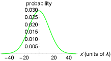
Therefore, when the atom crosses the antinode of the quantum field in the intermediate state $|b\rangle$ [Fig. 4(a)], there is no phase-shift [Fig. 4(b)] and no quadrature measurement can reveal which-path information. This is because the same phase can be obtained if the atom takes the bottom path (initial phase unaffected).

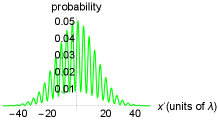
In contrast, when the atom crosses the antinode in the ground state $|c\rangle$ [Fig. 5(a)], the phase increases from $0$ to $\pi$ [Fig. 5(b)]. In that case, the internal atomic state does not reveal path-information by itself. However, the path-information is stored in the phase of the quantum field and can be extracted through a $X$ quadrature measurement.

In general, if the quadrature

is measured with an eigenvalue $\chi_{\theta}$, the corresponding eigenstate $|\chi_{\theta}\rangle$ is an infinitely squeezed state given by Storey et al. (1993); Orszag et al. (1995)

where

with $N$ being a normalization constant. The function $H_{n}(z)$ corresponds to the Hermite polynomials with $z=(\alpha e^{-i\theta}+\alpha^{*}e^{i\theta})/2$.

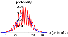
Since we consider $|g|^{2}t/\Delta=\pi$, a $X_{\theta=0}=X$ quadrature measurement with values $\chi_{\theta=0}=\pm\alpha$ determines the phase of the field and then we can know whether the atom passed through either the node or antinode (considering $\phi=0$). On other hand, if a $X_{\theta=\pi/2}=Y$ quadrature measurement is performed, and the most probable result is obtained ($\chi_{\theta=\pi/2}=0$), no path-information is obtained and interference appears on the screen, since that from the most probable result no path information is inferred (Fig. 6).

In a typical double-slit scheme we can configure several cases in order to study the quantum duality between distinguishabilily (particle-like) and visibility (wave-like) Englert (1996). Now, if a correlation is established between some intrinsical property of a particle and the possible paths, the wave-particle duality can be modified depending on the degree of entanglement in the system. Recently, it has been experimentally proven the relation among distinguishabilily ($D_{0}$), visibility ($V_{0}$) and concurrence ($C_{0}$) Qian et al. (2020) which can be written as

with

Greenberger and Yasin (1988); Jaeger et al. (1995, 1993); Wootters and Zurek (1979) where $c_{\uparrow}$ and $c_{\downarrow}$ are coefficients that define the probabilities for the atom of taking the top or bottom path, while $\gamma\equiv\langle\Phi_{\uparrow}|\Phi_{\downarrow}\rangle$, where the normalized states $|\Phi_{\uparrow,\downarrow}\rangle$ correspond to intrinsic degrees of freedom of the particle, in our case the internal atomic state.

Cases of special interest are shown on the surface of the sphere in the Fig. 7. The point $C_{0}=1$, with coefficients $c_{\uparrow}=c_{\downarrow}=1/\sqrt{2}$ and $\gamma=0$, represents a special scenario in which, based on the definitions of $D_{0}$ and $V_{0}$, visibility and distinguishability are equal to zero. So, what would we expect to observe on the screen after the double slit?

In the next section we analyze different cases considering our scheme, in which the which-path information can be stored in the phase-shift of the quantum field, but also it can be controlled through the coefficients $c_{\uparrow}$ and $c_{\downarrow}$, and we show the different patterns that are obtained in each case shown on the sphere. Finally, we show how the classic field can change the initial visibility and which-path information as $\varepsilon$ increases from $0$ to higher values and how the corresponding patterns are modified.

This is the simpler stage. Distinguishability, visibility and concurrence depend only on the choice of the coefficients of reflection $c_{\uparrow}$, transmission $c_{\downarrow}$ and $\gamma$. For instance, in the case $V_{0}=1$ the internal atomic state is $|c\rangle$ in both paths, thus $\phi=0$ and $\gamma=\cos\phi=1$, which ensures $C_{0}=0$. Furthermore, the coefficients $c_{\uparrow}$ and $c_{\downarrow}$ are taken to be same, then $D_{0}=0$. Therefore, this corresponds to a case of total interference that is shown in green in the Fig. 8(a). The values $c_{\uparrow}=1$, $c_{\downarrow}=0$ and $0\leq\gamma\leq 1$ correspond to other case, $D_{0}=1$, which does not show fringes of visibility [Fig. 8(c)]. Perhaps the most interesting case is $C_{0}=1$ [Fig. 8(e)], in which there is no distinguishability nor visibility. In this case, the observed pattern on the screen is similar to the typical diffraction pattern of the case $D_{0}=1$. The rest of distributions represent intermediate cases which can be obtained considering the appropriate coefficients.

Here we consider the quantum field with an amplitude $\alpha=\sqrt{8}$, located immediately after the double-slit (see Fig. 1). As stated earlier in the Section II.C, the quantum field can store path-information in case the atom crosses the antinode in the internal state $|c\rangle$. Otherwise (state $|b\rangle$ in the upper path, or state $|c\rangle$ lower path), the phase of the quantum field remains unaffected. Thus, we have three sources of path-information: i) the choice of the coefficients $c_{\uparrow}$ and $c_{\downarrow}$, ii) the possible phase-shift of the quantum field, and iii) the internal atomic state of the atom after double-slit.
$\bullet$ i) As in the stage 1, if $c_{\uparrow}=1$ and $c_{\downarrow}=0$, we immediately get path information.
$\bullet$ ii) If we choose $c_{\uparrow}=c_{\downarrow}$ and $\phi=0$ ($\gamma=1$), the internal atomic state in both paths is $|c\rangle$ and the path-information is recorded in the phase of the field, and can be extracted by measuring the $X$ quadrature.
$\bullet$ iii) Finally, for $c_{\uparrow}=c_{\downarrow}$ and $\phi=\pi/2$ ($\gamma=0$), the top and bottom paths are correlated to the atomic states $|b\rangle$ and $|c\rangle$, respectively. In that case the field does not store path-information. However, path-information related to the atomic states is stored and can be obtained by measuring the internal atomic state once the atom leaves the cavity.

Therefore, in presence of the quantum field we will not observe fringes of interference in any of the cases on the sphere [see blue lines in the Fig. 9(a) - 9(g)], because each case corresponds either, to one of the situations i), ii), iii), or to some intermediate state. In fact, i), ii) and iii) correspond to the cases in which the coefficients $c_{\uparrow,\downarrow}$ and $\gamma$ satisfy $D_{0}=1$, $V_{0}=1$ and $C_{0}=1$, respectively. Nevertheless, fringe visibility can be restored if the path-information is erased. In order to achieve that, the first option is reducing the amplitude of the quantum field, so that the $X$ quadrature measurement becomes ambiguous and does not reveal path-information. In this way the interference is partially restored [red lines in Fig. 9(a), 9(b), 9(f), 9(g)]. In other cases, like $D_{0}=1$ [Fig. 9(c)], $D_{0}=C_{0}$ [Fig. 9(d)] and $C_{0}=1$ [Fig. 9(e)], interference cannot be restored.

A second option is performing a $Y$ quadrature measurement of the field. In this case the path-information is completely erased and interference is restored, since we assume the outcome of our measurement as the most probable result that corresponds to $\chi_{\theta=\pi/2}=0$. The green lines in the Fig. 8(a) - 8(g) are the distributions we would expect to see on the screen if a $Y$ quadrature measurement is performed on the quantum field. This is the same result that we would obtain if the quantum field were not present.

Finally, we consider the double-slit scheme with both quantum and classic fields. When the classical light is present, it affects the final phase of the quantum field after the interaction, because the terms whose phases depend on $\varepsilon$ appear in the evolution operator. As a consequence, interference and path-information are altered. As in the previous stage, the phase-shift produced by $\varepsilon$ also depends on the internal atomic state $|c\rangle$ or $|b\rangle$ present in the top path.

$\bullet$ The top path and internal state $|b\rangle$: When $\varepsilon=0$, we have already seen that the phase of the quantum field does not change and thus we cannot obtain which-path information. However, for different values of $\varepsilon$, the phase of the quantum field moves away from its initial value and then we are able to get distinguishability (Fig. 10). Therefore, the higher the value of $\varepsilon$ the more path-information we get, at the expense of visibility.

$\bullet$ The top path and internal state $|c\rangle$: In this case, starting from $\varepsilon=0$, as we increase the classical field, the $X$ quadrature measurement becomes ambiguous, decreasing the which-path information and therefore increasing the visibility(Fig. 11).

To show the effect of the classic field on the atomic distributions, we analyse the same cases shown before, considering $\varepsilon=3$ and $\alpha=\sqrt{8}$. In the Fig. 12 we can see how the visibility fringes are restored (red lines). Thus, there is less available path-information with respect to the stage 2 (blue lines). If we look again the case $V_{0}=1$ [Fig. 12(a)], we see now partial interference because now there is a probability of measuring a phase $\eta=0$ and get visibility, or $\eta=\pi$ and gain path-information. Cases like $V_{0}=D_{0}$ [Fig. 12(b)], $C_{0}=V_{0}$ [Fig. 12(f)] and $D_{0}=C_{0}=V_{0}$ [Fig. 12(g)] also show how the interference can be restored. On other hand, in the cases $D_{0}=1$ [Fig. 12(c)], $D_{0}=C_{0}$ [Fig. 12(d)] and $C_{0}=1$ [Fig. 12(e)] there is no interference, but these show that the atomic distributions evolve faster. This means that the initial Gaussian profiles of the atomic distribution in the position $x=0$ and $x=0.25\lambda_{CF}$ in $t^{\prime}=0$, interact with each other earlier as compared to the case $\varepsilon=0$.

References

- Bohr (1928) N. Bohr, Nature 121, 580 (1928).
- Einstein et al. (1935) A. Einstein, B. Podolsky, and N. Rosen, Phys. Rev. 47, 777 (1935).
- Wootters and Zurek (1979) W. K. Wootters and W. H. Zurek, Phys. Rev. D 19, 473 (1979).
- Aharonov and Zubairy (2005) Y. Aharonov and M. S. Zubairy, Science 307, 875 (2005).
- Scully and Zubairy (1997) M. O. Scully and M. S. Zubairy, Quantum optics (1997).
- Scully et al. (1991) M. O. Scully, B.-G. Englert, and H. Walther, Nature 351, 111 (1991).
- Storey et al. (1992) P. Storey, M. Collett, and D. Walls, Phys. Rev. Lett. 68, 472 (1992).
- Storey et al. (1993) P. Storey, M. Collett, and D. Walls, Phys. Rev. A 47, 405 (1993).
- Scully and Drühl (1982) M. O. Scully and K. Drühl, Phys. Rev. A 25, 2208 (1982).
- Englert (1996) B.-G. Englert, Phys. Rev. Lett. 77, 2154 (1996).
- Greenberger and Yasin (1988) D. M. Greenberger and A. Yasin, Physics Letters A 128, 391 (1988).
- Jaeger et al. (1995) G. Jaeger, A. Shimony, and L. Vaidman, Phys. Rev. A 51, 54 (1995).
- Jaeger et al. (1993) G. Jaeger, M. A. Horne, and A. Shimony, Phys. Rev. A 48, 1023 (1993).
- Jakob and Bergou (2010) M. Jakob and J. A. Bergou, Optics Communications 283, 827 (2010).
- Orszag and Carrasco (2020) M. Orszag and S. Carrasco, Particle states are equidistant to wave and fully-entangled states in an interferometer (2020), arXiv:2001.01375 [quant-ph] .
- Jakob and Bergou (2007) M. Jakob and J. A. Bergou, Phys. Rev. A 76, 052107 (2007).
- Wootters (1998) W. K. Wootters, Phys. Rev. Lett. 80, 2245 (1998).
- Qian et al. (2020) X.-F. Qian, K. Konthasinghe, S. K. Manikandan, D. Spiecker, A. N. Vamivakas, and J. H. Eberly, Phys. Rev. Research 2, 012016 (2020).
- Orszag et al. (1995) M. Orszag, R. Ramirez, J. C. Retamal, and C. Saavedra, Quantum and Semiclassical Optics: Journal of the European Optical Society Part B 7, 455 (1995).
- Glasgow et al. (1991) S. Glasgow, P. Meystre, M. Wilkens, and E. M. Wright, Phys. Rev. A 43, 2455 (1991).
- Gould et al. (1986) P. L. Gould, G. A. Ruff, and D. E. Pritchard, Phys. Rev. Lett. 56, 827 (1986).
- Balykin et al. (1988) V. I. Balykin, V. S. Letokhov, Y. B. Ovchinnikov, and A. I. Sidorov, Phys. Rev. Lett. 60, 2137 (1988).
- Merimeche (2006) H. Merimeche, Journal of Physics B: Atomic, Molecular and Optical Physics 39, 3723 (2006).
- Ramsey (1950) N. F. Ramsey, Phys. Rev. 78, 695 (1950).
- Hartmann et al. (2020) S. Hartmann, J. Jenewein, E. Giese, S. Abend, A. Roura, E. M. Rasel, and W. P. Schleich, Phys. Rev. A 101, 053610 (2020).
- Abend et al. (2020) S. Abend, M. Gersemann, C. Schubert, D. Schlippert, E. M. Rasel, M. Zimmermann, M. A. Efremov, A. Roura, F. A. Narducci, and W. P. Schleich, Atom interferometry and its applications (2020), arXiv:2001.10976 [physics.atom-ph] .