On the boundary of the central quadratic
hyperbolic component ¹¹12010 Mathematics Subject Classification: 37F10, 37F20

Let ${\mathcal{M}}_{d}$ denote the complex orbifold of holomorphic conjugate classes of rational maps of degree $d\geq 2$. A rational map is hyperbolic if the orbit of every critical point converges to attracting (or super-attracting) periodic cycles under iteration. Hyperbolic maps form an open subset of ${\mathcal{M}}_{d}$ and conjecturally they are dense in ${\mathcal{M}}_{d}$ [7]. A connected component of this open subset is called a hyperbolic component. Any two maps in the same hyperbolic component are quasiconformally conjugate in a neighborhood of their Julia sets [7].

The hyperbolic components of quadratic rational maps have been intensively studied and fruitful results have been obtained. For example, Rees [9] gave a classification of the hyperbolic components (see also [5]), and proved the boundedness of certain one real dimension loci in hyperbolic components. Epstein [4] provided a boundedness result for a hyperbolic component of quadratic rational maps possessing two distinct attracting cycles. The closure of the set of quadratic rational maps having a degenerate parabolic fixed point was investigated by Buff-Écalle-Epstein in [2].

In this work, we consider the boundary of the hyperbolic component ${\mathbf{H}}$ in ${\mathcal{M}}_{2}$ containing $z\mapsto z^{2}$, which is called the central quadratic hyperbolic component. Every rational map in ${\mathbf{H}}$ has two fixed attracting (or super-attracting) points and its Julia set is a quasicircle.

Each quadratic rational map has exactly three fixed points (counting the multiplicity). Let $\lambda_{1},\lambda_{2},\lambda_{3}$ be the eigenvalues at fixed points. These three eigenvalues determine the quadratic rational map up to holomorphic conjugacy ([5, Lemma 3.1]). If the three fixed points are distinct, then by the Rational Fixed Point Theorem ([6, Theorem 12.4]), we have

If a quadratic rational map has at least two distinct fixed points, conjugating the map by a Möbius transformation if necessary, we may assume that $0$ and $\infty$ are the two fixed points and the eigenvalues at them are $\lambda_{1}$ and $\lambda_{2}$ respectively. Thus the holomorphic conjugacy class of the map can be represented by

with $\lambda_{1}\lambda_{2}\neq 1$. Note that $f_{\lambda_{1},\lambda_{2}}$ is holomorphically conjugated to $f_{\lambda_{2},\lambda_{1}}$. Therefore the central quadratic hyperbolic component can be expressed by

where $\mathbb{D}$ denotes the unit disk.

Recall that

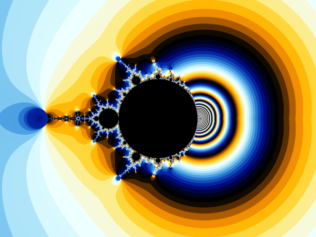
where $J(f)$ denotes the Julia set of $f$. One may refer to [1, 5, 8] for more properties about $\mathbf{M}_{1}$, see Figure 1 for a picture of ${\mathbf{M}}_{1}$ parameterized by the eigenvalue of the other fixed point.

Denote

From the definitions, we easily make the following deductions.

• (a)

  Obviously, ${\mathbf{B}}_{0}$, ${\mathbf{B}}_{1}$ and ${\mathbf{B}}_{2}$ are pairwise disjoint.

  For any $[g]\in{\mathbf{B}}_{0}\cup{\mathbf{B}}_{1}$, either $g$ has three distinct fixed points or $g$ has no repelling fixed points. Note that

  $$\overline{{\mathbf{B}}}_{2}=\{[f_{1,\lambda}]:\,\mathrm{Re}\,\lambda\geq 1\text{ but }\lambda\neq 1\}\cup\{[R]\},$$

  where $R(z)=z+1/z$. So for any $[g]\in\overline{{\mathbf{B}}}_{2}$, either $g$ has exactly two fixed points and one of them is repelling, or $g$ has a unique fixed point. Thus $({\mathbf{B}}_{0}\cup{\mathbf{B}}_{1})\cap\overline{{\mathbf{B}}}_{2}=\emptyset$.

• (b)

  It is clear that ${\mathbf{B}}_{0}\cap\mathrm{Per}_{1}(1)=\emptyset$ and ${\mathbf{B}}_{1}\cup\overline{{\mathbf{B}}}_{2}\subset\mathrm{Per}_{1}(1)$.

• (c)

  By [5, Lemma 8.2], for any $[f]\in{\mathcal{M}}_{2}$, either $J(f)$ is connected or $J(f)$ is a Cantor set. In the latter case, both critical orbits of $f$ converge to an attracting or a parabolic fixed point. If $[g]\in{\mathbf{B}}_{0}\cup{\mathbf{B}}_{1}$, then $g$ has two distinct non-repelling fixed points. Thus $J(g)$ is connected. Actually, ${\mathbf{B}}_{1}\cup\{[R]\}$ is the closure of the central component of the interior of ${\mathbf{M}}_{1}$.

Our main result is the following.

In Section 3, we exploit twist surgery to prove

which is the main part of this work.

To prove Theorem 1.1 (3), we discuss the boundedness of ${\mathbf{M}}_{1}$ in Section 4 and give a bound on ${\mathbf{M}}_{1}$ in Lemma 4.1. The bound given by Buff-Epstein is stronger than Lemma 4.1. We would like to point out that, compared to their result, Lemma 4.1 is obtained by quite simple and elementary computations. For self-containedness, we include Lemma 4.1 in this article.

Obviously, $\partial{\mathbf{H}}\cap\mathrm{Per}_{1}(1)={\mathbf{B}}_{1}\cup\overline{{\mathbf{B}}}_{2}$ by Theorem 1.1 (1).

2. One typical way to produce boundary maps of hyperbolic components is pinching. It is proved in [3] that under certain conditions, the pinching path $\{f_{t}\}$ starting from a geometrically finite rational map $f$ converges uniformly to a geometrically finite rational map $g$, and the quasiconformal conjugacy from $f$ to $f_{t}$ converges uniformly to a semi-conjugacy from $f$ to $g$. Moreover, $M[g,J]\subset\partial M[f,J]$, where $M[f,J]\subset{\mathcal{M}}_{d}$ is defined as $[h]\in M[f,J]$ if $h$ is quasiconformally conjugate to $f$ in a neighborhood of the Julia sets.

It turns out that any geometrically finite rational map $g$ with $[g]\in{\mathbf{B}}_{0}\cup{\mathbf{B}}_{1}$ is the limit of a pinching path starting from a rational map in ${\mathbf{H}}$. By Theorem 1.1 (2), if $[g]\in{\mathbf{B}}_{2}$, then $J(g)$ is disconnected. Thus it can not be obtained by pinching from ${\mathbf{H}}$.

It is obvious that ${\mathbf{H}}=M[f,J]$ for any $[f]\in{\mathbf{H}}$; and $\mathrm{Per}_{1}(1){\backslash}\mathbf{M}_{1}=M[g,J]$ for any $[g]\in\mathrm{Per}_{1}(1){\backslash}\mathbf{M}_{1}$ ([7]). By Theorem 1.1 (3), for $[g]\in{\mathbf{B}}_{2}$, $[g]\in\partial M[f,J]$ but $M[g,J]$ is not contained in $\partial M[f,J]$.

In this section, we give a direct description of the boundary $\partial{\mathbf{H}}$ by a basic discussion.

The reader may also refer to [5, Section 3] or [4, Lemma 3] for the above lemma. The statement here is slightly different from them.

In this section, we will apply twist deformation to study the dynamics of maps in ${\mathbf{B}}_{2}$.

Let $[f_{\lambda_{1},\lambda_{2}}]\in{\mathbf{H}}$ with $\lambda_{1},\lambda_{2}\neq 0$. Denote by $U$ the set of points in the Fatou set $F(f_{\lambda_{1},\lambda_{2}})$ with infinite forward orbits. Then the quotient space $U/\sim$ is a disjoint union of two tori $T_{1}$ and $T_{2}$ under the equivalence relation $z_{1}\sim z_{2}$ if $f^{n}(z_{1})=f^{m}(z_{2})$ for some integers $n,m\geq 0$. Denote by $\pi:U\to U/\sim$ the natural projection. Then each torus $T_{j}$ contains a unique point $x_{j}$ such that $\pi(c_{j})=x_{j}$, where $c_{1}$ and $c_{2}$ are the critical points of $f_{\lambda_{1},\lambda_{2}}$.

By the Koenigs Linearization Theorem ([6]), for $j=1,2$, there is a conformal map $\iota_{j}:\,\mbox{$\mathbb{C}$}/\Lambda_{j}\to T_{j}$, where $\Lambda_{j}$ is the lattice generated by $2\pi i$ and $\omega_{j}$ with $e^{\omega_{j}}=\lambda_{j}$, such that for any simple closed curve $\beta\subset\mbox{$\mathbb{C}$}/\Lambda_{j}$ corresponding to $\zeta\mapsto\zeta+2\pi i$, each component of $\pi^{-1}(\iota_{j}(\beta))$ is a Jordan curve in $U$ if $\iota_{j}(\beta)\subset T_{j}$ is disjoint from the point $x_{j}$.

For $j=1,2$, let $\gamma_{j}\subset T_{j}{\backslash}\{x_{j}\}$ be a simple closed curve such that $\iota_{j}^{-1}(\gamma_{j})$ is homotopic to the curve corresponding to $\zeta\mapsto\zeta+\omega_{j}$ in $\mbox{$\mathbb{C}$}/\Lambda_{j}$. Then each component of $\pi^{-1}(\gamma_{j})$ is an open arc. In particular, $\pi^{-1}(\gamma_{j})$ has a unique component whose endpoints contain the attracting fixed points.

Let $\tau_{j}$ be the Dehn twist along $\gamma_{j}$. We will consider the quasiconformal deformation of $f_{\lambda_{1},\lambda_{2}}$ whose projection to $T_{1}\cup T_{2}$ realizes the repeated Dehn twist $\tau_{1}^{-n}\circ\tau_{2}^{n}$. Such quasiconformal deformation can be defined as follows.

Take an annulus $A_{j}\subset T_{j}{\backslash}\{x_{j}\}$ for $j=1,2$, such that $\partial A_{j}$ consists of two disjoint simple closed curves homotopic to $\gamma_{j}$ in $T_{j}{\backslash}\{x_{j}\}$. Let $\chi_{j}$ be a conformal map from $A_{j}$ onto $\{z:\,1<|z|<r_{j}\}$. Define a quasiconformal map $\Phi_{j}$ from $\{z:\,1<|z|<r_{j}\}$ onto itself by

Now we define

For every $n\geq 1$, let $\mu_{n}$ be the Beltrami differential of $\Phi^{\circ n}$. Let $\widetilde{\mu}_{n}$ be the pullback of $\mu_{n}$ under $\pi$, i.e.,

Then there exists a quasiconformal map $\phi_{n}:\overline{\mbox{$\mathbb{C}$}}\to\overline{\mbox{$\mathbb{C}$}}$ with Beltrami differential $\widetilde{\mu}_{n}$. Set $f_{n}=\phi_{n}\circ f_{\lambda_{1},\lambda_{2}}\circ\phi_{n}^{-1}$. Then $f_{n}$ is a rational map. We call $\{[f_{n}]\}$ a twist sequence of $f_{\lambda_{1},\lambda_{2}}$ along $(\omega_{1},\omega_{2})$.

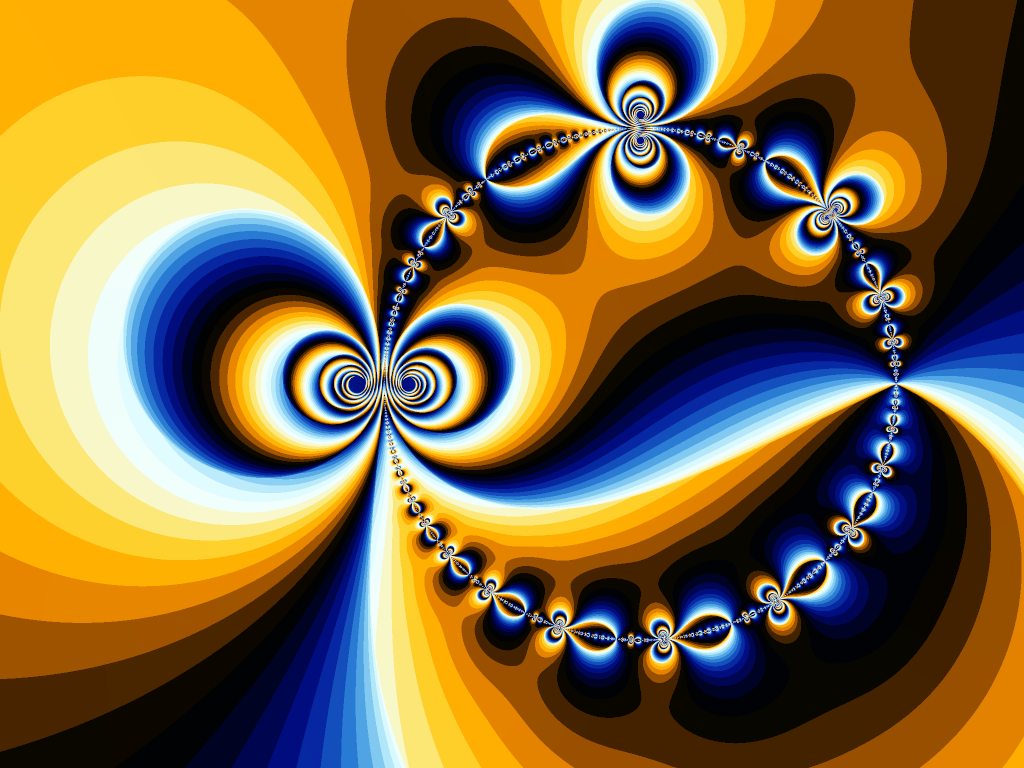
In order to illustrate the deformation of the dynamics of the twist sequence $\{f_{n}\}$ and its limit map near the Julia sets, we choose a map $[f_{\lambda_{1},\lambda_{2}}]\in{\mathbf{H}}$ such that $\lambda_{1}=\bar{\lambda}_{2}$. Then

i.e., $f_{\lambda_{1},\lambda_{2}}$ is symmetric about the unit circle and $J(f_{\lambda_{1},\lambda_{2}})$ is the unit circle.

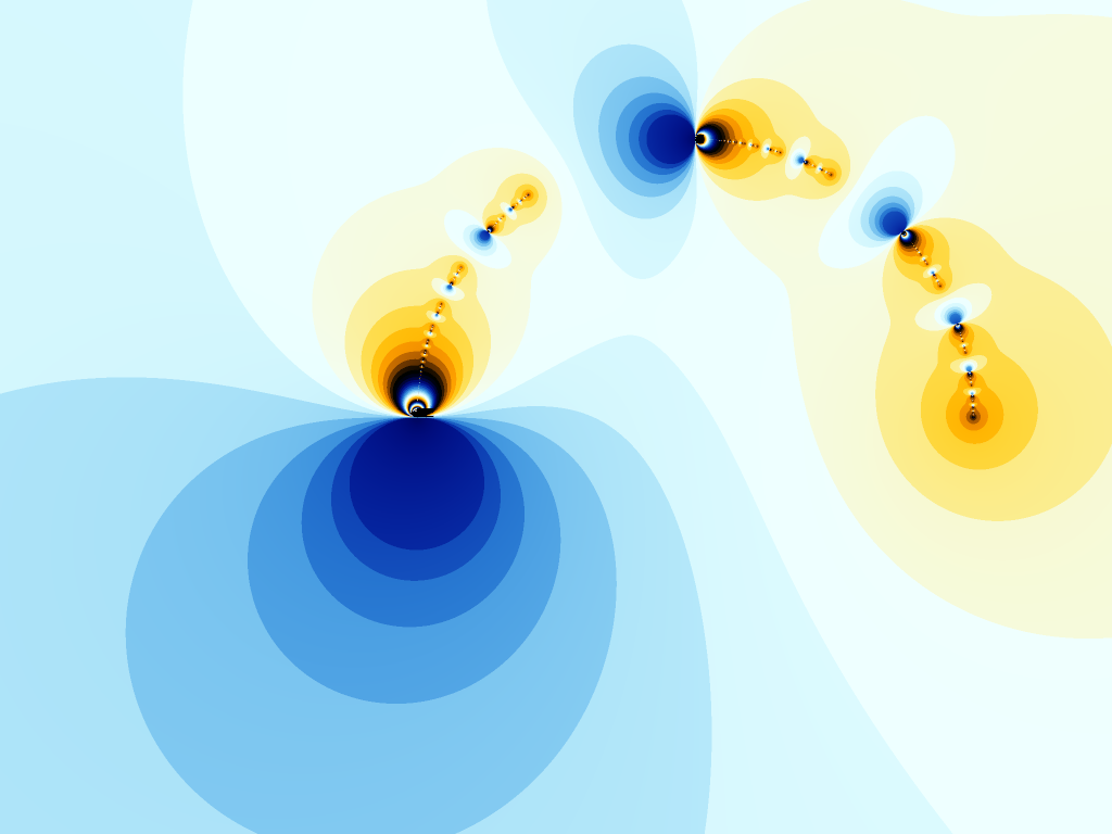
Since $\lambda_{1}=\bar{\lambda}_{2}$, we may choose $\omega_{1},\omega_{2}$ such that $e^{\omega_{1}}=\lambda_{1}$, $e^{\omega_{2}}=\lambda_{2}$ and $\omega_{1}=\bar{\omega}_{2}$. Let $\lambda_{1,n},\lambda_{2,n}$ be the eigenvalues of the attracting fixed points of the twist sequence $\{[f_{n}]\}$ of $f_{\lambda_{1},\lambda_{2}}$ along $(\omega_{1},\omega_{2})$. Then $\lambda_{1,n}=\overline{\lambda_{2,n}}$ by the definition of twist deformation. Thus $f_{\lambda_{1,n},\lambda_{2,n}}$ is also symmetric about the unit circle. By making a holomorphic conjugacy, we may choose a representative $h_{n}\in[f_{n}]$ such that $h_{n}$ is still symmetric about the unit circle, but the two attracting fixed points of $h_{n}$ are $-|\lambda_{1,n}|$ and $-1/|\lambda_{1,n}|$. Then as $n\to\infty$, $\{h_{n}\}$ uniformly converges to a quadratic rational map $h_{\infty}$. See Figure 2 for the dynamics of $h_{n}$ and Figure 3 for the dynamics of $h_{\infty}$ near Julia sets.

We may parameterize $\mathrm{Per}_{1}(1)$ by its eigenvalue at another fixed point.

References

- [1] X. Buff and A. Epstein, A parabolic Pommerenke-Levin-Yoccoz inequality, Fundamenta Mathematicae, 172 (2002), 249-289.
- [2] X. Buff, J. Écalle and A. Epstein, Limits of degenerate parabolic quadratic rational maps, Geom. Funct. Anal. 23 (2013), No. 1, 42-95.
- [3] G. Cui and L. Tan, Hyperbolic-parabolic deformations of rational maps, Sci. China: Math., 61 (2018), No. 12, 2157-2220.
- [4] A. Epstein, Bounded hyperbolic components of quadratic rational maps, Ergodic Theory Dynam. Systems, 20 (2000), No. 3, 727-748.
- [5] J. Milnor, Geometry and dynaimcs of quadratic rational maps, With an appendix by the author and Lei Tan, Experiment. Math., 2 (1993), No. 1, 37-83.
- [6] J. Milnor, Dynamics in One Complex Variable, 3rd edition, Princeton University Press, 2006.
- [7] R. Mañe, P. Sad and D. Sullivan, On the dynamics of rational maps, Ann. Sci. Éc. Norm. Sup. 16 (1983), 193-217.
- [8] C. L. Petersen and P. Roesch, The Parabolic Mandelbrot Set, arXiv:2107.09407v1.
- [9] M. Rees, Components of degree two hyperbolic rational maps, Invent. Math., 100 (1990), 357-382.
Guizhen Cui
School of Mathematical Sciences,
Shenzhen University, Shenzhen, 518052, P. R. China
and
Academy of Mathematics and Systems Science,
Chinese Academy of Sciences, Beijing, 100190, P. R. China.
[email protected]
Wenjuan Peng
Chinese Academy of Sciences, Beijing 100190, P. R. China.